Vector and Tensor
Calculus
Frankenstein’s Note
Daniel Miranda
Copyright ©2018
Permission is granted to copy, distribute and/or modify this document under the terms of the GNU Free Documentation License, Version 1.3 or any later version published by the Free Software Foundation; with no Invariant Sections, no Front-Cover Texts, and no Back-Cover Texts.
These notes were written based on and using excerpts from the book “Multivariable and Vector Calculus” by David Santos and includes excerpts from “Vector Calculus” by Michael Corral, from “Linear Algebra via Exterior Products” by Sergei Winitzki, “Linear Algebra” by David Santos and from “Introduction to Tensor Calculus” by Taha Sochi. These books are also available under the terms of the GNU Free Documentation
Li-History
These notes are based on the LATEX source of the book “Multivariable and Vector Calculus” of David Santos, which has undergone profound changes over time. In particular some examples and figures from “Vector Calculus” by Michael Corral have been added. The tensor part is based on “Linear algebra via exterior products” by Sergei Winitzki and on “Introduction to Tensor Calculus” by Taha Sochi.
What made possible the creation of these notes was the fact that these four books available are under the terms of the GNU Free Documentation License.
0.76
Corrections in chapter 8, 9 and 11.
The section 3.3 has been improved and simplified.
Third Version 0.7 - This version was released 04/2018.
Two new chapters: Multiple Integrals and Integration of Forms. Around 400 corrections in the first seven chapters. New examples. New figures.
Second Version 0.6 - This version was released 05/2017.
In this versions a lot of efforts were made to transform the notes into a more coherent text.
First Version 0.5 - This version was released 02/2017.
Acknowledgement
I would like to thank Alan Gomes, Ana Maria Slivar, Tiago Leite Dias for all they comments and cor-rections.
Contents
I. Differential Vector Calculus 1
1. Multidimensional Vectors 3
1.1. Vectors Space . . . 3
1.2. Basis and Change of Basis . . . 8
1.2.1. Linear Independence and Spanning Sets . . . 8
1.2.2. Basis . . . 10
1.2.3. Coordinates . . . 11
1.3. Linear Transformations and Matrices . . . 15
1.4. Three Dimensional Space . . . 17
1.4.1. Cross Product . . . 17
1.4.2. Cylindrical and Spherical Coordinates . . . 22
1.5. ⋆ Cross Product in the n-Dimensional Space . . . 27
1.6. Multivariable Functions . . . 28
1.6.1. Graphical Representation of Vector Fields . . . 29
1.7. Levi-Civitta and Einstein Index Notation . . . 31
1.7.1. Common Definitions in Einstein Notation . . . 35
1.7.2. Examples of Using Einstein Notation to Prove Identities . . . 36
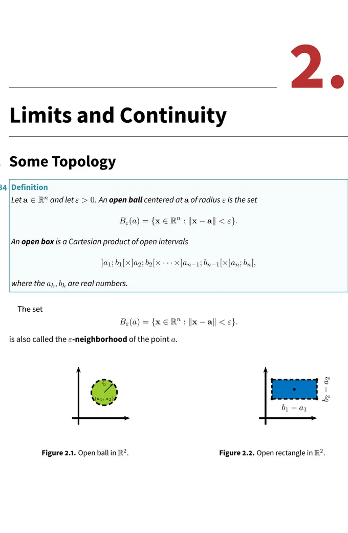
2. Limits and Continuity 39 2.1. Some Topology . . . 39
2.2. Limits . . . 44
2.3. Continuity . . . 49
2.4. ⋆ Compactness . . . . 51
3. Differentiation of Vector Function 55 3.1. Differentiation of Vector Function of a Real Variable . . . 55
3.1.1. Antiderivatives . . . 60
3.2. Kepler Law . . . 62
Contents
3.6. Properties of Differentiable Transformations . . . 72
3.7. Gradients, Curls and Directional Derivatives . . . 76
3.8. The Geometrical Meaning of Divergence and Curl . . . 83
3.8.1. Divergence . . . 83
3.8.2. Curl . . . 84
3.9. Maxwell’s Equations . . . 86
3.10. Inverse Functions . . . 87
3.11. Implicit Functions . . . 89
3.12. Common Differential Operations in Einstein Notation . . . 91
3.12.1. Common Identities in Einstein Notation . . . 92
3.12.2. Examples of Using Einstein Notation to Prove Identities . . . 94
II. Integral Vector Calculus 101 4. Multiple Integrals 103 4.1. Double Integrals . . . 103
4.2. Iterated integrals and Fubini’s theorem . . . 106
4.3. Double Integrals Over a General Region . . . 111
4.4. Triple Integrals . . . 115
4.5. Change of Variables in Multiple Integrals . . . 118
4.6. Application: Center of Mass . . . 125
4.7. Application: Probability and Expected Value . . . 128
5. Curves and Surfaces 137 5.1. Parametric Curves . . . 137
5.2. Surfaces . . . 140
5.2.1. Implicit Surface . . . 142
5.3. Classical Examples of Surfaces . . . 143
5.4. ⋆ Manifolds . . . 148
5.5. Constrained optimization. . . 149
6. Line Integrals 155 6.1. Line Integrals of Vector Fields . . . 155
6.2. Parametrization Invariance and Others Properties of Line Integrals . . . 158
6.3. Line Integral of Scalar Fields . . . 159
6.3.1. Area above a Curve . . . 160
6.4. The First Fundamental Theorem . . . 162
6.5. Test for a Gradient Field . . . 164
6.5.1. Irrotational Vector Fields . . . 164
6.5.2. Work and potential energy . . . 165
6.6. The Second Fundamental Theorem . . . 166
6.7. Constructing Potentials Functions . . . 167
Contents
6.8. Green’s Theorem in the Plane . . . 169
6.9. Application of Green’s Theorem: Area . . . 175
6.10. Vector forms of Green’s Theorem . . . 177
7. Surface Integrals 179 7.1. The Fundamental Vector Product . . . 179
7.2. The Area of a Parametrized Surface . . . 182
7.2.1. The Area of a Graph of a Function . . . 187
7.2.2. Pappus Theorem . . . 189
7.3. Surface Integrals of Scalar Functions . . . 190
7.4. Surface Integrals of Vector Functions . . . 192
7.4.1. Orientation . . . 192
7.4.2. Flux . . . 193
7.5. Kelvin-Stokes Theorem . . . 196
7.6. Gauss Theorem . . . 202
7.6.1. Gauss’s Law For Inverse-Square Fields . . . 204
7.7. Applications of Surface Integrals . . . 206
7.7.1. Conservative and Potential Forces . . . 206
7.7.2. Conservation laws . . . 207
7.8. Helmholtz Decomposition . . . 208
7.9. Green’s Identities . . . 209
III. Tensor Calculus 211 8. Curvilinear Coordinates 213 8.1. Curvilinear Coordinates . . . 213
8.2. Line and Volume Elements in Orthogonal Coordinate Systems . . . 217
8.3. Gradient in Orthogonal Curvilinear Coordinates . . . 220
8.3.1. Expressions for Unit Vectors . . . 221
8.4. Divergence in Orthogonal Curvilinear Coordinates . . . 222
8.5. Curl in Orthogonal Curvilinear Coordinates . . . 223
8.6. The Laplacian in Orthogonal Curvilinear Coordinates . . . 224
8.7. Examples of Orthogonal Coordinates . . . 225
9. Tensors 231 9.1. Linear Functional . . . 231 9.2. Dual Spaces . . . 232 9.2.1. Duas Basis . . . 233 9.3. Bilinear Forms . . . 234 9.4. Tensor . . . 235
Contents
9.5. Change of Coordinates . . . 240
9.5.1. Vectors and Covectors . . . 240
9.5.2. Bilinear Forms . . . 241
9.6. Symmetry properties of tensors . . . 241
9.7. Forms . . . 242
9.7.1. Motivation . . . 242
9.7.2. Exterior product . . . 243
9.7.3. Hodge star operator . . . 247
10. Tensors in Coordinates 249 10.1. Index notation for tensors . . . 249
10.1.1. Definition of index notation . . . 249
10.1.2. Advantages and disadvantages of index notation . . . 252
10.2. Tensor Revisited: Change of Coordinate . . . 252
10.2.1. Rank . . . 254
10.2.2. Examples of Tensors of Different Ranks . . . 255
10.3. Tensor Operations in Coordinates . . . 255
10.3.1. Addition and Subtraction . . . 256
10.3.2. Multiplication by Scalar . . . 257
10.3.3. Tensor Product . . . 257
10.3.4. Contraction . . . 258
10.3.5. Inner Product . . . 259
10.3.6. Permutation . . . 259
10.4. Kronecker and Levi-Civita Tensors . . . 260
10.4.1. Kronecker δ . . . 260
10.4.2. Permutation ϵ . . . 260
10.4.3. Useful Identities Involving δ or/and ϵ . . . 261
10.4.4. ⋆ Generalized Kronecker delta . . . 264
10.5. Types of Tensors Fields . . . 265
10.5.1. Isotropic and Anisotropic Tensors . . . 265
10.5.2. Symmetric and Anti-symmetric Tensors . . . 266
11. Tensor Calculus 269 11.1. Tensor Fields . . . 269
11.1.1. Change of Coordinates . . . 271
11.2. Derivatives . . . 273
11.3. Integrals and the Tensor Divergence Theorem . . . 276
11.4. Metric Tensor . . . 277
11.5. Covariant Differentiation . . . 278
11.6. Geodesics and The Euler-Lagrange Equations . . . 282
Contents
12. Applications of Tensor 285
12.1. The Inertia Tensor . . . 285
12.1.1. The Parallel Axis Theorem . . . 288
12.2. Ohm’s Law . . . 289
12.3. Equation of Motion for a Fluid: Navier-Stokes Equation . . . 289
12.3.1. Stress Tensor . . . 289
12.3.2. Derivation of the Navier-Stokes Equations . . . 290
13. Integration of Forms 295 13.1. Differential Forms . . . 295
13.2. Integrating Differential Forms . . . 297
13.3. Zero-Manifolds . . . 297
13.4. One-Manifolds . . . 298
13.5. Closed and Exact Forms . . . 302
13.6. Two-Manifolds . . . 306
13.7. Three-Manifolds . . . 307
13.8. Surface Integrals . . . 308
13.9. Green’s, Stokes’, and Gauss’ Theorems . . . 311
IV. Appendix 319 A. Answers and Hints 321 Answers and Hints . . . 321
B. GNU Free Documentation License 333
References 339
Part I.
1.
Multidimensional Vectors
1.1. Vectors Space
In this section we introduce an algebraic structure forRn, the vector space in n-dimensions. We assume that you are familiar with the geometric interpretation of members ofR2andR3as the rectangular coordinates of points in a plane and three-dimensional space, respectively.
AlthoughRncannot be visualized geometrically if n ≥ 4, geometric ideas from R, R2, andR3 often help us to interpret the properties ofRnfor arbitrary n.
1 Definition
The n-dimensional space,Rn, is defined as the set Rn={(x
1, x2, . . . , xn) : xk∈ R }
.
Elements v ∈ Rnwill be called vectors and will be written in boldface v. In the blackboard the vectors generally are written with an arrow ⃗v.
2 Definition
If x and y are two vectors inRntheir vector sum x + y is defined by the coordinatewise addition
x + y = (x1+ y1, x2+ y2, . . . , xn+ yn) . (1.1)
Note that the symbol “+” has two distinct meanings in (1.1): on the left, “+” stands for the newly defined addition of members ofRnand, on the right, for the usual addition of real numbers.
The vector with all components 0 is called the zero vector and is denoted by 0. It has the property that v + 0 = v for every vector v; in other words, 0 is the identity element for vector addition.
3 Definition
A real number λ∈ R will be called a scalar. If λ ∈ R and x ∈ Rnwe define scalar multiplication of a vector and a scalar by the coordinatewise multiplication
1. Multidimensional Vectors
The spaceRnwith the operations of sum and scalar multiplication defined above will be called ndimensional vector space.
The vector (−1)x is also denoted by −x and is called the negative or opposite of x We leave the proof of the following theorem to the reader.
4 Theorem
If x, z, and y are inRnand λ, λ
1and λ2are real numbers, then Ê x + z = z + x (vector addition is commutative).
Ë (x + z) + y = x + (z + y) (vector addition is associative).
Ì There is a unique vector 0, called the zero vector, such that x + 0 = x for all x in Rn. Í For each x in Rnthere is a unique vector−x such that x + (−x) = 0.
Î λ1(λ2x) = (λ1λ2)x. Ï (λ1+ λ2)x = λ1x + λ2x. Ð λ(x + z) = λx + λz. Ñ 1x = x.
Clearly, 0 = (0, 0, . . . , 0) and, if x = (x1, x2, . . . , xn), then −x = (−x1,−x2, . . . ,−xn). We write x + (−z) as x − z. The vector 0 is called the origin.
In a more general context, a nonempty set V , together with two operations +,· is said to be a
vector space if it has the properties listed in Theorem 4. The members of a vector space are called vectors.
When we wish to note that we are regarding a member ofRnas part of this algebraic structure, we will speak of it as a vector; otherwise, we will speak of it as a point.
5 Definition
The canonical ordered basis forRnis the collection of vectors {e1, e2, . . . , en}
with
ek = (0, . . . , 1, . . . , 0)
| {z }
a 1 in the k slot and 0’s everywhere else . Observe that n ∑ k=1 vkek= (v1, v2, . . . , vn) . (1.3) This means that any vector can be written as sums of scalar multiples of the standard basis. We will discuss this fact more deeply in the next section.
1.1. Vectors Space
6 Definition
Let a, b be distinct points inRnand let x = b− a ̸= 0. The parametric line passing through a in the direction of x is the set
{r ∈ Rn: r = a + tx t∈ R} .
7 Example
Find the parametric equation of the line passing through the points (1, 2, 3) and (−2, −1, 0).
Solution: ▶ The line follows the direction (
1− (−2), 2 − (−1), 3 − 0)= (3, 3, 3) . The desired equation is
(x, y, z) = (1, 2, 3) + t (3, 3, 3) . Equivalently
(x, y, z) = (−2, −1, 0) + t (3, 3, 3) . ◀
Length, Distance, and Inner Product
8 Definition
Given vectors x, y ofRn, their inner product or dot product is defined as
x•y = n ∑ k=1 xkyk. 9 Theorem
For x, y, z∈ Rn, and α and β real numbers, we have: Ê (αx + βy)•z = α(x•z) + β(y•z)
Ë x•y = y•x
Ì x•x≥ 0
Í x•x = 0 if and only if x = 0
The proof of this theorem is simple and will be left as exercise for the reader. The norm or length of a vector x, denoted as∥x∥, is defined as
1. Multidimensional Vectors
10 Definition
Given vectors x, y ofRn, their distance is
d(x, y) =∥x − y∥ =»(x− y)•(x− y) = n ∑
i=1
(xi− yi)2
If n = 1, the previous definition of length reduces to the familiar absolute value, for n = 2 and n = 3, the length and distance of Definition 10 reduce to the familiar definitions for the two and three dimensional space.
11 Definition
A vector x is called unit vector
∥x∥ = 1.
12 Definition
Let x be a non-zero vector, then the associated versor (or normalized vector) denoted ˆx is the unit
vector
ˆ
x = x
∥x∥.
We now establish one of the most useful inequalities in analysis.
13 Theorem (Cauchy-Bunyakovsky-Schwarz Inequality)
Let x and y be any two vectors inRn. Then we have |x•y| ≤ ∥x∥∥y∥.
Proof. Since the norm of any vector is non-negative, we have
∥x + ty∥ ≥ 0 ⇐⇒ (x + ty)•(x + ty)≥ 0 ⇐⇒ x•x + 2tx•y + t2y•y≥ 0 ⇐⇒ ∥x∥2+ 2tx•y + t2∥y∥2 ≥ 0.
This last expression is a quadratic polynomial in t which is always non-negative. As such its discrim-inant must be non-positive, that is,
(2x•y)2− 4(∥x∥2)(∥y∥2)≤ 0 ⇐⇒ |x•y| ≤ ∥x∥∥y∥,
giving the theorem. ■
1.1. Vectors Space The Cauchy-Bunyakovsky-Schwarz inequality can be written as
n ∑ k=1 xkyk ≤ Ñ n ∑ k=1 x2k é1/2Ñ n ∑ k=1 yk2 é1/2 , (1.4)
for real numbers xk, yk.
14 Theorem (Triangle Inequality)
Let x and y be any two vectors inRn. Then we have
∥x + y∥ ≤ ∥x∥ + ∥y∥. Proof. ||x + y||2 = (x + y)•(x + y) = x•x + 2x•y + y•y ≤ ||x||2+ 2||x||||y|| + ||y||2 = (||x|| + ||y||)2,
from where the desired result follows. ■
15 Corollary
If x, y, and z are inRn,then
|x − y| ≤ |x − z| + |z − y|.
Proof. Write
x− y = (x − z) + (z − y),
and apply Theorem 14. ■
16 Definition
Let x and y be two non-zero vectors inRn. Then the angle \(x, y)between them is given by the relation
cos \(x, y) = x•y ∥x∥∥y∥.
This expression agrees with the geometry in the case of the dot product forR2andR3.
17 Definition
Let x and y be two non-zero vectors inRn. These vectors are said orthogonal if the angle between them is 90 degrees. Equivalently, if: x•y = 0 .
1. Multidimensional Vectors
18 Definition
The hyperplane defined by the point P0and the vector n is defined as the set of points P : (x1, , x2, . . . , xn)∈ Rn, such that the vector drawn from P0to P is perpendicular to n.
Recalling that two vectors are perpendicular if and only if their dot product is zero, it follows that the desired hyperplane can be described as the set of all points P such that
n•(P− P0) = 0. Expanded this becomes
n1(x1− p1) + n2(x2− p2) +· · · + nn(xn− pn) = 0,
which is the point-normal form of the equation of a hyperplane. This is just a linear equation n1x1+ n2x2+· · · nnxn+ d = 0,
where
d =−(n1p1+ n2p2+· · · + nnpn).
1.2. Basis and Change of Basis
1.2.1. Linear Independence and Spanning Sets
19 Definition
Let λi ∈ R, 1 ≤ i ≤ n. Then the vectorial sum n ∑ j=1
λjxj
is said to be a linear combination of the vectors xi∈ Rn, 1≤ i ≤ n.
20 Definition
The vectors xi∈ Rn, 1≤ i ≤ n, are linearly dependent or tied if ∃(λ1, λ2,· · · , λn)∈ Rn\ {0} such that
n ∑
j=1
λjxj = 0,
that is, if there is a non-trivial linear combination of them adding to the zero vector.
21 Definition
The vectors xi ∈ Rn, 1≤ i ≤ n, are linearly independent or free if they are not linearly dependent.
1.2. Basis and Change of Basis That is, if λi∈ R, 1 ≤ i ≤ n then
n ∑ j=1
λjxj = 0 =⇒ λ1 = λ2 =· · · = λn= 0.
A family of vectors is linearly independent if and only if the only linear combination of them giving the zero-vector is the trivial linear combination.
22 Example
{
(1, 2, 3) , (4, 5, 6) , (7, 8, 9)} is a tied family of vectors inR3, since
(1) (1, 2, 3) + (−2) (4, 5, 6) + (1) (7, 8, 9) = (0, 0, 0) .
23 Definition
A family of vectors{x1, x2, . . . , xk, . . . ,} ⊆ Rnis said to span or generateRnif every x∈ Rncan be written as a linear combination of the xj’s.
24 Example Since n ∑ k=1 vkek= (v1, v2, . . . , vn) . (1.5) This means that the canonical basis generateRn.
25 Theorem
If{x1, x2, . . . , xk, . . . ,} ⊆ RnspansRn, then any superset {y, x1, x2, . . . , xk, . . . ,} ⊆ Rn also spansRn.
Proof. This follows at once from
l ∑ i=1 λixi = 0y + l ∑ i=1 λixi. ■ 26 Example
The family of vectors
{
i = (1, 0, 0) , j = (0, 1, 0) , k = (0, 0, 1)}
spansR3since given (a, b, c)∈ R3we may write
1. Multidimensional Vectors
27 Example
Prove that the family of vectors {
t1= (1, 0, 0) , t2= (1, 1, 0) , t3= (1, 1, 1) }
spansR3.
Solution: ▶ This follows from the identity
(a, b, c) = (a− b) (1, 0, 0) + (b − c) (1, 1, 0) + c (1, 1, 1) = (a − b)t1+ (b− c)t2+ ct3. ◀
1.2.2. Basis
28 Definition
A family E ={x1, x2, . . . , xk, . . .} ⊆ Rnis said to be a basis ofRnif Ê are linearly independent,
Ë they span Rn.
29 Example
The family
ei = (0, . . . , 0, 1, 0, . . . , 0) ,
where there is a 1 on the i-th slot and 0’s on the other n− 1 positions, is a basis for Rn.
30 Theorem
All basis ofRnhave the same number of vectors.
31 Definition
The dimension ofRnis the number of elements of any of its basis, n.
32 Theorem
Let{x1, . . . , xn} be a family of vectors in Rn. Then the x’s form a basis if and only if the n×n matrix Aformed by taking the x’s as the columns of A is invertible.
Proof. Since we have the right number of vectors, it is enough to prove that the x’s are linearly
independent. But if X = (λ1, λ2, . . . , λn), then
λ1x1+· · · + λnxn= AX.
If A is invertible, then AX = 0n =⇒ X = A−10 = 0, meaning that λ1 = λ2=· · · λn= 0, so the
x’s are linearly independent.
The reciprocal will be left as a exercise. ■
1.2. Basis and Change of Basis
33 Definition
Ê A basis E = {x1, x2, . . . , xk} of vectors in Rnis called orthogonal if
xi•xj = 0
for all i̸= j.
Ë An orthogonal basis of vectors is called orthonormal if all vectors in E are unit vectors, i.e, have norm equal to 1.
1.2.3. Coordinates
34 Theorem
Let E ={e1, e2, . . . , en} be a basis for a vector space Rn. Then any x∈ Rnhas a unique represen-tation
x = a1e1+ a2e2+· · · + anen.
Proof. Let
x = b1e1+ b2e2+· · · + bnen be another representation of x. Then
0 = (a1− b1)e1+ (a2− b2)e2+· · · + (an− bn)en.
Since{e1, e2, . . . , en} forms a basis for Rn, they are a linearly independent family. Thus we must have a1− b1= a2− b2=· · · = an− bn= 0R, that is a1= b1; a2= b2;· · · ; an= bn, proving uniqueness. ■ 35 Definition
An ordered basis E ={e1, e2, . . . , en} of a vector space Rnis a basis where the order of the xkhas been fixed. Given an ordered basis{e1, e2, . . . , en} of a vector space Rn, Theorem 34 ensures that there are unique (a1, a2, . . . , an)∈ Rnsuch that
x = a1e1+ a2e2+· · · + anen. The ak’s are called the coordinates of the vector x.
1. Multidimensional Vectors
We will denote the coordinates the vector x on the basis E by [x]E
or simply [x].
36 Example
The standard ordered basis forR3is E = {i, j, k}. The vector (1, 2, 3) ∈ R3 for example, has co-ordinates (1, 2, 3)E. If the order of the basis were changed to the ordered basis F = {i, k, j}, then (1, 2, 3)∈ R3would have coordinates (1, 3, 2)F.
Usually, when we give a coordinate representation for a vector x∈ Rn, we assume that we are using the standard basis.
37 Example
Consider the vector (1, 2, 3)∈ R3(given in standard representation). Since
(1, 2, 3) =−1 (1, 0, 0) − 1 (1, 1, 0) + 3 (1, 1, 1) ,
under the ordered basis E ={(1, 0, 0) , (1, 1, 0) , (1, 1, 1)}, (1, 2, 3) has coordinates (−1, −1, 3)E. We write
(1, 2, 3) = (−1, −1, 3)E.
38 Example
The vectors of
E ={(1, 1) , (1, 2)}
are non-parallel, and so form a basis forR2. So do the vectors
F ={(2, 1) , (1,−1)}. Find the coordinates of (3, 4)Ein the base F .
Solution: ▶ We are seeking x, y such that
3 (1, 1) + 4 (1, 2) = x 2 1 + y 1 −1 =⇒ 1 1 1 2 3 4 = 2 1 1 −1 (x, y)F . 12
1.2. Basis and Change of Basis Thus (x, y)F = 2 1 1 −1 −1 1 1 1 2 3 4 = 1 3 1 3 1 3 − 2 3 1 1 1 2 3 4 = 2 3 1 −1 3 −1 3 4 = 6 −5 F .
Let us check by expressing both vectors in the standard basis ofR2: (3, 4)E = 3 (1, 1) + 4 (1, 2) = (7, 11) , (6,−5)F = 6 (2, 1)− 5 (1, −1) = (7, 11) . ◀
In general let us consider basis E , F for the same vector spaceRn. We want to convert X
Eto YF. We let A be the matrix formed with the column vectors of E in the given order an B be the matrix formed with the column vectors of F in the given order. Both A and B are invertible matrices since the E, F are basis, in view of Theorem 32. Then we must have
AXE = BYF =⇒ YF = B−1AXE. Also,
XE = A−1BYF. This prompts the following definition.
39 Definition
Let E = {x1, x2, . . . , xn} and F = {y1, y2, . . . , yn} be two ordered basis for a vector space Rn. Let A∈ Mn×n(R) be the matrix having the x’s as its columns and let B ∈ Mn×n(R) be the matrix having the y’s as its columns. The matrix P = B−1Ais called the transition matrix from E to F and the matrix P−1= A−1Bis called the transition matrix from F to E.
40 Example
Consider the basis ofR3
E ={(1, 1, 1) , (1, 1, 0) , (1, 0, 0)}, F ={(1, 1,−1) , (1, −1, 0) , (2, 0, 0)}.
1. Multidimensional Vectors Solution: ▶ Let A = 1 1 1 1 1 0 1 0 0 , B = 1 1 2 1 −1 0 −1 0 0 .
The transition matrix from E to F is
P = B−1A = 1 1 2 1 −1 0 −1 0 0 −1 1 1 1 1 1 0 1 0 0 = 0 0 −1 0 −1 −1 1 2 1 2 1 1 1 1 1 1 0 1 0 0 = −1 0 0 −2 −1 −0 2 1 1 2 .
The transition matrix from F to E is
P−1= −1 0 0 −2 −1 0 2 1 1 2 −1 = −1 0 0 2 −1 0 0 2 2 . Now, YF = −1 0 0 −2 −1 0 2 1 1 2 1 2 3 E = −1 −4 11 2 F .
As a check, observe that in the standard basis forR3 ï 1, 2, 3 ò E = 1 ï 1, 1, 1 ò + 2 ï 1, 1, 0 ò + 3 ï 1, 0, 0 ò = ï 6, 3, 1 ò , ï −1, −4,11 2 ò F =−1 ï 1, 1,−1 ò − 4 ï 1,−1, 0 ò +11 2 ï 2, 0, 0 ò = ï 6, 3, 1 ò . ◀ 14
1.3. Linear Transformations and Matrices
1.3. Linear Transformations and Matrices
41 Definition
A linear transformation or homomorphism betweenRnandRm L : R n → Rm x 7→ L(x) , is a function which is ■ Additive: L(x + y) = L(x) + L(y), ■ Homogeneous: L(λx) = λL(x), for λ∈ R.
It is clear that the above two conditions can be summarized conveniently into L(x + λy) = L(x) + λL(y).
Assume that{xi}i∈[1;n]is an ordered basis forRn, and E ={yi}i
∈[1;m]an ordered basis forRm. Then L(x1) = a11y1+ a21y2+· · · + am1ym = a11 a21 .. . am1 E L(x2) = a12y1+ a22y2+· · · + am2ym = a12 a22 .. . am2 E .. . ... ... ... ... L(xn) = a1ny1+ a2ny2+· · · + amnym = a1n a2n .. . amn E .
1. Multidimensional Vectors 42 Definition The m× n matrix ML= a11 a12 · · · a1n a21 a22 · · · a2n
..
. ... ... ... am1 am2 · · · amn
formed by the column vectors above is called the matrix representation of the linear map L with respect to the basis{xi}i∈[1;m],{yi}i∈[1;n].
43 Example
Consider L :R3 → R3,
L (x, y, z) = (x− y − z, x + y + z, z) . Clearly L is a linear transformation.
1. Find the matrix corresponding to L under the standard ordered basis.
2. Find the matrix corresponding to L under the ordered basis (1, 0, 0) , (1, 1, 0) , (1, 0, 1) , for both the domain and the image of L.
Solution: ▶
1. The matrix will be a 3× 3 matrix. We have L (1, 0, 0) = (1, 1, 0), L (0, 1, 0) = (−1, 1, 0), and L (0, 0, 1) = (−1, 1, 1), whence the desired matrix is
1 −1 −1 1 1 1 0 0 1 .
2. Call this basis E. We have
L (1, 0, 0) = (1, 1, 0) = 0 (1, 0, 0) + 1 (1, 1, 0) + 0 (1, 0, 1) = (0, 1, 0)E, L (1, 1, 0) = (0, 2, 0) =−2 (1, 0, 0) + 2 (1, 1, 0) + 0 (1, 0, 1) = (−2, 2, 0)E, and
L (1, 0, 1) = (0, 2, 1) =−3 (1, 0, 0) + 2 (1, 1, 0) + 1 (1, 0, 1) = (−3, 2, 1)E, whence the desired matrix is
0 −2 −3 1 2 2 0 0 1 . ◀ 16
1.4. Three Dimensional Space
44 Definition
The column rank of A is the dimension of the space generated by the columns of A, while the row rank of A is the dimension of the space generated by the rows of A.
A fundamental result in linear algebra is that the column rank and the row rank are always equal. This number (i.e., the number of linearly independent rows or columns) is simply called the rank of A.
1.4. Three Dimensional Space
In this section we particularize some definitions to the important case of three dimensional space
45 Definition
The 3-dimensional space is defined and denoted by
R3 ={r = (x, y, z) : x∈ R, y ∈ R, z ∈ R}.
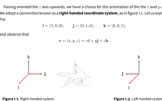
Having oriented the z axis upwards, we have a choice for the orientation of the the x and y-axis. We adopt a convention known as a right-handed coordinate system, as in figure 1.1. Let us explain. Put
i = (1, 0, 0), j = (0, 1, 0), k = (0, 0, 1),
and observe that
r = (x, y, z) = xi + yj + zk.
j k
i
j
Figure 1.1. Right-handed system.
Figure 1.2. Right Hand.
j
k
i j
Figure 1.3. Left-handed system.
1.4.1. Cross Product
The cross product of two vectors is defined only in three-dimensional spaceR3. We will define a generalization of the cross product for the n dimensional space in the section 1.5.
1. Multidimensional Vectors
46 Definition
Let x, y, z be vectors inR3, and let λ∈ R be a scalar. The cross product × is a closed binary opera-tion satisfying
Ê Anti-commutativity: x × y = −(y × x) Ë Bilinearity:
(x + z)× y = x × y + z × y and x × (z + y) = x × z + x × y Ì Scalar homogeneity: (λx) × y = x × (λy) = λ(x × y)
Í x × x = 0 Î Right-hand Rule:
i× j = k, j × k = i, k × i = j.
It follows that the cross product is an operation that, given two non-parallel vectors on a plane, allows us to “get out” of that plane.
47 Example Find (1, 0,−3) × (0, 1, 2) . Solution: ▶ We have (i− 3k) × (j + 2k) = i × j + 2i × k − 3k × j − 6k × k = k− 2j + 3i + 0 = 3i− 2j + k Hence (1, 0,−3) × (0, 1, 2) = (3, −2, 1) . ◀
The cross product of vectors inR3is not associative, since
i× (i × j) = i × k = −j
but
(i× i) × j = 0 × j = 0. Operating as in example 47 we obtain
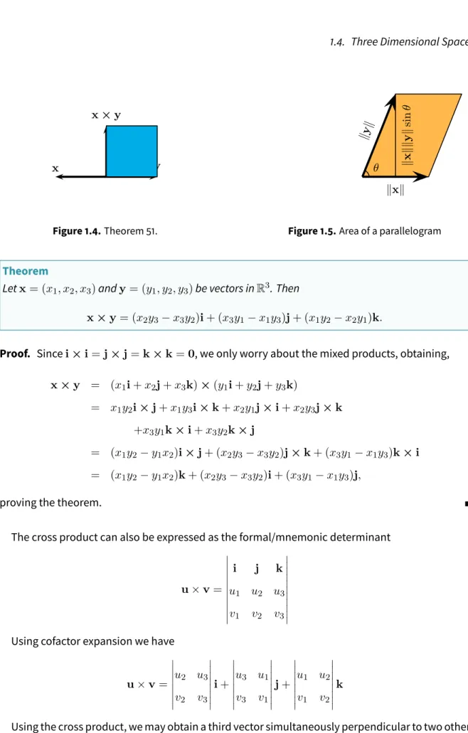
1.4. Three Dimensional Space x× y y x Figure 1.4. Theorem 51. ∥x∥ ∥y∥ θ ∥ x∥∥ y∥ sin θ
Figure 1.5. Area of a parallelogram
48 Theorem
Let x = (x1, x2, x3)and y = (y1, y2, y3)be vectors inR3. Then
x× y = (x2y3− x3y2)i + (x3y1− x1y3)j + (x1y2− x2y1)k.
Proof. Since i× i = j × j = k × k = 0, we only worry about the mixed products, obtaining, x× y = (x1i + x2j + x3k)× (y1i + y2j + y3k)
= x1y2i× j + x1y3i× k + x2y1j× i + x2y3j× k
+x3y1k× i + x3y2k× j
= (x1y2− y1x2)i× j + (x2y3− x3y2)j× k + (x3y1− x1y3)k× i = (x1y2− y1x2)k + (x2y3− x3y2)i + (x3y1− x1y3)j,
proving the theorem. ■
The cross product can also be expressed as the formal/mnemonic determinant
u× v = i j k u1 u2 u3 v1 v2 v3
Using cofactor expansion we have
u× v = u2 u3 v2 v3 i + u3 u1 v3 v1 j + u1 u2 v1 v2 k
Using the cross product, we may obtain a third vector simultaneously perpendicular to two other vectors in space.
1. Multidimensional Vectors
49 Theorem
x⊥ (x × y) and y ⊥ (x × y), that is, the cross product of two vectors is simultaneously
perpen-dicular to both original vectors.
Proof. We will only check the first assertion, the second verification is analogous. x•(x× y) = (x1i + x2j + x3k)•((x2y3− x3y2)i
+(x3y1− x1y3)j + (x1y2− x2y1)k)
= x1x2y3− x1x3y2+ x2x3y1− x2x1y3+ x3x1y2− x3x2y1 = 0,
completing the proof. ■
Although the cross product is not associative, we have, however, the following theorem.
50 Theorem a× (b × c) = (a•c)b− (a•b)c. Proof. a× (b × c) = (a1i + a2j + a3k)× ((b2c3− b3c2)i+ +(b3c1− b1c3)j + (b1c2− b2c1)k) = a1(b3c1− b1c3)k− a1(b1c2− b2c1)j− a2(b2c3− b3c2)k +a2(b1c2− b2c1)i + a3(b2c3− b3c2)j− a3(b3c1− b1c3)i = (a1c1+ a2c2+ a3c3)(b1i + b2j + b3i)+
(−a1b1− a2b2− a3b3)(c1i + c2j + c3i) = (a•c)b− (a•b)c,
completing the proof. ■
51 Theorem
Let \(x, y)∈ [0; π] be the convex angle between two vectors x and y. Then ||x × y|| = ||x||||y|| sin \(x, y).
1.4. Three Dimensional Space x z a × b y b b b b θ Figure 1.6. Theorem 497. x y z b M M b A b B b C b D b A′ b B′ bN b C′ b D′ b P Figure 1.7. Example ??. Proof. We have
||x × y||2 = (x2y3− x3y2)2+ (x3y1− x1y3)2+ (x1y2− x2y1)2 = x22y23− 2x2y3x3y2+ x23y22+ x23y12− 2x3y1x1y3+
+x21y32+ x21y22− 2x1y2x2y1+ x22y21
= (x21+ x22+ x23)(y21+ y22+ y32)− (x1y1+ x2y2+ x3y3)2 = ||x||2||y||2− (x•y)2
= ||x||2||y||2− ||x||2||y||2cos2(x, y)\ = ||x||2||y||2sin2(x, y),\
whence the theorem follows. ■
Theorem 51 has the following geometric significance: ∥x × y∥ is the area of the parallelogram formed when the tails of the vectors are joined. See figure 1.5.
The following corollaries easily follow from Theorem 51.
52 Corollary
Two non-zero vectors x, y satisfy x× y = 0 if and only if they are parallel.
53 Corollary (Lagrange’s Identity)
||x × y||2=∥x∥2∥y∥2− (x•y)2. The following result mixes the dot and the cross product.
54 Theorem
Let x, y, z, be linearly independent vectors inR3. The signed volume of the parallelepiped spanned by them is (x× y) • z.
Proof. See figure 1.6. The area of the base of the parallelepiped is the area of the parallelogram
determined by the vectors x and y, which has area∥x × y∥. The altitude of the parallelepiped is ∥z∥ cos θ where θ is the angle between z and x × y. The volume of the parallelepiped is thus
1. Multidimensional Vectors
Since we may have used any of the faces of the parallelepiped, it follows that (x× y)•z = (y× z)•x = (z× x)•y.
In particular, it is possible to “exchange” the cross and dot products:
x•(y× z) = (x × y)•z
1.4.2. Cylindrical and Spherical Coordinates
λ3e3 b O b P v e1 e3 e2 b K λ1e1 λ2e2 −−→ OK
Let B ={x1, x2, x3} be an ordered basis for R3. As we have al-ready seen, for every v∈ Rnthere is a unique linear combination of the basis vectors that equals v:
v = xx1+ yx2+ zx3.
The coordinate vector of v relative to E is the sequence of coordinates [v]E = (x, y, z).
In this representation, the coordinates of a point (x, y, z) are determined by following straight paths starting from the origin: first parallel to x1, then parallel to the x2, then parallel to the x3, as in Figure 1.7.1.
In curvilinear coordinate systems, these paths can be curved. We will provide the definition of curvilinear coordinate systems in the section 3.10 and 8. In this section we provide some examples: the three types of curvilinear coordinates which we will consider in this section are polar coordi-nates in the plane cylindrical and spherical coordicoordi-nates in the space.
Instead of referencing a point in terms of sides of a rectangular parallelepiped, as with Cartesian coordinates, we will think of the point as lying on a cylinder or sphere. Cylindrical coordinates are often used when there is symmetry around the z-axis; spherical coordinates are useful when there is symmetry about the origin.
Let P = (x, y, z) be a point in Cartesian coordinates inR3, and let P
0= (x, y, 0)be the projection
of P upon the xy-plane. Treating (x, y) as a point inR2, let (r, θ) be its polar coordinates (see Figure 1.7.2). Let ρ be the length of the line segment from the origin to P , and let ϕ be the angle between that line segment and the positive z-axis (see Figure 1.7.3). ϕ is called the zenith angle. Then the
cylindrical coordinates (r, θ, z) and the spherical coordinates (ρ, θ, ϕ) of P (x, y, z) are defined
as follows:1
1This “standard” definition of spherical coordinates used by mathematicians results in a left-handed system. For this
reason, physicists usually switch the definitions of θ and ϕ to make (ρ, θ, ϕ) a right-handed system.
1.4. Three Dimensional Space x y z 0 P(x, y, z) P0(x, y, 0) θ x y z r Figure 1.8. Cylindrical coordinates Cylindrical coordinates (r, θ, z): x = r cos θ r = » x2+ y2 y = r sin θ θ = tan−1 Åy x ã z = z z = z where 0≤ θ ≤ π if y ≥ 0 and π < θ < 2π if y < 0 x y z 0 P(x, y, z) P0(x, y, 0) θ x y z ρ ϕ Figure 1.9. Spherical coordinates Spherical coordinates (ρ, θ, ϕ): x = ρ sin ϕ cos θ ρ =»x2+ y2+ z2 y = ρ sin ϕ sin θ θ = tan−1
Å y x ã z = ρ cos ϕ ϕ = cos−1 Ç z √ x2+ y2+ z2 å where 0≤ θ ≤ π if y ≥ 0 and π < θ < 2π if y < 0
Both θ and ϕ are measured in radians. Note that r ≥ 0, 0 ≤ θ < 2π, ρ ≥ 0 and 0 ≤ ϕ ≤ π. Also, θis undefined when (x, y) = (0, 0), and ϕ is undefined when (x, y, z) = (0, 0, 0).
55 Example
Convert the point (−2, −2, 1) from Cartesian coordinates to (a) cylindrical and (b) spherical coordi-nates.
Solution: ▶ (a) r = »(−2)2+ (−2)2 = 2√2, θ = tan−1 Ç −2 −2 å = tan−1(1) = 5π 4 , since y =−2 < 0. ∴ (r, θ, z) = Ç 2√2,5π 4 , 1 å (b) ρ =»(−2)2+ (−2)2+ 12 =√9 = 3, ϕ = cos−1 Ç 1 3 å ≈ 1.23 radians. ∴ (ρ, θ, ϕ) = Ç 3,5π 4 , 1.23 å ◀
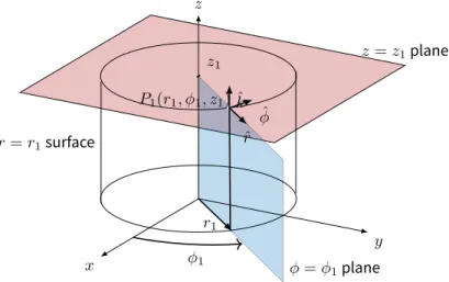
For cylindrical coordinates (r, θ, z), and constants r0, θ0and z0, we see from Figure 8.3 that the
surface r = r0is a cylinder of radius r0centered along the z-axis, the surface θ = θ0is a half-plane
1. Multidimensional Vectors y z x 0 r0 (a) r = r0 y z x 0 θ0 (b) θ = θ0 y z x 0 z0 (c) z = z0 Figure 1.10. Cylindrical coordinate surfaces
unit vectors ˆr, ˆθvary from point to point, unlike the corresponding Cartesian unit vectors.
x y z r = r1surface z = z1plane ϕ = ϕ1plane P1(r1, ϕ1, z1) ˆ r ˆ ϕ ˆ k ϕ1 r1 z1
For spherical coordinates (ρ, θ, ϕ), and constants ρ0, θ0and ϕ0, we see from Figure 1.11 that the
surface ρ = ρ0is a sphere of radius ρ0centered at the origin, the surface θ = θ0 is a half-plane
emanating from the z-axis, and the surface ϕ = ϕ0is a circular cone whose vertex is at the origin.
y z x 0 ρ0 (a) ρ = ρ0 y z x 0 θ0 (b) θ = θ0 y z x 0 ϕ0 (c) ϕ = ϕ0 Figure 1.11. Spherical coordinate surfaces
Figures 8.3(a) and 1.11(a) show how these coordinate systems got their names.
Sometimes the equation of a surface in Cartesian coordinates can be transformed into a simpler equation in some other coordinate system, as in the following example.
1.4. Three Dimensional Space
56 Example
Write the equation of the cylinder x2+ y2= 4in cylindrical coordinates.
Solution: ▶ Since r =√x2+ y2, then the equation in cylindrical coordinates is r = 2.◀ Using spherical coordinates to write the equation of a sphere does not necessarily make the equation simpler, if the sphere is not centered at the origin.
57 Example
Write the equation (x− 2)2+ (y− 1)2+ z2 = 9in spherical coordinates.
Solution: ▶ Multiplying the equation out gives
x2+ y2+ z2− 4x − 2y + 5 = 9 , so we get ρ2− 4ρ sin ϕ cos θ − 2ρ sin ϕ sin θ − 4 = 0 , or
ρ2− 2 sin ϕ (2 cos θ − sin θ ) ρ − 4 = 0
after combining terms. Note that this actually makes it more difficult to figure out what the surface is, as opposed to the Cartesian equation where you could immediately identify the surface as a sphere of radius 3 centered at (2, 1, 0).◀
58 Example
Describe the surface given by θ = z in cylindrical coordinates.
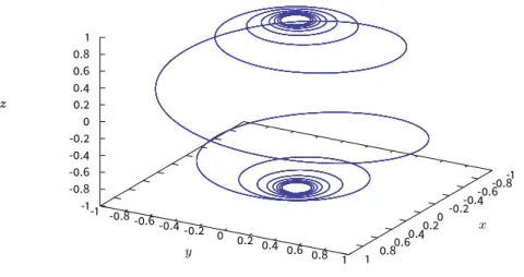
Solution: ▶ This surface is called a helicoid. As the (vertical) z coordinate increases, so does the
angle θ, while the radius r is unrestricted. So this sweeps out a (ruled!) surface shaped like a spiral staircase, where the spiral has an infinite radius. Figure 1.12 shows a section of this surface restricted to 0≤ z ≤ 4π and 0 ≤ r ≤ 2. ◀
1. Multidimensional Vectors
Exercises
A
For Exercises 1-4, find the (a) cylindrical and (b) spherical coordinates of the point whose Cartesian coordinates are given.
1. (2, 2√3,−1) 2. (−5, 5, 6)
3. (√21,−√7, 0) 4. (0,√2, 2)
For Exercises 5-7, write the given equation in (a) cylindrical and (b) spherical coordinates. 5. x2+ y2+ z2 = 25
6. x2+ y2= 2y
7. x2+ y2+ 9z2 = 36
B
8. Describe the intersection of the surfaces whose equations in spherical coordinates are θ = π 2 and ϕ = π
4.
9. Show that for a ̸= 0, the equation ρ = 2a sin ϕ cos θ in spherical coordinates describes a sphere centered at (a, 0, 0) with radius|a|.
C
10. Let P = (a, θ, ϕ) be a point in spherical coordinates, with a > 0 and 0 < ϕ < π. Then P lies on the sphere ρ = a. Since 0 < ϕ < π, the line segment from the origin to P can be extended to intersect the cylinder given by r = a (in cylindrical coordinates). Find the cylindrical coordinates of that point of intersection.
11. Let P1and P2be points whose spherical coordinates are (ρ1, θ1, ϕ1)and (ρ2, θ2, ϕ2),
respec-tively. Let v1be the vector from the origin to P1, and let v2be the vector from the origin to P2.
For the angle γ between
cos γ = cos ϕ1 cos ϕ2+ sin ϕ1 sin ϕ2 cos( θ2− θ1).
This formula is used in electrodynamics to prove the addition theorem for spherical harmon-ics, which provides a general expression for the electrostatic potential at a point due to a unit charge. See pp. 100-102 in [36].
12. Show that the distance d between the points P1and P2with cylindrical coordinates (r1, θ1, z1)
and (r2, θ2, z2), respectively, is
d =»r2
1 + r22− 2r1r2cos( θ2− θ1) + (z2− z1)2.
13. Show that the distance d between the points P1and P2with spherical coordinates (ρ1, θ1, ϕ1)
and (ρ2, θ2, ϕ2), respectively, is
d =»ρ2
1+ ρ22 − 2ρ1ρ2[sin ϕ1 sin ϕ2 cos( θ2− θ1) + cos ϕ1 cos ϕ2] .
1.5. ⋆ Cross Product in the n-Dimensional Space
1.5. ⋆ Cross Product in the n-Dimensional Space
In this section we will answer the following question: Can one define a cross product in the n-dimensional space so that it will have properties similar to the usual 3 n-dimensional one?
Clearly the answer depends which properties we require.
The most direct generalizations of the cross product are to define either:
■ a binary product× : Rn× Rn→ Rnwhich takes as input two vectors and gives as output a vector;
■ a n− 1-ary product × : R|n× · · · × R{z n} n−1 times
→ Rnwhich takes as input n− 1 vectors, and gives as output one vector.
Under the correct assumptions it can be proved that a binary product exists only in the dimen-sions 3 and 7. A simple proof of this fact can be found in [51].
In this section we focus in the definition of the n− 1-ary product.
59 Definition
Let v1, . . . , vn−1be vectors in Rn,, and let λ∈ R be a scalar. Then we define their generalized cross product vn= v1× · · · × vn−1as the (n− 1)-ary product satisfying
Ê Anti-commutativity: v1× · · · vi× vi+1× · · · × vn−1=−v1× · · · vi+1× vi× · · · × vn−1, i.e, changing two consecutive vectors a minus sign appears.
Ë Bilinearity: v1× · · · vi+ x× vi+1× · · · × vn−1= v1× · · · vi× vi+1× · · · × vn−1+ v1× · · · x × vi+1× · · · × vn−1
Ì Scalar homogeneity: v1× · · · λvi× vi+1× · · · × vn−1= λv1× · · · vi× vi+1× · · · × vn−1 Í Right-hand Rule: e1×· · ·×en−1= en, e2×· · ·×en= e1,and so forth for cyclic permutations
of indices.
We will also write
×
(v1, . . . , vn−1) := v1× · · · vi× vi+1× · · · × vn−1In coordinates, one can give a formula for this (n− 1)-ary analogue of the cross product in Rn by:
1. Multidimensional Vectors
60 Proposition
Let e1, . . . , enbe the canonical basis of Rnand let v1, . . . , vn−1be vectors in Rn,with coordinates:
v1 = (v11, . . . v1n) (1.6) .. . (1.7) vi = (vi1, . . . vin) (1.8) .. . (1.9) vn= (vn1, . . . vnn) (1.10)
in the canonical basis. Then
×
(v1, . . . , vn−1) = v11 · · · v1n .. . . .. ... vn−11 · · · vn−1n e1 · · · en .This formula is very similar to the determinant formula for the normal cross product inR3except that the row of basis vectors is the last row in the determinant rather than the first.
The reason for this is to ensure that the ordered vectors (v1, ..., vn−1,
×
(v1, ..., vn−1)) have a positive orientation with respect to(e1, ..., en).
61 Proposition
The vector product have the following properties: The vector
×
(v1, . . . , vn−1)is perpendicular to vi, ÊË the magnitude of
×
(v1, . . . , vn−1)is the volume of the solid defined by the vectors v1, . . . vi−1Ì vn•v1× · · · × vn−1= v11 · · · v1n .. . . .. ... vn−11 · · · vn−1n vn1 · · · vnn .
1.6. Multivariable Functions
Let A⊆ Rn. For most of this course, our concern will be functions of the form f : A⊆ Rn→ Rm.
1.6. Multivariable Functions If m = 1, we say that f is a scalar field. If m≥ 2, we say that f is a vector field.
We would like to develop a calculus analogous to the situation inR. In particular, we would like to examine limits, continuity, differentiability, and integrability of multivariable functions. Needless to say, the introduction of more variables greatly complicates the analysis. For example, recall that the graph of a function f : A→ Rm, A⊆ Rn. is the set
{(x, f(x)) : x ∈ A)} ⊆ Rn+m.
If m + n > 3, we have an object of more than three-dimensions! In the case n = 2, m = 1, we have a tri-dimensional surface. We will now briefly examine this case.
62 Definition
Let A ⊆ R2and let f : A → R be a function. Given c ∈ R, the level curve at z = c is the curve resulting from the intersection of the surface z = f (x, y) and the plane z = c, if there is such a curve.
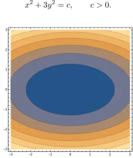
63 Example
The level curves of the surface f (x, y) = x2+ 3y2(an elliptic paraboloid) are the concentric ellipses x2+ 3y2 = c, c > 0. -3 -2 -1 0 1 2 3 -3 -2 -1 0 1 2 3
Figure 1.13. Level curves for f (x, y) = x2+ 3y2.
1.6.1. Graphical Representation of Vector Fields
In this section we present a graphical representation of vector fields. For this intent, we limit our-selves to low dimensional spaces.
A vector field v : R3 → R3is an assignment of a vector v = v(x, y, z) to each point (x, y, z) of a subset U ⊂ R3. Each vector v of the field can be regarded as a ”bound vector” attached to the corresponding point (x, y, z). In components
1. Multidimensional Vectors
64 Example
Sketch each of the following vector fields.
F = xi + yj F =−yi + xj r = xi + yj + zk
Solution: ▶
a) The vector field is null at the origin; at other points, F is a vector pointing away from the origin; b) This vector field is perpendicular to the first one at every point;
c) The vector field is null at the origin; at other points, F is a vector pointing away from the origin. This is the 3-dimensional analogous of the first one.◀
-3 -2 -1 0 1 2 3 -3 -2 -1 0 1 2 3 -3 -2 -1 0 1 2 3 -3 -2 -1 0 1 2 3 −1 −0.5 0 0.5 1 −1 0 1 −1 0 1 65 Example
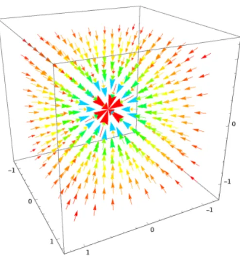
Suppose that an object of mass M is located at the origin of a three-dimensional coordinate system. We can think of this object as inducing a force field g in space. The effect of this gravitational field is to attract any object placed in the vicinity of the origin toward it with a force that is governed by Newton’s Law of Gravitation.
F = GmM
r2
To find an expression for g , suppose that an object of mass m is located at a point with position vector r = xi + yj + zk .
The gravitational field is the gravitational force exerted per unit mass on a small test mass (that won’t distort the field) at a point in the field. Like force, it is a vector quantity: a point mass M at the origin produces the gravitational field
g = g(r) =−GM
r3 r,
where r is the position relative to the origin and where r =∥r∥. Its magnitude is g =−GM
r2
and, due to the minus sign, at each point g is directed opposite to r, i.e. towards the central mass.
Exercises
301.7. Levi-Civitta and Einstein Index Notation
Figure 1.14. Gravitational Field 66 Problem
Sketch the level curves for the following maps. 1. (x, y)7→ x + y 2. (x, y)7→ xy 3. (x, y)7→ min(|x|, |y|) 4. (x, y)7→ x3− x 5. (x, y)7→ x2+ 4y2 6. (x, y)7→ sin(x2+ y2) 7. (x, y)7→ cos(x2− y2) 67 Problem
Sketch the level surfaces for the following maps. 1. (x, y, z)7→ x + y + z 2. (x, y, z)7→ xyz 3. (x, y, z)7→ min(|x|, |y|, |z|) 4. (x, y, z)7→ x2+ y2 5. (x, y, z)7→ x2+ 4y2 6. (x, y, z)7→ sin(z − x2− y2) 7. (x, y, z)7→ x2+ y2+ z2
1.7. Levi-Civitta and Einstein Index Notation
We need an efficient abbreviated notation to handle the complexity of mathematical structure be-fore us. We will use indices of a given “type” to denote all possible values of given index ranges. By index type we mean a collection of similar letter types, like those from the beginning or middle of the Latin alphabet, or Greek letters
a, b, c, . . . i, j, k, . . . λ, β, γ . . .
Vari-1. Multidimensional Vectors
index ranges to denote vector components in the two vector spaces of different dimensions, say i, j, k, ... = 1, 2, . . . , nand λ, β, γ, . . . = 1, 2, . . . , m.
In order to introduce the so called Einstein summation convention, we agree to the following limitations on how indices may appear in formulas. A given index letter may occur only once in a given term in an expression (call this a “free index”), in which case the expression is understood to stand for the set of all such expressions for which the index assumes its allowed values, or it may occur twice but only as a superscript-subscript pair (one up, one down) which will stand for the sum over all allowed values (call this a “repeated index”). Here are some examples. If i, j = 1, . . . , n then Ai ←→ n expressions : A1, A2, . . . , An, Aii←→ n ∑ i=1
Aii, a single expression with n terms
(this is called the trace of the matrix A = (Ai j)), Ajii ←→ n ∑ i=1 A1ii, . . . , n ∑ i=1
Anii, n expressions each of which has n terms in the sum, Aii←→ no sum, just an expression for each i, if we want to refer to a specific
diagonal component (entry) of a matrix, for example,
Aivi+ Aiwi= Ai(vi+ wi), 2 sums of n terms each (left) or one combined sum (right). A repeated index is a “dummy index,” like the dummy variable in a definite integral
ˆ b a f (x) dx = ˆ b a f (u) du.
We can change them at will: Ai
i = Ajj.
In order to emphasize that we are using Einstein’s convention, we will enclose any terms under consideration with⌜·⌟.
68 Example
Using Einstein’s Summation convention, the dot product of two vectors x ∈ Rnand y ∈ Rncan be written as x•y = n ∑ i=1 xiyi=⌜xtyt⌟. 69 Example
Given that ai, bj, ck, dlare the components of vectors inR3, a, b, c, d respectively, what is the mean-ing of ⌜aibickdk⌟? Solution: ▶ We have ⌜aibickdk⌟= 3 ∑ i=1 aibi⌜ckdk⌟= a•b⌜ckdk⌟= a•b 3 ∑ k=1 ckdk= (a•b)(c•d). ◀ 32
1.7. Levi-Civitta and Einstein Index Notation
70 Example
Using Einstein’s Summation convention, the ij-th entry (AB)ij of the product of two matrices A ∈
Mm×n(R) and B ∈ Mn×r(R) can be written as (AB)ij = n ∑ k=1 AikBkj =⌜AitBtj⌟. 71 Example
Using Einstein’s Summation convention, the trace tr (A) of a square matrix A∈ Mn×n(R) is tr (A) =
∑n
t=1Att =⌜Att⌟.
72 Example
Demonstrate, via Einstein’s Summation convention, that if A, B are two n× n matrices, then tr (AB) = tr (BA) . Solution: ▶ We have tr (AB) = trÄ(AB)ij ä = trÄ⌜AikBkj⌟ ä =⌜⌜AtkBkt⌟⌟, and tr (BA) = trÄ(BA)ij ä = trÄ⌜BikAkj⌟ä=⌜⌜BtkAkt⌟⌟,
from where the assertion follows, since the indices are dummy variables and can be exchanged.◀
73 Definition (Kronecker’s Delta)
The symbol δijis defined as follows:
δij = 0 if i̸= j 1 if i = j. 74 Example
It is easy to see that⌜δikδkj⌟= ∑3 k=1δikδkj = δij. 75 Example We see that ⌜δijaibj⌟= 3 ∑ i=1 3 ∑ j=1 δijaibj = 3 ∑ k=1 akbk = x•y.
Recall that a permutation of distinct objects is a reordering of them. The 3! = 6 permutations of the index set{1, 2, 3} can be classified into even or odd. We start with the identity permutation 123 and say it is even. Now, for any other permutation, we will say that it is even if it takes an even number of transpositions (switching only two elements in one move) to regain the identity permutation, and odd if it takes an odd number of transpositions to regain the identity permutation. Since
231→ 132 → 123, 312 → 132 → 123, the permutations 123 (identity), 231, and 312 are even. Since