HAL Id: hal-00184941
https://hal.archives-ouvertes.fr/hal-00184941
Submitted on 4 Nov 2007HAL is a multi-disciplinary open access
archive for the deposit and dissemination of sci-entific research documents, whether they are pub-lished or not. The documents may come from
L’archive ouverte pluridisciplinaire HAL, est destinée au dépôt et à la diffusion de documents scientifiques de niveau recherche, publiés ou non, émanant des établissements d’enseignement et de
Quasi-sectorial contractions
Valentin Zagrebnov
To cite this version:
Valentin Zagrebnov. Quasi-sectorial contractions. Journal of Functional Analysis, Elsevier, 2008, 254 (9), pp.2503-2511. �10.1016/j.jfa.2007.10.010�. �hal-00184941�
Quasi-Sectorial Contractions
Valentin A. Zagrebnov
Universit´e de la M´editerran´ee (Aix-Marseille II) and Centre de Physique Th´eorique - UMR 6207, Luminy-Case 907, 13288 Marseille Cedex 9, France
Abstract
We revise the notion of the quasi-sectorial contractions. Our main theorem estab-lishes a relation between semigroups of quasi-sectorial contractions and a class of m−sectorial generators. We discuss a relevance of this kind of contractions to the theory of operator-norm approximations of strongly continuous semigroups.
Key words: Operator numerical range; m-sectorial generators; contraction
semigroups; quasi-sectorial contractions; holomorphic semigroups; semigroup operator-norm approximations.
PACS: 47A55, 47D03, 81Q10
1 Sectorial Operators
Let H be a separable Hilbert space and let T be a densely defined linear operator with domain dom(T ) ⊂ H.
Definition 1.1 The set of complex numbers:
N(T ) := {(u, T u) ∈ C : u ∈ dom(T ), kuk = 1}, is called the numerical range of the operator T .
Remark 1.1 (a) It is known that the set N(T ) is convex (the Toeplitz-Hausdorff theorem), and in general is neither open nor closed, even for a closed operator T .
(b) Let ∆ := C \ N(T ) be complement of the numerical range closure in the complex plane. Then ∆ is a connected open set except the special case, when N(T ) is a strip bounded by two parallel straight lines.
Below we use some important properties of this set, see e.g. [7, Ch.V], or [11, Ch.1.6]. Recall that dim(ran(T ))⊥ =: def(T ) is called a deficiency (or defect) of a closed operator T in H.
Proposition 1.1 (i) Let T be a closed operator in H. Then for any complex number z /∈ N(T ), the operator (T − zI) is injective. Moreover, it has a closed range ran(T − zI) and a constant deficiency def(T − zI) in each of connected component of C \ N(T ).
(ii) If def(T − zI) = 0 for z /∈ N(T ), then ∆ is a subset of the resolvent set ρ(T ) of the operator T and
k(T − zI)−1k ≤ 1
dist(z, N(T )) . (1.1)
(iii) If dom(T ) is dense and N(T ) 6= C, then T is closable, hence the adjoint operator T∗ is also densely defined.
Corollary 1.1 For a bounded operator T ∈ L(H) the spectrum σ(T ) is a subset of N(T ).
For unbounded operator T the relation between spectrum and numerical range is more complicated. For example, it may very well happen that σ(T ) is not contained in N(T ), but for a closed operator T the essential spectrum σess(T ) is always a subset of N(T ). The condition def(T − zI) = 0, z /∈ N(T ) in Proposition 1.1 (ii) serves to ensure that for those unbounded operators one gets
σ(T ) ⊂ N(T ) , (1.2)
i.e., the same conclusion as in Corollary 1.1 for bounded operators.
Definition 1.2 Operator T is called sectorial with semi-angle α ∈ (0, π/2) and a vertex at z = 0 if
N(T ) ⊆ Sα := {z ∈ C : | arg z| ≤ α} .
If, in addition, T is closed and there is z ∈ C \ Sα such that it belongs to the resolvent set ρ(T ), then operator T is called m-sectorial.
Remark 1.2 Let T be m-sectorial with the semi-angle α ∈ (0, π/2) and the vertex at z = 0. Then it is obvious that the operators aT and Tb := T + b belong to the same sector Sα for any non-negative parameters a, b ≥ 0. In fact N(Tb) ⊆ Sα+ b, i.e. the operator Tb has the vertex at z = b.
Some of important properties of the m-sectorial operators are summarized by the following
Proposition 1.2 If T is m-sectorial in H, then the semigroup {U (ζ) := e−ζ T}
ζ generated by the operator T :
(i) is holomorphic in the open sector {ζ ∈ Sπ/2−α};
(ii) is a contraction, i.e. N(U (ζ)) is a subset of the unit disc Dr=1 := {z ∈ C: |z| ≤ 1} for {ζ ∈ Sπ/2−α}.
2 Quasi-Sectorial Contractions and Main Theorem
The notion of the quasi-sectorial contractions was introduced in [4] to study the operator-norm approximations of semigroups. In paper [3] this class of contractions appeared in analysis of the operator-norm error bound estimate of the exponential Trotter product formula for the case of accretive perturba-tions. Further applications of these contractions which, in particular, improve the rate of convergence estimate of [4] for the Euler formula, one can find in [9], [2] and [1].
Definition 2.1 For α ∈ [0, π/2) we define in the complex plane C a closed domain:
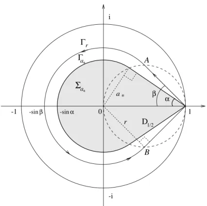
Dα := {z ∈ C : |z| ≤ sin α} ∪ {z ∈ C : | arg(1 − z)| ≤ α and |z − 1| ≤ cos α}. This is a convex subset of the unit disc Dr=1, with ”angle” (in contrast to tangent) touching of its boundary ∂Dr=1 at only one point z = 1, see Figure 1. It is evident that Dα ⊂ Dβ>α.
Definition 2.2 (Quasi-Sectorial Contractions [4]) A contraction C on the Hilbert space H is called quasi-sectorial with semi-angle α ∈ [0, π/2) with respect to the vertex at z = 1, if N(C) ⊆ Dα.
Notice that if operator C is a quasi-sectorial contraction, then I − C is an m-sectorial operator with vertex z = 0 and semi-angle α. The limits α = 0 and α = π/2 correspond, respectively, to non-negative (i.e. self-adjoint) and to general contraction.
The resolvent of an m-sectorial operator A, with semi-angle α ∈ (0, π/4] and vertex at z = 0, gives the first non-trivial (and for us a key) example of a quasi-sectorial contraction.
Proposition 2.1 Let A be m-sectorial operator with semi-angle α ∈ [0, π/4] and vertex at z = 0. Then {F (t) := (I +tA)−1}t≥0is a family of quasi-sectorial contractions which numerical ranges N(F (t)) ⊆ Dα for all t ≥ 0.
Proof : First, by virtue of Proposition 1.1 (ii) we obtain the estimate: kF (t)k ≤ 1
t dist(1/t , −Sα)
= 1 , (2.1)
which implies that operators {F (t)}t≥0are contractions with numerical ranges N(F (t)) ⊆ Dr=1.
Next, by Remark 1.2 for all u ∈ H one gets (u, F (t)u) = (vt, vt) + t(Avt, vt) ∈ Sα, where vt := F (t)u, i.e. for any t ≥ 0 the numerical range N(F (t)) ⊆ Sα. Similarly, one finds that (u, (I − F (t))u) = t(v, Av) + t2(Av, Av) ∈ Sα, i.e., N(I − F (t)) ⊆ Sα. Therefore, for all t ≥ 0 we obtain:
N(F (t)) ⊆ (Sα∩ (1 − Sα)) ⊂ Dr=1 . (2.2)
Moreover, since α ≤ π/4, by Definition 2.1 we get (Sα∩ (1 − Sα)) ⊂ Dα, i.e. for these values of α the operators {F (t)}t≥0 are quasi-sectorial contractions
with numerical ranges in Dα. ¤
Now we are in position to prove the main Theorem establishing a relation be-tween quasi-sectorial contraction semigroups and a certain class of m-sectorial generators.
Theorem 2.1 Let A be an m-sectorial operator with semi-angle α ∈ [0, π/4] and with vertex at z = 0. Then {e−t A}
t≥0 is a quasi-sectorial contraction semigroup with numerical ranges N(e−t A) ⊆ Dα for all t ≥ 0.
The proof of the theorem is based on a series of lemmata and on the numerical range mapping theorem by Kato [8] (see also an important comment about this theorem in [10]).
Proposition 2.2 [8] Let f (z) be a rational function on the complex plane C, with f (∞) = ∞. Let for some compact and convex set E′ ⊂ C the inverse function f−1 : E′ 7→ E ⊇ K, where K is a convex kernel of E, i.e., a subset of E such that E is star-shaped relative to any z ∈ K.
If C is an operator with numerical range N(C) ⊆ K, then N(f (C)) ⊆ E′. Notice that for a convex set E the corresponding convex kernel K = E. Lemma 2.1 Let fn(z) = zn be complex functions, for z ∈ C and n ∈ N. Then the sets fn(Dα) are convex and domains fn(Dα) ⊆ Dα for any n ∈ N, if α ≤ π/4.
Lemma 2.2 (Euler formula) Let A be an m-sectorial operator. Then for t ≥ 0 one gets the strong limit
s − lim
n→∞(F (t/n))
n= e−tA . (2.3)
The next section is reserved for the proofs. They refine and modify some lines of reasonings of the paper [4]. This concerns, in particular, a corrected proofs of Proposition 2.1 and Theorem 2.1 (cf. Theorem 2.1 of [4]), as well as reformulations and proofs of Propositions 2.2 and Lemma 2.1.
3 Proofs
Proof (Lemma 2.1):
Let {z : |z| ≤ sin α} ⊂ Dα, then one gets |zn| ≤ sin α. Therefore, for the mappings fn: z 7→ zn one obtains fn(z) ∈ Dα for any n ≥ 1.
Thus, it rests to check the same property only for images fn(Gα), n ≥ 1 of the sub-domain:
Gα := {z : | arg(z)| < (π/2 − α)} ∩ {z : | arg(z + 1)| > (π − α)} ⊂ Dα, (3.1) see Definition 2.1 and Figure 1.
For 0 ≤ t ≤ cos α, two segments of tangent straight intervals: {ζ±(t) = 1 + t ei(π∓α)}0≤t≤cos α ⊂ ∂Dα,
are correspondingly upper ζ+(t) and lower ζ−(t) = ζ+(t) non-arc parts of the total boundary ∂Dα; they also coincide with a part of the boundary ∂Gα connected to the vertex z = 1.
Now we proceed by induction. Let n = 1. Then one obviously obtain : fn=1(Dα) = Dα. For n = 2 the boundary ∂f2(Gα) of domain f2(Gα) is a union Γ2(α) ∪ Γ2(α) of the contour
Γ2(α) := {f2(ζ+(t))}0≤t≤cos α∪ {z : |z| ≤ sin2α, arg(z) = (π − 2α)} and its conjugate Γ2(α). Since arg(∂tf2(ζ+(t)) ≤ (π − α) for all 0 ≤ t ≤ cos α, the contour
{f2(ζ+(t))}0≤t≤cos α ⊆ {z : | arg(z + 1)| > (π − α)},
see (3.1). The same is obviously true for the image of the lower branch ζ−(t). If α ≤ π/4, one gets:
sup
0≤t≤cos αIm(f2(ζ+(t))) = Im(f2(ζ+(t
∗ = (2 cos α)−1))) (3.2) =1
2tan α < sin α cos α , where t∗ = (2 cos α)−1 ≤ cos α, and
0 ≥ Re(f2(ζ+(t))) ≥ − sin2α cos 2α ≥ − sin α .
Therefore, {f2(ζ+(t))}0≤t≤cos α ⊆ Dα. Since the same is also true for the im-age of the lower branch ζ−(t), we obtain f2(Gα) ⊂ Dα and by consequence fn=2(Dα) = {w = z · z : z ∈ Dα, z ∈ fn=1(Dα)} ⊂ Dα, for α ≤ π/4.
Now let n > 2 and suppose that fn(Dα) ⊂ Dα. Then the image of the (n+1) − order mapping of domain Dα is:
fn+1(Dα) = {w = z · zn: z ∈ Dα, zn∈ fn(Dα)},
and since fn(Dα) ⊂ Dα, we obtain fn+1(Dα) ⊂ Dα by the same reasoning as
for n = 2. ¤
Remark 3.1 Let φ(t) := arg(ζ+(t)). Then cot(α + φ(t)) = (cos α − t)/ sin α and sup 0≤t≤cos αIm(fn(ζ+(t))) ≤ (1 − 2t ∗ ncos α + (t∗n)2)n/2 (3.3) for sin(nφ(t∗
n)) = 1. In the limit n → ∞ this implies that φ(t∗n) = π/2n + o(n−1), t∗
n = π/(2n sin α) + o(n−1) and lim
n→∞0≤t≤cos αsup Im(fn(ζ+(t))) ≤ exp(− 1
2π cot α) < 1
2tan α. (3.4)
By the same reasoning one gets the estimates similar to (3.3) and (3.4) for ζ−(t)). Hence, |Im(fn(ζ±(t)))| < Im(fn=1(ζ+(t))) < sin α cos α, cf. (3.2). Notice that in spite of the arc-part of the contour ∂Dα shrinks in the limit n → ∞ to zero, we obtain
lim
n→∞0≤t≤cos αsup Re(fn(ζ+(t))) = − exp(−π cot α), (3.5)
for the left extreme point of the projection on the real axe (sin(nφ(t∗
n)) = 1) of the image fn(Dα). Since exp(−π cot α) < sin α, for α ≤ π/4, the arguments (3.4) and (3.5) bolster the conclusion of the Lemma 2.1.
Proof (Lemma 2.2): By (2.1) we have for λ > 0
k(λI + A)−1k < λ−1 , (3.6) and since A is m-sectorial, we also get that (−∞, 0) ⊂ ρ(A). Then the Hille-Yosida theory ensures the existence of the contraction semigroup {e−t A}t≥0, and the standards arguments (see e.g. [7, Ch.V], or [11, Ch.1.1]) yield the convergence of the Euler formula (2.3) in the strong topology. ¤ Proof (Theorem 2.1):
Take f (z) = z2 and the compact convex set E′ := f (Dα) ⊆ Dα, see Lemma 2.1. Since the set E := f−1(E′) = Dα∪ (−Dα) is convex, its convex kernel K exists and K = E. Then by Proposition 2.2 we obtain that N(f (C)) ⊆ E′ ⊆ Dα, if the numerical range N(C) ⊆ K.
Let contraction C1 := (I + t A/2)−1 = F (t/2). Since by Proposition 2.1 for any t ≥ 0 we have N(C1) ⊆ Dα and since Dα ⊂ E, we can choose K = E. Then by the Kato numerical range mapping theorem (Proposition 2.2) we get: N(f (C1) = F (t/2)2) ⊆ E′ ⊆ Dα . (3.7) Similarly, take the contraction C2 := F (t/4)2. Since (3.7) is valid for any t ≥ 0, it is true for t 7→ t/2. Then by definition of K one has N(F (t/4)2) ⊆ Dα ⊆ K. Now again the Proposition 2.2 implies:
N(f (C2) = F (t/4)4) ⊆ E′ ⊆ Dα . (3.8) Therefore, we obtain N(Fb(t/2n)2n
) ⊆ Dα, for any n ∈ N. By Lemma 2.2 this yields
lim
n→∞(u, (I + t A/2 n)−2n
u) = (u, e−t Au) ∈ Dα ,
for any unit vector u ∈ H. Therefore, the numerical ranges of the contraction semigroup N(e−t A) ⊆ Dαfor all t ≥ 0, if it is generated by m-sectorial operator with the semi-angle α ∈ [0, π/4] and with the vertex at z = 0. ¤
4 Corollaries and Applications
1. Notice that Definition 2.2 of quasi-sectorial contractions C is quite restric-tive comparing to the notion of general contractions, which demands only N(C) ⊆ D1. For the latter case one has a well-known Chernoff lemma [5]:
which is not even a convergent bound. For quasi-sectorial contractions we can obtain a much stronger estimate [4]:
° ° °C n− en(C−I)° ° ° ≤ M n −1/3 , n ∈ N , (4.2)
convergent to zero in the uniform topology when n → ∞. Notice that the rate of convergence n−1/3 obtained in [4] with help of the Poisson representation and the Tchebychev inequality is not optimal. In [9], [2] and [1] this estimate was improved up to the optimal rate O(n−1), which one can easily verify for a particular case of self-adjoint contractions (i.e. α = 0) with help of the spectral representation.
The inequality (4.2) and its further improvements are based on the following important result about the upper bound estimate for the case of quasi-sectorial contractions:
Proposition 4.1 If C is a quasi-sectorial contraction on a Hilbert space H with semi-angle 0 ≤ α < π/2, i.e. the numerical range N(C) is a subset of the domain Dα, then
kCn(I − C)k ≤ K
n + 1 , n ∈ N . (4.3)
For the proof see Lemma 3.1 of [4].
2. Another application of quasi-sectorial contractions generalizes the Chernoff semigroup approximation theory [5], [6] to the operator-norm approximations [4].
Proposition 4.2 Let {Φ(s)}s≥0 be a family of uniformly quasi-sectorial con-tractions on a Hilbert space H, i.e. such that there exists 0 < α < π/2 and N(Φ(s)) ⊆ Dα, for all s ≥ 0. Let
X(s) := (I − Φ(s))/s ,
and let X0 be a closed operator with non-empty resolvent set, defined in a closed subspace H0 ⊆ H. Then the family {X(s)}s>0 converges, when s → +0, in the uniform resolvent sense to the operator X0 if and only if
lim n→∞ ° ° °Φ(t/n) n− e−tX0 P0°° °= 0 , for t > 0 . (4.4)
Here P0 denotes the orthogonal projection onto the subspace H0.
3. We conclude by application of Theorem 2.1 and Proposition 4.1 to the Euler formula [4], [9], [2].
Proposition 4.3 If A is an m-sectorial operator in a Hilbert space H, with semi-angle α ∈ [0, π/4] and with vertex at z = 0, then
lim n→∞ ° ° °(I + tA/n) −n− e−tA°° °= 0, t ∈ Sπ/2−α.
Moreover, uniformly in t ≥ t0 > 0 one has the error estimate:
° ° °(I + tA/n) −n− e−tA° ° °≤ O ³ n−1´ , n ∈ N . Acknowledgements
I would like to thank Professor Mitsuru Uchiyama for a useful remark indi-cating a flaw in our arguments in Section 2 of [4] , revision of this part of the paper [4] is done in the present manuscript. I also thankful to Vincent Cachia and Hagen Neidhardt for a pleasant collaboration.
References
[1] V. Bentkus and V. Paulauskas, Optimal error estimates in operator-norm approximations of semigroups. Lett. Math. Phys. 68 (2004), 131–138.
[2] V. Cachia, Euler’s exponential formula for semigroups, Semigroup Forum 68 (2004), 1–24.
[3] V. Cachia, H. Neidhardt, V.A. Zagrebnov, Comments on the Trotter product formula error-bound estimates for nonself-adjoint semigroups, Integral Equat.
Oper. Theory 42 (2002), 425–448.
[4] V. Cachia, V.A. Zagrebnov, Operator-norm approximation of semigroups by quasi-sectorial contractions, J. Funct. Anal. 180 (2001), 176–194.
[5] P.R. Chernoff, Note on product formulas for operator semigroups. J. Funct.
Anal. 2 (1968) 238–242.
[6] P.R. Chernoff, Product formulas, nonlinear semigroups, and addition of
unbounded operators. Memoirs of the American Mathematical Society, No.
140. American Mathematical Society, Providence, R. I., 1974.
[7] T. Kato, Perturbation Theory for Linear Operators, Springer-Verlag, Berlin, 1966.
[8] T. Kato, Some mapping theorems for the numerical range, Proc. Japan Acad. 41(1966), 652–655.
[9] V. Paulauskas, On operator-norm approximation of some semigroups by quasi-sectorial operators, J. Funct. Anal. 207 (2004), 58–67.
[10] M. Uchiyama, Numerical ranges of elements of involutive Banach algebras and commutativity, Arch.Math. 69 (1997), 313–318.
[11] V.A. Zagrebnov, Topics in the theory of Gibbs semigroups. Leuven Notes in Mathematical and Theoretical Physics. Series A: Mathematical Physics, 10. Leuven University Press, Leuven, 2003.
-1 -sin 1 Γ Γa β β r α α 1/2 D B a * * a* i -i 0 A
Σ
r -sinFig. 1. Illustration of the set Dα(= Σa∗ shaded domain) with boundary ∂Dα = Γa∗, where a∗ = sin α, as well as of our choice of the contour Γrin the resolvent set ρ(C),
where r = sin β > a∗. The contour Γr consists of two segments of tangent straight
lines (1, A) and (1, B) and the arc (A, B) of radius r. The dotted circle ∂Dr=1/2