A Deep Neural Network for Simultaneous
Estimation of b Jet Energy and Resolution
The MIT Faculty has made this article openly available.
Please share
how this access benefits you. Your story matters.
Citation
Sirunyan, A. M. et al. "A Deep Neural Network for Simultaneous
Estimation of b Jet Energy and Resolution." Computing and
Software for Big Science 4, 10 (October 2020): doi.org/10.1007/
s41781-020-00041-z. © 2020 The Author(s)
As Published
https://doi.org/10.1007/s41781-020-00041-z
Publisher
Springer International Publishing
Version
Final published version
Citable link
https://hdl.handle.net/1721.1/129404
Terms of Use
Creative Commons Attribution
https://doi.org/10.1007/s41781-020-00041-z
ORIGINAL ARTICLE
A Deep Neural Network for Simultaneous Estimation of b Jet Energy
and Resolution
CMS Collaboration193
Received: 24 December 2019 / Accepted: 20 June 2020 / Published online: 30 October 2020 © The Author(s) 2020
Abstract
We describe a method to obtain point and dispersion estimates for the energies of jets arising from b quarks produced in proton–proton collisions at an energy of √s = 13 TeV at the CERN LHC. The algorithm is trained on a large sample of
simulated b jets and validated on data recorded by the CMS detector in 2017 corresponding to an integrated luminosity of 41 fb−1 . A multivariate regression algorithm based on a deep feed-forward neural network employs jet composition and shape
information, and the properties of reconstructed secondary vertices associated with the jet. The results of the algorithm are used to improve the sensitivity of analyses that make use of b jets in the final state, such as the observation of Higgs boson decay to b̄b.
Keywords CMS · b jets · Higgs boson · Jet energy · Jet resolution · Deep learning
Introduction
Following the discovery of the 125 GeV Higgs boson reported by the ATLAS and CMS Collaborations at the CERN LHC in 2012[1–3], a rich research program was established to probe this new particle. The program includes the measurement of all production and decay modes that are accessible at the LHC. The decay of the Higgs boson into a pair of vector bosons was established with a statistical sig-nificance higher than five standard deviations individually for photon, Z and W pairs using data collected at the LHC from 2011 to 2013 at center-of-mass energies of √s = 7
and 8 TeV[4–9]. A few years later, the combination of CMS data sets collected at 8 and 13 TeV was used to report the observation of Higgs boson decay to a pair of 𝜏 leptons[10], followed by the observation of the associated production of a Higgs boson with a top quark–antiquark pair ( t̄t)[11, 12].
Higgs boson decay to a b quark–antiquark pair ( b̄b ) was only recently announced by the CMS[13] and ATLAS[14] collaborations, despite it being the dominant decay mode. This is because of the challenges associated with separating the signal from the large background of b̄b produced by quan-tum chromodynamics (QCD) processes. Good resolution of
the reconstructed invariant mass of Higgs boson candidates is necessary to have a more favorable signal-to-background ratio. This is achieved in CMS by the method described in this paper, based on a deep neural network (DNN) that esti-mates the energy of jets originating from b quarks (b jets). Similar algorithms, using neural networks, were previously used by the CDF Collaboration at the Tevatron [15, 16], and BDT-based energy regressions were used earlier by the CMS Collaboration to estimate the energy of b jets[17].
The approach described in this paper is to use a regres-sion algorithm that is implemented in a feed-forward neural network with six hidden layers trained on a very large data set, consisting of Monte Carlo (MC) simulated b jets. The algorithm has a considerably larger modeling capability than those used previously. This approach was made possible by leveraging recent advances in hardware accelerators, such as graphics processing units (GPU), and in modern pack-ages for automatic differentiation to handle the otherwise expensive computations involved in this task. A minimi-zation of a loss function that combines a Huber [18] and two quantile [19] loss terms enables simultaneous training of point and dispersion estimators of the regression target without making any assumptions about the functional form of its distribution. The point estimator is used as a correc-tion of the measured b jet energy, while dispersion estima-tors are used to build a jet-by-jet resolution estimate. The Deceased: A. M. Sirunyan, G. Vesztergombi, S. Guts, G. R. Snow
CMS collaboration had previously developed a BDT-based approach to estimate the energy and per-object resolution [20–22]. This can be achieved by training separate regres-sions to obtain energy and per-object resolution estimators, or by means of a semiparametric regression [20, 21]. For a semiparametric regression, the training relies on the knowl-edge of the analytical shape of the target distribution. The novel characteristic of the algorithm described in this paper is the simultaneous training of the point and dispersion esti-mators without reference to an ansatz distribution for the regression target. This method is validated on data collected by the CMS detector in 2017.
In the following, Sect. 2 and Sect. 3 describe the CMS detector and the data sets used for this work. The regression problem and the inputs are described in Sect. 4. In Sect. 5, the loss function is introduced, while the DNN architecture and its training are summarized in Sect. 6. Finally, the results are presented in Sect. 7, followed by the summary in Sect. 8.
The CMS Detector
The central feature of the CMS detector is a superconducting solenoid of 6 m internal diameter, providing a magnetic field of 3.8 T. Within the solenoid volume are a silicon pixel and strip tracker, a lead tungstate crystal electromagnetic rimeter (ECAL), and a brass and scintillator hadron calo-rimeter (HCAL), each composed of a barrel and two endcap sections. Forward calorimeters extend the pseudorapidity ( 𝜂 ) coverage provided by the barrel and endcap detectors. Muons are detected in gas-ionization chambers embedded in the steel flux-return yoke outside the solenoid. A detailed description of the apparatus, together with a definition of the coordinate system used and the relevant kinematic variables, can be found in Ref.[23].
The particle-flow (PF) algorithm [24] used by CMS aims to reconstruct and identify each individual particle in an event, with an optimized combination of information from the various elements of the CMS detector. Photon energies are obtained from ECAL data. The candidate vertex with the largest value of summed physics-object p2
T is taken to
be the primary proton–proton ( pp ) interaction vertex. The energy of each electron in the event is determined from a combination of the electron momentum at the primary inter-action vertex, as determined by the tracker, the energy of the corresponding ECAL cluster, and the energy sum of all bremsstrahlung photons spatially compatible with having originated from the electron. The momentum of each muon is obtained via the curvature of the corresponding track. The energy of each charged hadron is determined from a combination of momentum measured in the tracker and the matching ECAL and HCAL energy deposits, corrected for
zero-suppression effects and for the response function of the calorimeters to hadronic showers. Finally, for a neutral had-ron, the energy is obtained from the corresponding HCAL corrected energies. The anti-kT algorithm [25, 26] with a
distance parameter of 0.4 is applied offline to the full set of PF candidates to cluster them into jets. The jet momentum is determined by the vectorial sum of all particle momenta in the jet. The jet energy resolution typically amounts to 15–20% at 30 GeV , 10% at 100 GeV , and 5% at 1 TeV[27].
Additional pp interactions within the same or nearby bunch crossings (pileup) can contribute unrelated particles to the jet. To mitigate the effects of pileup, charged particles with tracks originating from pileup vertices are discarded before jet reconstruction. Then, the residual contamination from neutral particles and charged particles without reconstructed tracks is estimated for each event and subtracted from the jet energy. Jet energy corrections are derived from simulation to bring the measured average response for jets in line with particle-level jets. Neutrinos are not included in the clustering of particle-level jets. In situ measurements of the transverse momentum balance in dijet, photon+jet, Z+jet, and multijet events are used to account for residual differences between the jet energy scales in data and simulation[28]. We refer to this correction algorithm as the baseline algorithm.
Data Sets
The DNN was trained on 100 million b jets from a sim-ulated sample of t̄t events produced in pp collisions at √
s = 13 TeV , generated at next-to-leading-order (NLO)
accuracy in perturbative QCD (pQCD) with the powheg v2
program[29]. Predictions of the model were then tested on simulated events with b jets coming from a variety of physical processes to validate performance in all relevant kinematic regions. To this end, b jets from the decay of Higgs bosons produced in association with a Z boson, Z(→ 𝓁+𝓁−
)H(→ b ̄b) , where 𝓁 is an electron or a muon, were generated with the Madgraph 5_aMc@nlo generator[30] at
NLO pQCD accuracy. Additionally, b jets from the decay of Higgs boson pairs produced either from gluon fusion or in the decay of a new, spin-0 resonance, with one Higgs boson decaying to a b quark-antiquark pair and the other to a pair of photons, H(→ b̄b)H(→ γγ) , were generated with Madgraph
5_aMc@nlo at leading-order accuracy in pQCD.
Two definitions of jets are used in this study: “genera-tor-level jets”, clustered from stable particles produced by the MC generator that include the contribution from the neutrino’s momentum, and “reconstructed jets”, clus-tered from reconstructed particle-flow candidates. The reconstructed b jets were matched to generated b jets to avoid contamination by light flavored jets. For each recon-structed jet, the corresponding generator-level jet is found
by spatial matching in the 𝜂 − 𝜙 plane by requiring the dis-tance 𝛥R =√(𝛥𝜂)2+ (𝛥𝜙)2 (where 𝜙 is the azimuthal angle in radians) to be 𝛥R < 0.4 . The reconstructed b jets were then selected by applying a minimum threshold for trans-verse momentum ( preco
T > 15 GeV , p gen
T > 15 GeV ) and by
requiring the pseudorapidity of the central axis of the recon-structed jet to be within the tracker acceptance ( |𝜂| < 2.4).
Finally, to validate the regression model on data, the output of the DNN for simulated b jets was compared to that obtained for b jets recorded by the CMS detector. The events used for this validation were recorded in 2017 with triggers[31] that require the presence of at least one lepton. This data set, cor-responding to an integrated luminosity of 41 fb−1 , was
fur-ther enriched in Z bosons produced in association with b jets. The corresponding simulated events come from a sample of Z bosons and up to two additional partons generated with Madgraph 5_aMc@nlo at NLO accuracy in pQCD.
For all simulated events, pythia 8.2[32] with the CP5
tune[33] is used for parton showering and hadronization. The CMS detector response is simulated by the geant4[34]
package, and simulated pileup interactions are added to the hard-scattering process to match the distribution of pileup interactions observed in data, for which the observed mean number of interactions per bunch crossing is 32.
Energy Regression and Input Features
In comparison to jets arising from light-flavor quarks or gluons, jets arising from b quarks have special characteristics that call for dedicated energy corrections. In particular, b jets contain b hadrons that can often decay to a final state with a charged lepton and a neutrino. The neutrinos, which only inter-act via the weak force, escape detection, leading to an under-estimate of the b jet energy, with a corresponding degradation of energy resolution. As described in Sect. 2, the jet energy is reconstructed by clustering its constituents within a given dis-tance parameter. Compared to jets originating from light-flavor quarks and gluons, b jets, because of their higher mass, tend to spread radially over a wider area in the 𝜂-𝜙 plane. This often leads to leakage of energy outside of the jet clustering region, further impacting the jet energy response and resolution.
The b jets used for the DNN training come from a sample of simulated top quark events. The top quark decays before had-ronising with a branching fraction close to unity into a b jet and a W boson. At LHC energies, it provides a source of b jets that spans a large transverse momentum ( pT ) spectrum and covers
the full 𝜂 acceptance of the detector. The preco
T value is corrected
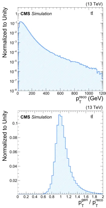
with the baseline algorithm as described in Sect. 2. Figure 1
(upper) shows the distribution of preco
T , for the selected b jets.
The regression target, y, used in this study is defined as the ratio of the transverse momentum of the generator-level jet, pgen
T , to that of the reconstructed jet, p reco
T , applying the
baseline jet energy corrections. Using this definition rather than using pgen
T directly has the effect of greatly reducing the
variance of the target while producing a numerical value of order 1. The distribution of the target for b jets from an MC simulated t̄t sample is shown in Fig. 1 (lower). To improve the convergence of the training of the DNN, the target is further standardized by subtracting its median value and dividing it by its standard deviation.
The DNN training inputs provide information about the kinematics, shape, and composition of reconstructed jets. The inputs consist of the following features:
(GeV)
reco Tp
0 200 400 600 800 1000 1200Normalized to Unity
8 − 10 7 − 10 6 − 10 5 − 10 4 − 10 3 − 10 2 − 10 1 − 10 1 CMS Simulation (13 TeV) tt reco T/ p
gen Tp
0 0.2 0.4 0.6 0.8 1 1.2 1.4 1.6 1.8 2Normalized to Unity
0.02 0.04 0.06 0.08 0.1 CMS Simulation (13 TeV) ttFig. 1 (upper) The preco
T distribution for reconstructed b jets in an MC
t̄tsample. (lower) Distribution of the regression target for the MC t̄t training sample
– jet kinematics: jet pT , 𝜂 , mass, and transverse mass,
defined as √E2
− p2z;
– information about pileup interactions: the median energy density in the event, 𝜌 , corresponding to the amount of transverse momentum per unit area that is due to overlap-ping collisions[35];
– information about semileptonic decays of b hadrons when an electron or muon candidate is clustered within a jet: the transverse component of lepton momentum perpen-dicular to the jet axis, the distance 𝛥R =√(𝛥𝜂)2+ (𝛥𝜙)2 , and a categorical variable that encodes information about the lepton candidate’s flavor;
– information about the secondary vertex, selected as the highest pT displaced vertex linked to the jet: number of
tracks associated to the vertex, transverse momentum, and mass (computed assigning the pion mass to all reconstructed tracks forming the secondary vertex); the
distance between the collision vertex and the second-ary vertex computed in three-dimensional space with its associated uncertainty[36, 37];
– jet composition: largest pT value of any charged hadron
candidates, fractions of energy carried by jet constituents; namely charged hadrons, neutral hadrons, muons, and an electromagnetic component coming from electrons and photons. These fractions are computed for the whole jet, and separately in five rings of 𝛥R around the jet axis ( 𝛥R = 0–0.05, 0.05–0.1, 0.1–0.2, 0.2–0.3, 0.3–0.4); – multiplicity of PF candidates clustered to form the jet; – information about jet energy sharing among the jet
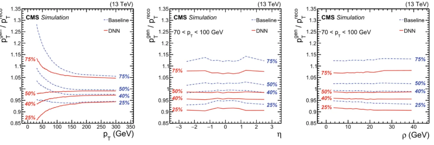
con-stituents computed as (1) �∑ ip2T,i ∑ ipT,i , (GeV) T p 0 50 100 150 200 250 300 350 reco T / p gen p T 0.85 0.9 0.95 1 1.05 1.1 1.15 1.2 1.25 1.3 1.35 Baseline DNN 25% 40% 50% 75% 25% 40% 50% 75% CMS Simulation (13 TeV) 3 − −2 −1 0 1 2 3 η 0.85 0.9 0.95 1 1.05 1.1 1.15 1.2 1.25 1.3 1.35 reco T / p gen p T Baseline DNN 25% 40% 50% 75% 25% 40% 50% 75% CMS Simulation (13 TeV) < 100 GeV T 70 < p 0 10 20 30 40 (GeV) ρ 0.85 0.9 0.95 1 1.05 1.1 1.15 1.2 1.25 1.3 1.35 reco T / p gen p T Baseline DNN 25% 40% 50% 75% 25% 40% 50% 75% CMS Simulation (13 TeV) < 100 GeV T 70 < p
Fig. 2 The 25, 40, 50, and 75% quantiles are shown for the b jet energy scale pgen
T ∕p reco
T distribution before (blue dashdot) and after
(red solid) applying the regression correction as a function of jet pT
(left), 𝜂 (center), and 𝜌 (right). The 𝜂 and 𝜌 distributions are shown for jets with pT ∈ [70, 100] GeV
0.06 0.08 0.1 0.12 0.14 0.16 0.18 s Baseline DNN CMS Simulation (13 TeV) 0 50 100 150 200 250 300 350 400 (GeV) gen T p 0 0.1 0.2 baseline s s∆ 0.06 0.08 0.1 0.12 0.14 0.16 0.18 s Baseline DNN CMS Simulation (13 TeV) < 100 GeV T 70 < p 0 0.5 1 1.5 2 2.5 | η | 0 0.1 0.2 baseline s s∆ 0.06 0.08 0.1 0.12 0.14 0.16 0.18 s Baseline DNN CMS Simulation (13 TeV) < 100 GeV T 70 < p 0 5 10 15 20 25 30 35 40 45 (GeV) ρ 0 0.1 0.2 baseline s s∆
Fig. 3 Relative jet energy resolution, s , as a function of generator-level jet pgen
T (left), 𝜂 (center), and 𝜌 (right) for b jets from t̄t MC
events. The average pT of these b jets is 80 GeV . The 𝜂 and 𝜌
distribu-tions are shown for jets with pT ∈ [70, 100] GeV . The blue stars and
red squares represent s before and after the DNN correction, respec-tively. The relative difference 𝛥s∕sbaseline between the s values before
where i runs over all jet constituents.
This results in a total of 41 input features. No additional preprocessing is performed, apart from the input normaliza-tion provided by batch normalizanormaliza-tion[38] at the input layer of the DNN.
Loss Function
A possible approach to such a regression problem is to develop separate dedicated regressions to obtain energy and per-object resolution estimators. If the target distribution can be parametrized analytically, one can use a semiparametric regression to obtain estimates of the function parameters. This method has been used by the CMS collaboration to estimate the energy and resolution of electron and photon candidates[20, 21]. Whereas for the photon and electron candidates, the energy response can be parametrized by an analytically integrable function, this is less straightforward for b jets, making such an approach to the problem more expensive computationally. An alternative approach is to simultaneously obtain point and dispersion estimates of the b jet energy by defining a loss function that is completely agnostic to the target distribution. The correction to be applied to the reconstructed b jet energy can be obtained as the estimated mean, while the per-jet b jet energy resolution can be estimated as half the difference of the 75 and 25% quantiles. Therefore, the regression loss function should pro-vide the mean estimator ( ̂y ), and the 25 and 75% quantiles of the target distribution.
The Huber loss function is employed to learn the mean of the target distribution via a minimization process. It is pref-erable to the mean squared error because of its reduced sen-sitivity to the tails of the target distribution. It is defined as:
where z = y − ̂y , and 𝛿 is set to 1 in our case. To estimate the 25 and 75% quantiles of the target distribution, the quantile loss function is used:
where 𝜏 = 0.25 (0.75) corresponds to the 25 (75)% quantile. The complete loss function can then be written as:
where E(x,y)∼p(x,y) denotes the expectation value when
sam-pling (x, y) on the distribution p(x, y), x denotes the set of (2) H𝛿(z) = {1 2z 2, if|z| < 𝛿; 𝛿|z| −12𝛿2, otherwise, (3) 𝜌𝜏(z) = { 𝜏z, if z > 0; (𝜏 − 1)z, otherwise, (4) loss(̂y, ̂y25%, ̂y75%) = E(x,y)∼p(x,y)[H1(y − ̂y(x))
+ 𝜌0.25(y − ̂y25%(x))
+ 𝜌0.75(y − ̂y 75%(x))],
input features, and p(x, y) is the joint distribution of the input features and the target variables y in the training sample. The symbols ̂y(x) , ̂y25%(x) , and ̂y75%(x) denote the DNN outputs: ̂y(x) is the mean estimator, and ̂y25%(x) and ̂y75%(x) are the 25
and 75% quantile estimators, respectively.
Neural Network Architecture
The model used for this study is a feed-forward, fully con-nected DNN with 6 hidden layers, 41 input features, and 3 outputs: the energy correction and the 25 and 75% quantiles. As mentioned above, a batch normalization layer is applied at the DNN input.
Each hidden layer of the DNN is built from the following components:
– Dense layer: defined as a linear combination of all out-puts from the previous layer.
– Batch normalization layer: to transform the inputs to zero-mean and unit-variance.
– Dropout unit: an operation that zeroes a fixed fraction of randomly chosen nodes during the training, used as a regularization handle. The dropout rate is one of the optimized hyperparameters of the DNN.
– Activation unit: we chose the “Leaky” Rectified Linear Unit (LReLU)[39]:
with 𝛽 = 0.2.
A small slope 𝛽 = 0.2 was chosen for the LReLU to allow for a nonvanishing gradient over the domain of the function [39]. The output layer has a linear activation function. The DNN is implemented using the Keras package [40] with
tensorFlow backend [41]. Back-propagation is done using
stochastic gradient descent with the Adam optimizer [42]. Hyperparameter Optimization
To optimize the performance of the DNN, three hyperparam-eters are considered: the depth of the network architecture, the dropout rate, and the gradient descent learning rate. They were tuned using the cross-validation algorithm [43]. The mean vali-dation loss was used as the figure of merit for the optimization over a five-fold splitting of the training sample. The network has been trained on a single NVIDIA GeForce GTX 1080 Ti GPU.
Random sampling was used to select 50 of 120 grid points in hyperparameter space, where the grid is defined by the following: – dropout rate: do ∈ [0.1, 0.2, 0.3, 0.4]. (5) LReLU(x) = { x, if x ≥ 0; 𝛽x, if x < 0,
– learning rate: lr ∈ [10−2, 10−3, 10−4, 10−5, 10−6].
– number of hidden layers: varied between 3 and 8. The number of nodes in the last three hidden layers of the DNN was set to [512, 256, 128], respectively, while the number of nodes of the remaining layers was set to 1024. A number of configurations were found to provide comparable performance. Of these, the network with the smallest num-ber of trainable parameters was chosen. The parameters and their values are: do = 0.1 , lr = 0.001 , and 6 hidden layers with [1024, 1024, 1024, 512, 256, 128] nodes. This archi-tecture has a total of about 2.8 million trainable parameters. Training Set pT Composition
The number of events as a function of the b jet pT spectrum
in the training sample spans six orders of magnitude, as shown in Fig. 1 (upper). This means that, during the train-ing, the DNN is exposed to many more jets with low pT .
In situations like this, one might expect worse performance for high-pT jets. To check if this is an issue, emphasis was
given to the high pT part of the sample. About 95% of the
jets with pT below 400 GeV were removed to reproduce the
same exponential shape observed above 400 GeV . We found that the DNN trained on this subsample of events showed no improvement for high pT jets, but did have up to 0.5%
degradation of the relative jet energy resolution. For this reason, the final DNN is trained on the full sample.
Results
The performance of the b jet regression was evaluated by comparing the b jet energy resolution and scale (defined as the most probable value of the pgen
T ∕p reco
T distribution),
before and after the energy correction, on a test sample that is statistically independent from those used for training and validation. Different physics processes were included in the test set to evaluate the performance of the algorithm on b jets with different kinematics. The processes employed in the test sample are:
– t̄t : top quark–antiquark pair production (independent of the training data set),
– Z(→ 𝓁+𝓁−)H(→ b ̄b) : associated production of a Higgs
boson with a Z boson, where the Z boson decays to a pair of same flavor, opposite-charge electrons or muons, and the Higgs boson decays to b̄b,
– H(→ b̄b)H(→ γγ) : double Higgs boson produced via gluon fusion with one Higgs boson decaying to b̄b , and the other to a pair of photons, assuming both standard model (SM) and beyond SM kinematics. In the latter case, the double Higgs signal originates from the decay of a spin-0 resonance with a mass of 500 or 700 GeV. Figure 2 shows the 25, 40, 50, and 75% quantiles of the target distribution before and after applying the DNN b jet energy corrections, as a function of jet pT , 𝜂 , and 𝜌 . The results are
obtained for b jets from the t̄ttest sample. The 40% quantile has been found to be a good approximation of the most probable value of the target distribution. In addition, the 40% quantile validates the performance on a quantile not used in the train-ing. It can be seen that after DNN corrections, the distribution becomes narrower, and its median and 40% quantile exhibit smaller dependence on jet pT , 𝜂 , and the median event energy
density 𝜌.
Table 1 Relative differences 𝛥s∕sbaseline between the s values obtained
before and after applying the DNN energy correction for b jets pro-duced in the different physics processes indicated
MC sample Improvement t̄t 12.2% Z(→ 𝓁+𝓁−)H(→ b ̄b) 12.8% H(→ b̄b)H(→ γγ) SM 13.1% H(→ b̄b)H(→ γγ) resonant 500 GeV 14.5% H(→ b̄b)H(→ γγ) resonant 700 GeV 13.1%
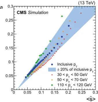
>
s
<
0 0.05 0.1 0.15 0.2 0.25 0.3s
0 0.05 0.1 0.15 0.2 0.25 0.3 CMS Simulation (13 TeV) T Inclusive p T 20% of inclusive p ± < 50 GeV T 30 < p < 70 GeV T 50 < p < 120 GeV T 110 < pFig. 4 Correlation between jet energy resolution s and the average jet energy resolution estimator ⟨̂s⟩ for b jets from t̄t MC events. The blue circles correspond to the inclusive pT spectrum, while the blue band
represents 20% up and down variations of the fitted ⟨̂s⟩ trend for the inclusive pT spectrum. The red stars correspond to jets with pT ∈ [30,
50] GeV , orange diamonds to pT ∈ [50, 70] GeV , and green crosses to pT ∈ [110,120] GeV
The jet energy resolution, s , is estimated as half the dif-ference between the 75% ( q75 ) and 25% ( q25 ) quantiles of the
target distribution. To quantify the resolution improvement, we compared the relative jet energy resolution, s , defined as:
where the resolution s is divided by q40 , the most probable
value estimated as the 40% quantile of the target distribu-tion. The relative improvement on s for b jets for various physics processes is between 12 and 15%, as can be seen from Table 1. Figure 3 shows the value of s obtained for b jets from the t̄t test sample as a function of the generator-level pgen
T (left), 𝜂 (center), and 𝜌 (right). The lower panels
in Fig. 3 show the relative improvements resulting from the DNN energy correction. The observed behavior agrees with the expectation that the regression correction should opti-mize the jet energy resolution, while the baseline corrections aim for a flat response as a function of the jet generator level
pgen
T and 𝜂 . For all physics processes considered, the
per-jet relative resolution improvement is around 12–18% for
pT < 100 GeV , falling to around 5–9% for pT > 200 GeV .
This improvement translates into an improvement in sensi-tivity of the analyses that make use of b jets in the final state. The improvement in the b jet energy resolution brought by the regression is similar for b jets with and without associ-ated leptons. This demonstrates that the algorithm is able to correct not only for the undetected neutrinos in semileptonic decays of b hadrons, but also for effects that may only be present in hadronic decays. In addition, the regression was shown to improve the response of light jets by about 3%.
Knowledge of jet energy resolution on a jet-by-jet basis can be exploited in analyses searching for resonant pro-duction of b jet pairs to increase their sensitivity. We have checked the correlation between the jet resolution s and the value of the per-jet resolution estimator, ̂s , provided by the DNN:
To do this, the sample of b jets was split into several equally populated bins in ̂s . In each bin, the value of s is computed as half the difference between the q75 and q25 quantiles of the
target distribution, and compared to the average resolution estimator ⟨̂s⟩ . Figure 4 shows the correlation between s and the ⟨̂s⟩ values for the inclusive pT spectrum and for several
bins in pT . A linear dependence with slope near unity
con-firms that the per-jet energy resolution estimator ̂s correctly represents the jet resolution. We observe that deviations of the slope from unity from the linear behavior are roughly compatible within 20% of the ̂s value.
(6) s ≡ s q40 = q75− q25 2 1 q40, (7) ̂s ≡1 2(̂y75%− ̂y25%).
While the improvements described above are quoted at the single jet level, many physics analyses use the invariant mass of the two b jet system as a discriminating variable for signal extraction. The improvement in the resolution of the dijet invariant mass is generally bigger than that for a single jet, because the energy corrections effectively equalize the energy scale of the two jets, while also improving the jet resolution. To estimate the dijet resolution, improvement, events with two leptons and two jets were selected from the Z(→ 𝓁+𝓁−
)H(→ b ̄b) sample: jets were required to have pT
larger than 20 GeV , absolute value of 𝜂 below 2.4, and be compatible with the hadronisation of b quarks, referred to as “b-tagged”[37] jets in the following. The selection crite-ria for the b-tagged jets correspond to a 70% b jet tagging efficiency with a 1% misidentification rate for light-flavor or gluon jets. Leptons were required to have a pT larger than
20 GeV , while the lepton pairs were required to be compat-ible with the decay of a Z boson, requiring their invariant mass to be within 20 GeV of the mass of the Z boson. The Z boson was required to have a transverse momentum larger than 150 GeV . An improvement of about 20% in the dijet invariant mass resolution in the Z(→ 𝓁+𝓁−
)H(→ b ̄b) sam-ple can be observed in Fig. 5. A Bukin function [44] was used to fit the core of the distribution in Fig. 5. The fit is performed in the range [75, 165] GeV for the baseline and [81,160] GeV for the DNN corrected distribution.
In addition, a dedicated study was performed to test how well the algorithm performance can be transferred from Monte Carlo simulations to the domain of pp collision data. A set of Z boson candidates decaying to a pair of charged leptons was extracted from pp collisions recorded by the CMS experiment in 2017. A standard set of requirements [28, 45] was applied to select events with electron or muon pairs compatible with having originated from the decay of a Z boson. Events were further required to have at least one b-tagged jet. The jet with the largest pT was required to have
|𝜂| < 2 , while the pT of the dilepton system was required to
be larger than 100 GeV . The pT balance between the Z boson
and the b-tagged jet candidate was enforced by requiring that extra jets have a pT less than 30% of the Z pT to suppress
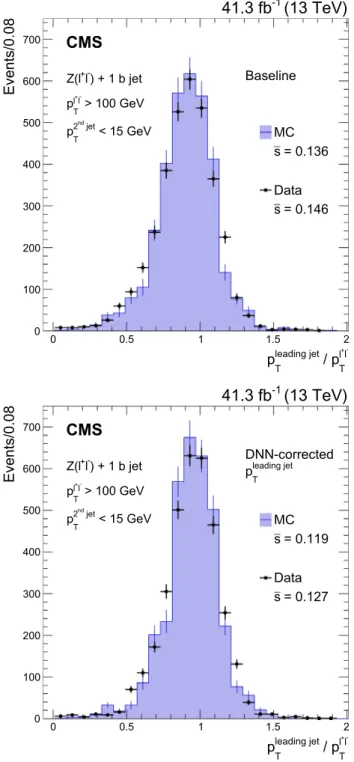
events with additional hadronic activity. Events satisfying these requirements were used to evaluate the agreement between data and MC simulations. In addition, the resolution of the jets was measured by extrapolating to zero additional hadronic activity following the methodology described in Ref. [28].
Figure 6 shows the ratio between the pT of the leading
jet and that of the dilepton system for events in which the
pT of the subleading jet is less than 15 GeV . The upper and
lower panels show the distributions obtained before and after applying the DNN-based corrections, respectively. It can be seen that the effect of the corrections is to reduce the width of the distribution. Using the method detailed in Ref. [28],
the double ratio of the relative jet resolution s measured in data and in simulated events was found to be 1.1 ± 0.1 before and after applying the DNN-based corrections. This vali-dates that the resolution improvement achieved in simulated events is successfully transferred to the data domain.
Summary
We have described an algorithm that makes it possible to obtain point and dispersion estimates of the energy of jets arising from b quarks in proton–proton collisions. We trained a deep, feed-forward neural network, with inputs based on jet composition and shape information, and on properties of the associated reconstructed secondary vertex for a sample of simulated b jets arising from the decays of top quark–anti-quark pairs. The neural network simultaneously finds robust mean, 25 and 75% quantile estimators for the energy of a b jet. The mean estimator is based on the Huber loss function and is used as an energy correction, while the 25 and 75% quantile estimators are used to build a jet-by-jet resolution estimator, defined as half the difference between these quantiles.
The DNN-based algorithm leverages the information contained in a large training data set consisting of nearly 100 million simulated b jets, and improves the resolution of
the b jet energy by 12–15% relative to that which is found after baseline corrections. An improvement of about 20% is observed in the resolution of the invariant mass of b jet pairs 0 20 40 60 80 100 120 140 160 (GeV) jj m 0 1 2 3 4 5 Entries / 5 GeV DNN = 15.4 GeV σ = 124.6 GeV µ Baseline = 18.0 GeV σ = 115.9 GeV µ CMS Simulation (13 TeV)
Fig. 5 Dijet invariant mass distributions for simulated samples of Z(→ 𝓁+𝓁−)H(→ b ̄b) events, where two jets and two leptons were
selected. Distributions are shown before (dotted blue) and after (solid red) applying the b jet energy corrections. A Bukin function [44] was used to fit the distribution. The fitted mean and width of the core of each distribution are displayed in the figure
0 0.5 1 1.5 2 -l + l T / p leading jet T p 0 100 200 300 400 500 600 700 Events/0.08 ) + 1 b jet -l + Z(l > 100 GeV T -l + l p < 15 GeV jet nd 2 T p Baseline MC = 0.136 s Data = 0.146 s CMS (13 TeV) -1 41.3 fb 0 0.5 1 1.5 2 -l + l T / p leading jet T p 0 100 200 300 400 500 600 700 Events/0.08 ) + 1 b jet -l + Z(l > 100 GeV T -l + l p < 15 GeV jet nd 2 T p DNN-corrected leading jet T p MC = 0.119 s Data = 0.127 s CMS (13 TeV) -1 41.3 fb
Fig. 6 Distribution of the ratio between the transverse momentum of the leading b-tagged jet and that of the dilepton system from the decay of the Z boson. Distributions are shown before (upper) and after (lower) applying the b jet energy corrections. The s values of the core distributions are included in the figures. The black points and histogram show the distributions for data and simulated events, respectively.
resulting from the decay of a Higgs boson produced in asso-ciation with a Z boson. The resolution estimator is further shown to predict the resolution of b jets with an accuracy of 20% over a pT range between 30 and 350 GeV . Events
containing a dilepton decay of a Z boson produced in asso-ciation with a b jet are used to validate the performance of the algorithm on proton–proton collision data recorded with the CMS detector. The jet energy resolution improvement observed in data is consistent with that found in simulation.
The results described here are being used by the CMS Collaboration in several physics analyses targeting the final states containing b jets, including the observation of the Higgs boson decay to b̄b[13].
Acknowledgements We congratulate our colleagues in the CERN
accelerator departments for the excellent performance of the LHC, and thank the technical and administrative staffs at CERN and at other CMS institutes for their contributions to the success of the CMS effort. In addition, we gratefully acknowledge the computing centers and per-sonnel of the Worldwide LHC Computing Grid for delivering so effec-tively the computing infrastructure essential to our analyses. Finally, we acknowledge the enduring support for the construction and operation of the LHC and the CMS detector provided by the following funding agencies: BMBWF and FWF (Austria); FNRS and FWO (Belgium); CNPq, CAPES, FAPERJ, FAPERGS, and FAPESP (Brazil); MES (Bulgaria); CERN; CAS, MoST, and NSFC (China); COLCIENCIAS (Colombia); MSES and CSF (Croatia); RPF (Cyprus); SENESCYT (Ecuador); MoER, ERC IUT, PUT and ERDF (Estonia); Academy of Finland, MEC, and HIP (Finland); CEA and CNRS/IN2P3 (France); BMBF, DFG, and HGF (Germany); GSRT (Greece); NKFIA (Hun-gary); DAE and DST (India); IPM (Iran); SFI (Ireland); INFN (Italy); MSIP and NRF (Republic of Korea); MES (Latvia); LAS (Lithuania); MOE and UM (Malaysia); BUAP, CINVESTAV, CONACYT, LNS, SEP, and UASLP-FAI (Mexico); MOS (Montenegro); MBIE (New Zealand); PAEC (Pakistan); MSHE and NSC (Poland); FCT (Portugal); JINR (Dubna); MON, RosAtom, RAS, RFBR, and NRC KI (Russia); MESTD (Serbia); SEIDI, CPAN, PCTI, and FEDER (Spain); MOSTR (Sri Lanka); Swiss Funding Agencies (Switzerland); MST (Taipei); ThEPCenter, IPST, STAR, and NSTDA (Thailand); TUBITAK and TAEK (Turkey); NASU (Ukraine); STFC (United Kingdom); DOE and NSF (USA). Individuals have received support from the Marie-Curie program and the European Research Council and Horizon 2020 Grant, contract Nos. 675440, 752730, and 765710 (European Union); the Leventis Foundation; the A.P. Sloan Foundation; the Alexander von Humboldt Foundation; the Belgian Federal Science Policy Office; the Fonds pour la Formation à la Recherche dans l’Industrie et dans l’Agriculture (FRIA-Belgium); the Agentschap voor Innovatie door Wetenschap en Technologie (IWT-Belgium); the F.R.S.–FNRS and FWO (Belgium) under the “Excellence of Science–EOS”–be.h pro-ject n. 30820817; the Beijing Municipal Science & Technology Com-mission, No. Z181100004218003; the Ministry of Education, Youth and Sports (MEYS) of the Czech Republic; the Deutsche Forschun-gsgemeinschaft (DFG) under Germany’s Excellence Strategy – EXC 2121 “Quantum Universe” – 390833306; the Lendület (“Momentum”) Program and the János Bolyai Research Scholarship of the Hungar-ian Academy of Sciences, the New National Excellence Program ÚNKP, the NKFIA research grants 123842, 123959, 124845, 124850, 125105, 128713, 128786, and 129058 (Hungary); the Council of Sci-ence and Industrial Research, India; the HOMING PLUS program of the Foundation for Polish Science, cofinanced from European Union, Regional Development Fund, the Mobility Plus program of the Min-istry of Science and Higher Education, the National Science Center
(Poland), contracts Harmonia 2014/14/M/ST2/00428, Opus 2014/13/B/ ST2/02543, 2014/15/B/ST2/03998, and 2015/19/B/ST2/02861, Sonata-bis 2012/07/E/ST2/01406; the National Priorities Research Program by Qatar National Research Fund; the Ministry of Science and Edu-cation, grant no. 14.W03.31.0026 (Russia); the Programa Estatal de Fomento de la Investigación Científica y Técnica de Excelencia María de Maeztu, grant MDM-2015-0509 and the Programa Severo Ochoa del Principado de Asturias; the Thalis and Aristeia programs cofi-nanced by EU-ESF and the Greek NSRF; the Rachadapisek Sompot Fund for Postdoctoral Fellowship, Chulalongkorn University and the Chulalongkorn Academic into Its 2nd Century Project Advancement Project (Thailand); the Nvidia Corporation; the Welch Foundation, contract C-1845; and the Weston Havens Foundation (USA).
Funding Open access funding provided by CERN (European
Organiza-tion for Nuclear Research).
Compliance with ethical standards
Conflict of interest The authors declare that they have no conflict of interest.
Open Access This article is licensed under a Creative Commons Attri-bution 4.0 International License, which permits use, sharing, adapta-tion, distribution and reproduction in any medium or format, as long as you give appropriate credit to the original author(s) and the source, provide a link to the Creative Commons licence, and indicate if changes were made. The images or other third party material in this article are included in the article’s Creative Commons licence, unless indicated otherwise in a credit line to the material. If material is not included in the article’s Creative Commons licence and your intended use is not permitted by statutory regulation or exceeds the permitted use, you will need to obtain permission directly from the copyright holder. To view a copy of this licence, visit http://creat iveco mmons .org/licen ses/by/4.0/.
References
1. ATLAS Collaboration (2012) Observation of a new particle in the search for the standard model Higgs boson with the ATLAS detector at the LHC. Phys. Lett. B 716:1. https ://doi.org/10.1016/j. physl etb.2012.08.020. arXiv :1207.7214
2. CMS Collaboration (2012) Observation of a new boson at a mass of 125 GeV with the CMS experiment at the LHC. Phys. Lett. B 716:30. https ://doi.org/10.1016/j.physl etb.2012.08.021. arXiv :1207.7235
3. CMS Collaboration (2012) A new boson with a mass of 125 GeV observed with the CMS experiment at the Large Hadron Collider. Science 338:1569. https ://doi.org/10.1126/scien ce.12308 16
4. ATLAS Collaboration (2015) Measurements of Higgs boson production and couplings in the four-lepton channel in pp colli-sions at center-of-mass energies of 7 and 8 TeV with the ATLAS detector. Phys. Rev. D 91:012006. https ://doi.org/10.1103/PhysR evD.91.01200 6. arXiv :1408.5191
5. ATLAS Collaboration (2015) Observation and measurement of Higgs boson decays to WW∗ with the ATLAS detector. Phys.
Rev. D 92:012006. https ://doi.org/10.1103/PhysR evD.92.01200 6. arXiv :1412.2641
6. ATLAS Collaboration (2014) Measurement of Higgs boson pro-duction in the diphoton decay channel in pp collisions at center-of-mass energies of 7 and 8 TeV with the ATLAS detector., Phys. Rev. D 90:112015. https ://doi.org/10.1103/PhysR evD.90.11201 5. arXiv :1408.7084
7. CMS Collaboration (2014) Measurement of the properties of a Higgs boson in the four-lepton final state. Phys. Rev. D 89:092007.
https ://doi.org/10.1103/PhysR evD.89.09200 7. arXiv :1312.5353
8. CMS Collaboration (2014) Measurement of Higgs boson produc-tion and properties in the WW decay channel with leptonic final states. JHEP 01:096. https ://doi.org/10.1007/JHEP0 1(2014)096.
arXiv :1312.1129
9. CMS Collaboration (2014) Observation of the diphoton decay of the Higgs boson and measurement of its properties. Eur. Phys. J. C 74:3076. https ://doi.org/10.1140/epjc/s1005 2-014-3076-z. arXiv :1407.0558
10. CMS Collaboration (2018) Observation of the Higgs boson decay to a pair of 𝜏 leptons with the CMS detector. Phys. Lett. B 779:283. https ://doi.org/10.1016/j.physl etb.2018.02.004. arXiv :1708.00373
11. ATLAS Collaboration (2018) Observation of Higgs boson pro-duction in association with a top quark pair at the LHC with the ATLAS detector. Phys. Lett. B 784:173. https ://doi.org/10.1016/j. physl etb.2018.07.035. arXiv :1806.00425
12. CMS Collaboration (2018) Observation of tt H production. Phys. Rev. Lett. 120:231801. https ://doi.org/10.1103/PhysR evLet t.120.23180 1. arXiv :1804.02610
13. CMS Collaboration (2018) Observation of Higgs boson decay to bottom quarks. Phys. Rev. Lett. 121:121801. https ://doi. org/10.1103/PhysR evLet t.121.12180 1. arXiv :1808.08242
14. ATLAS Collaboration (2018) Observation of H → b ̄b decays and VH production with the ATLAS detector. Phys. Lett. B 786:59.
https ://doi.org/10.1016/j.physl etb.2018.09.013. arXiv :1808.08238
15. Aaltonen T, Buzatu A, Kilminster B, Nagai Y, Yao W (2011) Improved b-jet Energy Correction for H → b̄b Searches at CDF. arXiv: 1107.3026
16. CDF Collaboration (2012) Search for the standard model Higgs boson decaying to a b ̄b pair in events with one charged lepton and large missing transverse energy using the full CDF data set. Phys. Rev. Lett. 109:111804. https ://doi.org/10.1103/PhysR evLet t.109.11180 4. arXiv :1207.1703
17. CMS Collaboration (2015) Search for the standard model Higgs boson produced through vector boson fusion and decaying to b ̄b . Phys. Rev. D 92:032008. https ://doi.org/10.1103/PhysR
evD.92.03200 8. arXiv :1506.01010
18. Huber PJ (1994) Robust estimation of a location parameter. Ann. Math. Stat. 35:731. https ://doi.org/10.1214/aoms/11777 03732
19. Koenker RW, Bassett G (1978) Regression quantiles. Economet-rica 46:33
20. CMS Collaboration (2015) Performance of photon reconstruc-tion and identificareconstruc-tion with the CMS Detector in proton–pro-ton collisions at √s = 8 TeV. JINST 10:P08010. https ://doi.
org/10.1088/1748-0221/10/08/P0801 0. arXiv :1502.02702
21. CMS Collaboration (2015) Performance of electron reconstruction and selection with the CMS detector in proton–proton collisions at √s = 8 TeV. JINST 10:P06005. https
://doi.org/10.1088/1748-0221/10/06/P0600 5. arXiv :1502.02701
22. CMS Collaboration (2019) Performance of missing transverse momentum reconstruction in proton–proton collisions at √s =
13 TeV using the CMS detector. JINST 14(07):P07004. https :// doi.org/10.1088/1748-0221/14/07/P0700 4. arXiv :1903.06078
23. CMS Collaboration (2008) The CMS experiment at the CERN LHC. JINST 3:S08004. https ://doi.org/10.1088/1748-0221/3/08/ S0800 4
24. CMS Collaboration (2017) Particle-flow reconstruction and global event description with the CMS detector. JINST 12:P10003. https ://doi.org/10.1088/1748-0221/12/10/P1000 3. arXiv :1706.04965
25. Cacciari M, Salam GP, Soyez G (2008) The anti-kT jet
cluster-ing algorithm. JHEP 04:063. https ://doi.org/10.1088/1126-6708/2008/04/063. arXiv:0802.1189
26. Cacciari M, Salam GP, Soyez G (2012) FastJet user manual. Eur. Phys. J. C 72:1896. https ://doi.org/10.1140/epjc/s1005 2-012-1896-2. arXiv:1111.6097
27. CMS Collaboration (2017) Jet energy scale and resolution in the CMS experiment in pp collisions at 8 TeV. JINST 12:P02014.
https ://doi.org/10.1088/1748-0221/12/02/P0201 4. arXiv :1607.03663
28. CMS Collaboration (2011) Determination of jet energy calibration and transverse momentum resolution in CMS. JINST 6:P11002.
https ://doi.org/10.1088/1748-0221/6/11/P1100 2. arXiv :1107.4277
29. Campbell JM, Ellis RK, Nason P, Re E (2015) Top-pair production and decay at NLO matched with parton showers. JHEP 04:114.
https ://doi.org/10.1007/JHEP0 4(2015)114. arXiv:1412.1828 30. Alwall J et al (2014) The automated computation of tree-level
and next-to-leading order differential cross sections, and their matching to parton shower simulations. JHEP 07:079. https :// doi.org/10.1007/JHEP0 7(2014)079. arXiv:1405.0301
31. CMS Collaboration (2017) The CMS trigger system. JINST 12:P01020. https ://doi.org/10.1088/1748-0221/12/01/P0102 0.
arXiv :1609.02366
32. Sjöstrand T et al. (2015) An introduction to PYTHIA 8.2. Comput. Phys. Commun. 191:159. https ://doi.org/10.1016/j. cpc.2015.01.024. arXiv :1410.3012
33. CMS Collaboration (2016) Event generator tunes obtained from underlying event and multiparton scattering measurements. Eur. Phys. J. C 76:155. https ://doi.org/10.1140/epjc/s1005 2-016-3988-x. arXiv :1512.00815
34. GEANT4 Collaboration (2003) GEANT4–a simulation toolkit. Nucl. Instrum. Methods A 506:250. https ://doi.org/10.1016/S0168 -9002(03)01368 -8
35. Cacciari M, Salam GP (2008) Pileup subtraction using jet areas. Phys. Lett. B 659:119. https ://doi.org/10.1016/j.physl etb.2007.09.077. arXiv:0707.1378
36. CMS Collaboration (2014) Description and performance of track and primary-vertex reconstruction with the CMS tracker. JINST 9:P10009. https ://doi.org/10.1088/1748-0221/9/10/P1000 9. arXiv :1405.6569
37. CMS Collaboration (2018) Identification of heavy-flavour jets with the CMS detector in pp collisions at 13 TeV. JINST 13:P05011. https ://doi.org/10.1088/1748-0221/13/05/P0501 1.
arXiv :1712.07158
38. Ioffe S, Szegedy C (2015) Batch normalization: accelerating deep network training by reducing internal covariate shift. In: Proceed-ings of Machine Learning Research, volume 37, p. 448. arXiv :1502.03167
39. Maas AL et al (2013) Rectifier nonlinearities improve neural net-work acoustic models
40. Keras (2015) Software available from keras.io. https ://keras .io
41. Abadi M et al (2015) TensorFlow: Large-scale machine learning on heterogeneous systems. Software available from tensorflow. org. http://tenso rflow .org/
42. Kingma DP, Ba J (2014) Adam: a method for stochastic optimiza-tion. arXiv :1412.6980
43. Hastie T, Tibshirani R, Friedman J (2009) The elements of statistical learning, 2nd edn. Springer, New York. https ://doi. org/10.1007/978-0-387-84858 -7
44. Bukin AD (2007) Fitting function for asymmetric peaks. arXiv :0711.4449
45. CMS Collaboration (2015) Performance of the CMS missing transverse momentum reconstruction in pp data at √s = 8 TeV.
JINST 10:P02006. https ://doi.org/10.1088/1748-0221/10/02/ P0200 6. arXiv :1411.0511
Publisher’s Note Springer Nature remains neutral with regard to jurisdictional claims in published maps and institutional affiliations.
Affiliations
A. M. Sirunyan1 · A. Tumasyan1 · W. Adam2 · F. Ambrogi2 · T. Bergauer2 · M. Dragicevic2 · J. Erö2 ·
A. Escalante Del Valle2 · M. Flechl2 · R. Frühwirth2 · M. Jeitler2 · N. Krammer2 · I. Krätschmer2 · D. Liko2 · T. Madlener2 ·
I. Mikulec2 · N. Rad2 · J. Schieck2 · R. Schöfbeck2 · M. Spanring2 · D. Spitzbart2 · W. Waltenberger2 · C.‑E. Wulz2 ·
M. Zarucki2 · V. Drugakov3 · V. Mossolov3 · J. Suarez Gonzalez3 · M. R. Darwish4 · E. A. De Wolf4 · D. Di Croce4 ·
X. Janssen4 · A. Lelek4 · M. Pieters4 · H. Rejeb Sfar4 · H. Van Haevermaet4 · P. Van Mechelen4 · S. Van Putte4 ·
N. Van Remortel4 · F. Blekman5 · E. S. Bols5 · S. S. Chhibra5 · J. D’Hondt5 · J. De Clercq5 · D. Lontkovskyi5 ·
S. Lowette5 · I. Marchesini5 · S. Moortgat5 · Q. Python5 · K. Skovpen5 · S. Tavernier5 · W. Van Doninck5 ·
P. Van Mulders5 · D. Beghin6 · B. Bilin6 · B. Clerbaux6 · G. De Lentdecker6 · H. Delannoy6 · B. Dorney6 · L. Favart6 ·
A. Grebenyuk6 · A. K. Kalsi6 · A. Popov6 · N. Postiau6 · E. Starling6 · L. Thomas6 · C. Vander Velde6 · P. Vanlaer6 ·
D. Vannerom6 · T. Cornelis7 · D. Dobur7 · I. Khvastunov7 · M. Niedziela7 · C. Roskas7 · M. Tytgat7 · W. Verbeke7 ·
B. Vermassen7 · M. Vit7 · O. Bondu8 · G. Bruno8 · C. Caputo8 · P. David8 · C. Delaere8 · M. Delcourt8 ·
A. Giammanco8 · V. Lemaitre8 · J. Prisciandaro8 · A. Saggio8 · M. Vidal Marono8 · P. Vischia8 · J. Zobec8 ·
F. L. Alves9 · G. A. Alves9 · G. Correia Silva9 · C. Hensel9 · A. Moraes9 · P. Rebello Teles9 ·
E. Belchior Batista Das Chagas10 · W. Carvalho10 · J. Chinellato10 · E. Coelho10 · E. M. Da Costa10 · G. G. Da Silveira10 ·
D. De Jesus Damiao10 · C. De Oliveira Martins10 · S. Fonseca De Souza10 · L. M. Huertas Guativa10 · H. Malbouisson10 ·
J. Martins10 · D. Matos Figueiredo10 · M. Medina Jaime10 · M. Melo De Almeida10 · C. Mora Herrera10 · L. Mundim10 ·
H. Nogima10 · W. L. Prado Da Silva10 · L. J. Sanchez Rosas10 · A. Santoro10 · A. Sznajder10 · M. Thiel10 ·
E. J. Tonelli Manganote10 · F. Torres Da Silva De Araujo10 · A. Vilela Pereira10 · C. A. Bernardes11 · L. Calligaris11 ·
T. R. Fernandez Perez Tomei11 · E. M. Gregores11 · D. S. Lemos11 · P. G. Mercadante11 · S. F. Novaes11 ·
SandraS. Padula11 · A. Aleksandrov12 · G. Antchev12 · R. Hadjiiska12 · P. Iaydjiev12 · M. Misheva12 · M. Rodozov12 ·
M. Shopova12 · G. Sultanov12 · M. Bonchev13 · A. Dimitrov13 · T. Ivanov13 · L. Litov13 · B. Pavlov13 · P. Petkov13 ·
W. Fang14 · X. Gao14 · L. Yuan14 · M. Ahmad15 · Z. Hu15 · Y. Wang15 · G. M. Chen16 · H. S. Chen16 · M. Chen16 ·
C. H. Jiang16 · D. Leggat16 · H. Liao16 · Z. Liu16 · A. Spiezia16 · J. Tao16 · E. Yazgan16 · H. Zhang16 · S. Zhang16 ·
J. Zhao16 · A. Agapitos17 · Y. Ban17 · G. Chen17 · A. Levin17 · J. Li17 · L. Li17 · Q. Li17 · Y. Mao17 · S. J. Qian17 ·
D. Wang17 · Q. Wang17 · M. Xiao18 · C. Avila19 · A. Cabrera19 · C. Florez19 · C. F. González Hernández19 ·
M. A. Segura Delgado19 · J. Mejia Guisao20 · J. D. Ruiz Alvarez20 · C. A. Salazar González20 · N. Vanegas Arbelaez20 ·
D. Giljanović21 · N. Godinovic21 · D. Lelas21 · I. Puljak21 · T. Sculac21 · Z. Antunovic22 · M. Kovac22 · V. Brigljevic23 ·
D. Ferencek23 · K. Kadija23 · B. Mesic23 · M. Roguljic23 · A. Starodumov23 · T. Susa23 · M. W. Ather24 · A. Attikis24 ·
E. Erodotou24 · A. Ioannou24 · M. Kolosova24 · S. Konstantinou24 · G. Mavromanolakis24 · J. Mousa24 · C. Nicolaou24 ·
F. Ptochos24 · P. A. Razis24 · H. Rykaczewski24 · D. Tsiakkouri24 · M. Finger25 · M. Finger25 · A. Kveton25 · J. Tomsa25 ·
E. Ayala26 · E. Carrera Jarrin27 · H. Abdalla28 · S. Elgammal28 · S. Bhowmik29 · A. Carvalho Antunes De Oliveira29 ·
R. K. Dewanjee29 · K. Ehataht29 · M. Kadastik29 · M. Raidal29 · C. Veelken29 · P. Eerola30 · L. Forthomme30 ·
H. Kirschenmann30 · K. Osterberg30 · M. Voutilainen30 · F. Garcia31 · J. Havukainen31 · J. K. Heikkilä31 ·
V. Karimäki31 · M. S. Kim31 · R. Kinnunen31 · T. Lampén31 · K. Lassila‑Perini31 · S. Laurila31 · S. Lehti31 · T. Lindén31 ·
P. Luukka31 · T. Mäenpää31 · H. Siikonen31 · E. Tuominen31 · J. Tuominiemi31 · T. Tuuva32 · M. Besancon33 ·
F. Couderc33 · M. Dejardin33 · D. Denegri33 · B. Fabbro33 · J. L. Faure33 · F. Ferri33 · S. Ganjour33 · A. Givernaud33 ·
P. Gras33 · G. Hamel de Monchenault33 · P. Jarry33 · C. Leloup33 · B. Lenzi33 · E. Locci33 · J. Malcles33 · J. Rander33 ·
A. Rosowsky33 · M.Ö. Sahin33 · A. Savoy‑Navarro33 · M. Titov33 · G. B. Yu33 · S. Ahuja34 · C. Amendola34 ·
F. Beaudette34 · P. Busson34 · C. Charlot34 · B. Diab34 · G. Falmagne34 · R. Granier de Cassagnac34 · I. Kucher34 ·
A. Lobanov34 · C. Martin Perez34 · M. Nguyen34 · C. Ochando34 · P. Paganini34 · J. Rembser34 · R. Salerno34 ·
J. B. Sauvan34 · Y. Sirois34 · A. Zabi34 · A. Zghiche34 · J.‑L. Agram35 · J. Andrea35 · D. Bloch35 · G. Bourgatte35 ·
J.‑M. Brom35 · E. C. Chabert35 · C. Collard35 · E. Conte35 · J.‑C. Fontaine35 · D. Gelé35 · U. Goerlach35 · M. Jansová35 ·
A.‑C. Le Bihan35 · N. Tonon35 · P. Van Hove35 · S. Gadrat36 · S. Beauceron37 · C. Bernet37 · G. Boudoul37 ·
C. Camen37 · A. Carle37 · N. Chanon37 · R. Chierici37 · D. Contardo37 · P. Depasse37 · H. El Mamouni37 · J. Fay37 ·
S. Gascon37 · M. Gouzevitch37 · B. Ille37 · Sa. Jain37 · F. Lagarde37 · I. B. Laktineh37 · H. Lattaud37 · A. Lesauvage37 ·
M. Lethuillier37 · L. Mirabito37 · S. Perries37 · V. Sordini37 · L. Torterotot37 · G. Touquet37 · M. Vander Donckt37 ·
S. Viret37 · A. Khvedelidze38 · Z. Tsamalaidze39 · C. Autermann40 · L. Feld40 · K. Klein40 · M. Lipinski40 ·
D. Meuser40 · A. Pauls40 · M. Preuten40 · M. P. Rauch40 · J. Schulz40 · M. Teroerde40 · B. Wittmer40 · M. Erdmann41 ·
B. Fischer41 · S. Ghosh41 · T. Hebbeker41 · K. Hoepfner41 · H. Keller41 · L. Mastrolorenzo41 · M. Merschmeyer41 ·