Decomposition Algorithms for Analyzing Transient Phenomena in Multi-class Queueing Networks in Air Transportation

Decomposition Algorithms for Analyzing Transient Phenomena in Multi-class Queuing Networks in Air

Transportation

Michael D. Peterson, Dimitris . Bertsimas, Amedeo R. Odoni

Decomposition Algorithms for Analyzing Transient

Phenomena in Multi-class Queuing Networks in Air

Transportation

Michael D. Peterson*

Dirnitris J. Bertsimast

Amedeo R. Odoni

January 8, 1993

Abstract

In a previous paper (Peterson, Bertsimas, and Odoni 1992), we studied the phe-nomenon of transient congestion in landings at a hub airport and developed a recursive approach for computing moments of queue lengths and waiting times. In this paper we extend our approach to a network, developing two approximations based on the method used for the single hub. We present computational results for a simple 2-hub network and indicate the usefulness of the approach in analyzing the interaction be-tween hubs. Although our motivation is drawn from air transportation, our method is applicable to all multi-class queuing networks where service capacity at a station may be modeled as a Markov or semi-Markov process. Our method represents a new approach for analyzing transient congestion phenomena in such networks.

Airport congestion and delay have grown significantly over the last decade. By 1986 ground delays at domestic airports averaged 2000 hours per day, the equivalent of grounding the entire fleet of Delta Airlines at that tillie (250 aircraft) for one day (Donoghue 1986). In 1990, 21 airports in the U.S. exceeded 20, 000 hours of delay, with 12 more projected to exceed this total by 1997 (National Transportation Research Board 1991). This amounts to

*School of Public and Environmental Affairs, Indiana University, Bloomington, Indiana

tSloan School of Management, Massachusetts Institute of Technology, Cambridge, Massachusetts

;Department of Aeronautics and Astronautics, Massachusetts Institute of Technology, Cambridge,

at least 55 aircraft hours per day per airport. While these increased delays are largely due to demand increases, the development of busy hubs in hub-and-spoke networks has also played a role. Hubs are congested because they experience higher traffic levels than other airports. Moreover, hub-and-spoke systems tend to concentrate major airport operations (landings and takeoffs) into short periods of time, placing further strain on capacity. Because hubs handle such a large percentage of a given carrier's traffic, the resultant delays can have serious adverse effects on operational performance.

Studies of congestion at a single hub in isolation are useful but ignore the potentially important phenomenon of interaction between hubs. For example, a low capacity day at one hub in the system may disrupt the schedule at another, even when the latter has no capacity problem. Phenomena like this motivate consideration of airport networks. The network problem, however, is a considerably more complex one. For reasons we have dis-cussed elsewhere (see Peterson 1992, and Peterson, Bertsimas, and Odoni 1992), airport applications demand the consideration of transient behavior. The difficulty arises because the arrival process is highly time-varying. Odoni and Roth (1983) and Roth (1981) have shown that the queue relaxation time - the time necessary to reach steady state conditions

- is significantly longer than the time over which the arrival process may be reasonably taken as constant. Thus steady state analysis is inappropriate, and consideration of transient behavior is necessary.

But modeling such behavior is difficult in the context of a single queue, let alone a network. Consequently, research on transient behavior of queuing networks is relatively rare. Kobayashi (1974) has developed diffusion approximations for the transient behavior of queuing networks. This followed the earlier work of Iglehart and Whitt (1970). Keilson and Servi (1990) have analyzed the transient behavior of a network consisting of M/G/oc. queues. This class of systems has a product-fonr solution for the joint probabilities for the

numbers in the system. The work presented here is similar in spirit (though far different in content) to the Queuing Network Analyzer developed by Whitt (1983).

In this paper we develop an approximate method for analyzing transient queuing phe-nomena in a multi-class network of airports. Although our efforts are primarily motivated from air transportation, we believe the methods have wider applicability to transient proW lems encountered in other application areas such as manufacturing and telecommunications. We view our approach as a first step in developing a useful theory of transient analysis in

multi-class queuing networks.

Our model provides important qualitative insight on the interaction between hubs and improves our understanding of hub-and-spoke systems. With our model we can address a number of interesting questions, such as:

* To what degree do network effects alter the results obtained from the study of a single hub?

* What network effects are produced by delay propagation?

* What effect does the degree of connectivity between hubs have on system congestion? * What are the effects of hub isolation strategies - strategies in which a hub's

connec-tivity to others is reduced - on schedule reliability?

The paper is organized as follows. In Section 1 we review briefly the methodology of the algorithm for a single queue and describe the queuing network context of the present problem. In Sections 2 and 3 we outline two decomposition approaches which exploit this algorithm. Section 2 describes a relatively simple method in which downstream arrivals are adjusted according to expected upstream waiting times. Section 3 describes a more involved approach which uses second moment information about delays to give a stochastic description of downstream arrival rates. In Section 4 we employ these approximation meth-ods together with a simple simulation procedure on a 2-hub network. We find that under moderate traffic conditions, the interactions between hubs do not alter demand patterns significantly, so that the predictions of waiting times produced by the different approaches are very close. Under heavy traffic conditions with closely spaced banks, higher waiting times act to smooth the demand pattern significantly over the day. In this latter situation, the two recursive algorithms deviate further from simulation than in the former case. We also find that isolation of a problem hub protects other hubs from schedule disruption at the cost of further disruption at the source of the delays. We provide concluding remarks in Section 5.

1

The Basic Model

Incoming aircraft at an airport require service at three stations: a landing runway, a gate, and a departure runway. The landing operation in particular is subject to wide variations

in capacity due to weather conditions. In this analysis, we focus on landings as the source of delays and thus consider an airport as a single queue, the system of one or more landing runways constituting a single server. Our method may be applied to the departure queue as well, though we have not done so in this paper.

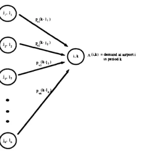
We consider a network of airports n = 1,..., N. For airport n, the aircraft arrival process is highly time-varying, especially in the case of a hub, where traffic is concentrated into banks. We suppose initially that the process is deterministic but time-varying. We divide time into short intervals of fixed length At and let the number of aircraft demanding to land at airport n in period k be given by the parameter A. Within period k these arrivals are assumed to constitute a uniform flow. Landing capacity at airport n during a given interval k is assumed to be in one of S(n) states i = 1,..., S(n) corresponding to

capacity values i1, t ,·.. ns(, ) where

1 < 2 < *** <

HS(n)-These states correspond to the capacities available under different configurations and weather conditions. In an application of our model to Dallas-Fort Worth (Peterson, Bertsimas, and Odoni 1992) , we found S(n) = 6 to be an adequate number of capacity states.

For a given capacity state i at airport n we assume a random holding time T1 which follows an arbitrary discrete distribution

P(,n) = Pr{(~7 = in},

the probability of a capacity pi period lasting for precisely m intervals of length At. Upon exiting a state i, the capacity process enters another state j y i with probability Pij. Later in the paper we shall assume holding tines to be geometrically distributed, so that the capacity process follows a Markov chain. The results of the DFW study suggest that this assumption does not strongly affect the results.

We focus for the moment on a single airport and omlit the superscript n. Within any interval k, the queue behaves like a deterministic flow process. Thus if qk is the length of the

queue at the end of some period k, then the queue length one period later is the maximum of 0 and the values qk + Ak - i for i = I .... S. We enlarge the state space to be {i, m}, where i is capacity and m the age (in intervals) of that capacity. The combined age-capacity process is Markov with transition probabilities

Pii(m) Pr ((i, m) i (i, m+ )) _{Pr Ti > m + 1 I Ti} > m. (1) We next define the following random variables:

Qk Queue length at end of interval k,

Wk - Waiting time at end of interval k,

Ck Capacity state at end of interval k,

Ak Age of current capacity state at end of interval k, Ti Random lifetime of capacity state i.

For mean queue length we introduce the notation

Qk(l, i, m, q) E Qk I Q = q, C = i, Al = m (2)

k= ,...,K, i = 1,...,S, Mn=1,...,M, < k, q = 1, . . ,qma,,(k,i),

where qmax(k, i) is the maximum attainable queue length at the end of period k, given that at that time the capacity state is i. This obeys the recursion

qmax(k, i) = qma(k- 1) + Ak - i+ (3)

where qma,,(k) = maxi qma(k, i) and x+ = max(x, 0). Similarly, for waiting times we employ the notation

Wk(l,i, in,q) = E IWk IQ, = q,CL = i, A = m]. (4) We write the second moment analogs of (2) and (4) as Q(1, i, , q) and W(1, i, m, q), respectively.

Let (x A y) denote min(x, y). The quantities Qk(l, , in, q), Q (l, i, mi, q), W (l, i, n, q),

and Wk2(1, i, m, q) can be calculated recursively, (Peterson, Bertsimas, and Odoni 1992). We repeat here the basic equations:

Qk(l, i, in,q) =

Pij(n(m)Q

+l

joi

Pii((n)Qk (+ l, i, in+ 1,

(q +

+l

Q(l, i,m, q) = EPij(7n)Q (l + l,j, I,(q + l -Ij)+) +

jsi

Wk (1, i, m, q) Wk2(1, i, m, q) Wk(k, i, mn, q) =

Pij

Pii(m)

[(-

AHi Clik(

(10)

with boundary conditions

Qk(k, ,q) - q, Q (k,,,q) q2, Wk(k, ,,0) = 0. (11) (12) (13) (14) For a single airport in isolation, equations (5) - (14) allow us to compute recursively the expectations and variances for queue lengths and waiting times at the end of each interval, based on given initial conditions. This can be achieved with computational complexity O(S2K2MQmax), where S is the number of caplacity states, K the total number of time intervals, M an upper bound on the mllemory argument rn, ald Qm, = maxk qmax(k) is the

highest attainable queue length over all periods. In the more specialized Markov case, the dimension m is unnecessary, and the runningz time re(luces to O(S2K2Qmax).

(Consider now a network of airlports = 1, 2 ... . N. On this network let there be a set A of aircraft numbered v = 1, 2 ... , V. D)ivide the operating day into periods of length At, numbered as k = 1,2,..., K. Each aircraft v has an itinerary

z(v) (i',t,s,)} in = 1,2,...,

(7)

(8)

where

·v A

m rmth stop on itinerary of aircraft v,

tM

Aircraft slack between stops m- 1 and m is the amount of time available to the aircraft at stop in - 1 beyond the minimal time necessary to turn the aircraft around. In the network schedules are no longer exogenous and deterministic, as delays at one airport affect the schedules at others. In the terminology of queuing theory, the system is a multi-class queuing network, with the classes being the different aircraft with their individual itineraries. Service capacity at each airport is an autocorrelated stochastic process described by a semi-Markov process or semi-Markov chain. Thus our task is to describe the transient behavior of a multi-class queuing network with autocorrelated service rates at each node. This high degree of complexity suggests that approximation methods are necessary.

2

A Simple Decomposition Approach

A first approximation approach is based on the following idea. Suppose that at the start of the day, one knows the schedules for all aircraft operating in the network. Under the assumption that delays are zero at the outset of the day, the schedule for the initial period of the day is fixed. Hence the first period demands are fixed, and mean queue lengths and waiting times for each airport during this period may be determined by applying equations (5) - (14) to each airport. The resulting expected waiting times for period 1 are estimates of the delay encountered by all aircraft scheduled to land in this period. Taking into account the slack which these aircraft have i their schedlules anld updating future arrival streams accordingly, one then fixes demand for the next p)eriodl calculates the resulting new expected waiting times, and so forth.

More formally, let d represent the current cumulative delay for aircraft v - i.e. as aircraft v proceeds through its itinerary. d' is the current amount by which it is behind schedule. Further define the terms

A(n, k) = set of aircraft scheduled to land at n in period k,

Ak _{k =} - number of scheduled arrivals at airport i during period k.

The arrival times t are real numbers which represent times within the integer time periods. Time t = 0 is the start of the operating day. Let ic(t) be the function which takes real time values into their corresponding periods:

t /<(t)= f

l-The scheduled arrival rates {Ak } are determined from the sets of aircraft A(n, k) which are in turn determined by the itineraries I(v):

An = IA(n,k)I (15)

A(n, k) = {v: (n, t, s) E I(v) for some s and K(t) = k} (16) Consider an aircraft which arrives at airport n at some time t during period k. A reasonable estimate of this aircraft's waiting time to land is the convex combination of expected waiting times at the end of periods k-1 and k,

aE [Wk_ ] +(1 - a)E WkJ, (17)

with the weight a determined by whether t lies closer to the end of period k or k-1:

= At

Not all of this delay is necessarily propagated to later points in the system, however, because of slack, and cumulative delay d is adjusted to reflect this fact. To illustrate, let the above aircraft's next scheduled stop (stop m+l) be n' at time t', and suppose that from the current stop until the next stop there is an available slack of s'. Prior to the mth stop, the aircraft's cumulative delay was dv; thus its new scheduled arrival time is given by

t'(d ( + aE [WL ,] + (I -a)E( WWk] -s')+.

In words, the aircraft's delay into its next stop is the maximum of zero and the value X = current delay + new congestion delay - schedule slack .

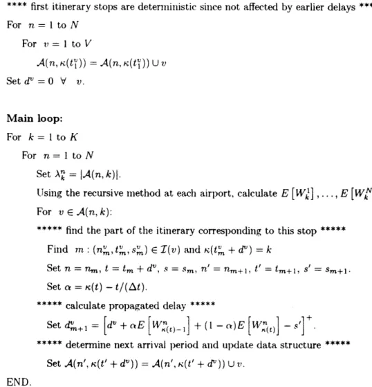
Algorithm 1, based on this simple idea, is given in Figure 1.

The algorithm consists of two main parts: complutation of expected waiting times and updating of schedules. To accomplish the former, we must aggregate aircraft and compute

First Decomposition Algorithm for Air Network Congestion

Initialize:

For k = 1 to K For n = 1 to N

A(n,k) =

**** first itinerary stops are deterministic since not affected by earlier delays ***** For n = I to N For v = 1 to V A(n, (t')) = A(n, K(tv)) U v Set d = V v. Main loop: For k = 1 to K For n = 1 to N Set A = IA(n, k)l.

Using the recursive method at each airport, calculate E [Wk] ,..., E [WkN]. For v E A(n, k):

***** find the part of the itinerary corresponding to this stop ***** Find in: (n,t, s") E (v) and (t' + d) = k

Set n = rnm, t = tm + dv, s = m, n' = n,+l, t' = tm+1, s' = sm+l.

Set a = ,K(t) - t/(At).

***** calculate propagated delay *****

Set + =+ [dv + caE [W(t)_ ] + ( I-a) E [WL] -s'] +

***** determine next arrival period and update data structure ***** Set A(n', K(t' + dV)) = A(n', K(t' + d)) U V.

END.

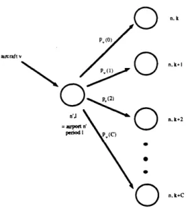
the level of demand at each airport, while in the updating procedure we must disaggregate again to the level of individual aircraft. Because of this repeated aggregation and disaggre-gation, the choice of data structures is important. For the implementation discussed here, the central data structure is the one illustrated in Figure 2. The arrival sets A(i, k) are singly linked lists of aircraft indexed by their currently scheduled destination i and arrival

Curreot Arrival Matrix

Figure 2: Data structure used in network congestion algorithms

period k. Each aircraft record contains a pointer to its schedule, another linked list, and a pointer to the current destination in that schedule. In a given period, the number of aircraft records hung from a particular location in the data structure constitutes the demand rate. This counting is the aggregation procedure. Once the resulting queuing delay is calculated for this period and location, each affected aircraft record is rehung from a new part of the arrival matrix based upon its slack and schedule. This update is the disaggregation procedure.

where U is the complexity of the single hub recursive algorithm for waiting time moments with deterministic input.

PROOF:

The choice of data structure means that the inner updating loop (the disaggregation proce-dure) requires only O(V) time. Hence the bottleneck of the algorithm consists of repeated calls to a subroutine for computing expected waiting times. Because for each time period k the algorithm must recalculate all of the preceding expected waiting times, overall

com-plexity is O(KNU). [ In Peterson, Bertsimas,

and Odoni (1992) it was shown that for a Markov model of capacity, the complexity of the recursive algorithm for a single hub is O(S2K2Qma). Thus if the Markov capacity model is specified with S capacity states, overall complexity for Algorithm I is O(NS2K3Qmax).

The presence of the additional factor K arises from the fact that the recursion at each hub is restarted from time 0 at each new period. Thus in the first global iteration the algorithm finds E[Wll]... E[WNl, in the second it finds E[W' ... E[WIN] and E1W21] ... E[W2N], and

so forth. This duplication of effort could be avoided if it were possible to store within the single hub algorithm the end conditions of iteration k as initial conditions for iteration k+1. However, even for the simpler Markov capacity model, this would mean storing the joint probabilities for queue length and capacity. Since computing these probabilities requires O(Qmax) times as much effort as for the expectation alone (see Peterson, Bertsimas, and Odoni 1992), there is no benefit to doing so unless the probabilities themselves are desired for some other reason.

A more practical improvement is to have the recursion restart only every m periods, where in is the minimum number of periods any aircraft has between scheduled stops. Under this scheme, the algorithm is run for the first n periods, arrivals are updated, then the algorithm is run for the first 2in periods, and so on. Whereas in the original implementation, the number of iterations performed within the recursive algorithm is

+2+...+ K = h'(hK+)/2, under this new scheme it is

where G = LK/7nJ and

K K if Gm< K 0 otherwise

This modification alone leads to substantial savings. The number of iterations is reduced by a factor

K(K+1)/2 > K(K+1)

rnl/mJ (LK/ mJ + 1) K (K/m + 1)

K+1 K/m+ 1.

In the case K = 80, for example, a value of mn = 10 implies that the number of iterations is reduced from 3240 to 360, one-ninth of the former number. We note that because of the higher computational requirements of the network problem, the speed advantage of the Markov model over the seni-Markov model is substantial. For this reason, our computa-tional tests in Section 4 employ the Markov formulation of capacity.

3

An Algorithm with Probabilistic Updating

The updating scheme of the previous section takes deterministic arrival streams and uses expected waiting time information to convert them into new deterministic arrival streams. A more sophisticated method would take into account the variance in the waiting times, as well as the mean, in specifying information about future arrivals rates. These arrival rates are thus specified probabilistically rather than deterministically.

Consider a particular airport n at period k, and let the expectation and variance of the waiting time at that point be denoted sinml)ly as p and a2. Suppose that it is possi-ble front these parameters to estimate an apl)lroximate density fk'(w) for the waiting time

Wk. From this density and knowledge of the schedule slacks, one can then characterize (probabilistically) the next arrival period of each aircraft v E A(n, k). More specifically, one can specify numbers p, (O),..., p, (C) and k,(O) ... , k, (C) with the following interpre-tation: the next period in which aircraft t' will land is k,(O) with probability Pv(O), k(l) with probability p,(l) and so forth. Tile user-specified p)arameter C represents an upper bound on the number of periods of delay possible. Figure 3 illustrates this phenomenon of traffic "sl)litting."

n,k

aucraft v

nn,k+I

n,k+2

) n. k+C

Figure 3: The traffic splitting phenomenon: alternative future aircraft paths depend upon delay encountered. The numbers {p,v indicate probabilities.

In order to complete the updating scheme, the algorithm must translate the probabilis-tic information on individual aircraft into infornlation on future arrival rates. Define the stochastic arrival quantities

A(n, k) = number of arrivals at airport n in period k.

The goal of this step of the procedure is to specify an approximate probability law for these random variables. For some user-specified number R (representing the number of possible values taken by the random variables) the algorithm estimates numbers k'(l1),..., 7(R) and A (1), ... , A (R) which obey the relationships

Pr{A(n,k) =A A(l)} = ~.k(1), Pr A(n. k) = A"(2)} = (2)

FPr{A(n.k)= A[.()} = R.'(R). (18)

where

Ek'(i)= 1 (19)

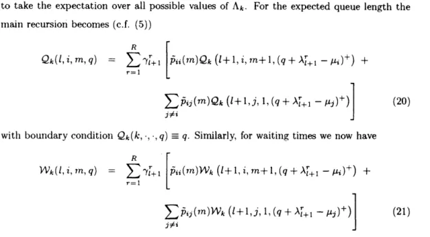
recursion for expected queue lengths. The innermost loop of the recursion is simply rewritten to take the expectation over all possible values of Ak. For the expected queue length the main recursion becomes (c.f. (5))

R

Qk(l,i,m,q) =

Zr

r=l

i(m)Qk (+l,j, 1, (q + A -j+)] (20)

with boundary condition Qk(k, , , q) = q. Similarly, for waiting times we now have

R

r= 1

k(l,i,rn,q) = ~"~ +1

[+

~

Z

Figure 3 suggests another very important point. Because of uncertainty in delays, an aircraft landing at a particular place and time takes one of many future paths. Ideally, we would like to keep track of all such future paths and thus be able to assign probabilities to all realizations of the sets A(n, k). Unfortunately, the computational complexity inherent in this task is overwhelning because of the large number of such paths - O(CC(V)) for each aircraft v, where ((v) is the number of points in v's itinerary. Thus while we can reflect the splitting phenomenon in assigning probabilities to the different values Al(.), we must limit the realizations of the sets A(n, k). To accomplish this, we repeat the method of Algorithm 1, updating each aircraft's cumulative delay by a convex combination of E[Wk] and EIWkli. Thus unlike Algorithml 1, Algorithm 2 allows a partial modeling of the splitting phenonlenon (through the AZ. 's). It should be stressed, however, that only part of the phenonlenon is captured, i.e. the immediate effect of delay uncertainty the next period's arrival rates. This splitting is not reflected when aircraft schedules are updated.

In total, the second decomposition algorithm requires four separate procedures:

1. Estimation of the densities fk (w; p(i, k), a2(i, k)) for the waiting times at each station and period, given the estimates of mean and variance computed in the recursion.

2. Translation of these density functions into probabilistic descriptions of future arrival periods for each aircraft, as given in the parameters pv (),. .. , p, v(C) and k (0), ... , kv (C). 3. Translation of the individual aircraft parameters p,(O), ... , pv(C) and k,(0), ... , k ,(C)

into simple discrete distributions for the random variables A(n, k). 4. Updating of aircraft itineraries and airport arrival lists.

The fourth of these procedures was described in Section 2. The first three are described in further detail in what follows, and a sunmmary of the algorithm is given in Figure 8.

3.1 Obtaining waiting time densities

Estimation of the densities f(w) cannot be done on the basis of the recursive algorithm alone, since this procedure gives only the first two moments of the distribution. Knowledge of the third moment would give enough information to determine a unique 2-point discrete distribution by solving the nonlinear system

Plwl + p2w2 = EJW] p12w + p2w 2 = E[W2 ]

plW +p22W2 = E [W3]

Pl +P2 = 1

P1,P2, l,W2 > 0. (22)

for the values Pt, P2, wI, and w2. However, this system is not guaranteed to have any solution because of the positivity requirement.

An alternative method is suggested by Monte Carlo methods (see e.g. Hammersley and Handscomb, 1964).. Consider a simple simlulation for a single airport in which capacity, period by period, is determined in Monte Carlo fashion from the Markov chain or semi-Markov process. From the simulation we obtain the matrix of observations

W =

{k

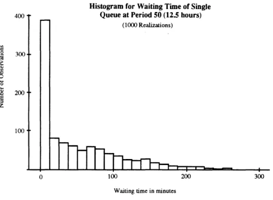
where WT is the waiting time at the end of period k for the rnth simulation. Ordering the observations, we obtain histograms for the waiting times for each period, like the one illustrated in Figure 4 for a constant arrival rate (p , 0.85, A = 60 per hour). Note the

Histogram for Waiting Time of Single 400 .* 300 .0 . 200 z 100 0 100 200 300

Waiting time in minutes

Figure 4: Histogram from simulated waiting times in a single queue

presence of a substantial probability mass at the minimum value (in this case, 0). Values above this minimum seem to follow an approximately exponential distribution. This is confirmed in Figure 5, which plots the transformations

y(m)

-where {w(m) } are the ordered values of observations which exceed the minimum and 1/ is

their mean. The fact that the graph slopes down to the right is a confirmation of the above, since according to this hypothesis the numbers exp(-iwu(n)) are realizations of the reverse cumulative distribution F(w) and thus should belhave like the reversed order statistics of a

UO10, 11 distribution. Plots suchl as this one suggest an approximate mixed distribution for the waiting times W'n:

Pr {Wk = ,min(T, k)} = 6

Pr {Wk' < w Iw > Wmin(n, k)} = I _-,(w-wi,,(nk)). (23)

The parameters Wmin (n, k), usually but not always 0, can be calculated directly from the recursion in a manner similar to that for the parameters qmax(n, k). The parameters 6 and

Exponential Plot for Positive Observations of Wait Time at Period 50 (12.5 Hours)

In _. _ , 0.8 0.6* 0.4 0.2 150 300 450 600

j = (ordered) observation number

Figure 5: Test for exponential distribution of positive waiting time realizations

v must be determined by solving the pair of equations (omlitting subscripts)

bWmin + (1 - 5) w c- (' -Wmn) dw = E[Wj

6 (Wmn)2 ( -

6)

02 - ( - Wmin)2

6 U2 (- )2 (25)

02 + (w- wmin)2

a2 ( - Win) 2

Note that is always less than 1 and will be nonnegative provided that 0.2

>1.

(' - Wmin)2

-In the typical case where Wmin is zero, this is equivalent to the condition that the coefficient

of variation for waiting tines exceeds 1. ()Only ill rare instances of the tests presented shortly was this condition found not to hold. In those cases, the parameter 6 was set to 0 and the entire distribution was assumed to be exl)onential.

3.2

From densities to schedules

Given estimated densities for W.' for all points n in the network, the next step in the procedure is to infer probabilities for the inummediate future paths of all aircraft v E A(n, k).

For any such aircraft, let (n', t', s') be the scheduled next stop (stop m+ 1) on its itinerary. The earliest period in which this aircraft's next landing may actually take place is

k,(O) = (t' + i[d + Wmin - s']+) .

This is the earliest period at which this aircraft could next land, reflecting the minimum waiting time achievable at this stop (usually 0). Accordingly, the greatest amount of delay this aircraft can endure at i and have this next arrival period remain unaltered is

w(O) = max {w' K (t' + [d + w' - s']+) = k,(O)

= {w' : t' + d + w'-s' = k,(O)At} = k,(0)At-t' - d + s'.

where d is its cumulative delay prior to the mrth stop. The probability that the aircraft's next scheduled period is kv(O) is

w(O)

Pv(O)

If Wmin = 0, which is usually the case, k(O) corresponds to the outcome that zero additional periods of delay are added to aircraft v at this stop. When the waiting time density is alpproxinlated by (23) with wmin = 0, expression (27) becomes

Pv(O) = 6 + (1 - ) 11 - exp(-Aw(O)) .

Letting w(l) = w(O) + At, the probability of the next scheduled period being k,(1)

k%(0) + 1 is

Pv(l) =

f

and in general the probability of c additiollal periods of delay is

pv(c)

-=

,

where w(c) = w(0) + cAt. These expressions take the appropriate specific fonns when the distribution (23) is substituted.

For practical reasons, it is necessary to choose some upper bound C on the number of periods of delay to allow. Hence

pv(C) =

f(w; ,a2

W

(c-l)

Together with the numbers {kv(c)}, the probabilities {pv(c)} then constitute a probabilistic description of the next period in which aircraft v will demand to land.

3.3

Characterizing arrivals

In order to translate the numbers {Pv(c)} into a probabilistic description of the future demand rates A(n, k), define the random variable

1 if v E A(n', 1) is delayed such that its

Xn',nk(V) = next stop will be n at period k

)0 otherwise

This random variable denotes the "contribution" of an arrival at one place and time to the arrival rate at a future place and time. Note that if the next stop of v E A(n', 1) is n, then

Pr{X,,,,,k(v) = 1 = p(k - ).

In words, for aircraft v E A(n', 1), the probability that it will contribute to the landing demand at airport n during period k (assuming that n is its next scheduled stop) is p(k -1). The random variables Xnql,nk(v) provide the necessary connection between aircraft and arrival rates. Then

A(n,k)

=

:

E Xn'lnk

(30)

n'=l I<k v=l

In words, this says that the arrival rate at (n, k) is the sum of all contributions from previous )oints in the itineraries (see Figure 6). Thus the random variables {A} are sums of Bernoulli random variables. [)efining

NL(v, k) next (lestillatioll of aircraft v after period k the expectation is easily obtained as

N AV

E IA(n,k)1 = E IX,,,I, E nk()l.

-n*=l 1< k v=I

E

Z

D

A (ik) = d and aLairport i

_ 1 1 in penod k

(3

0

Figure 6: Updating downstream arrivals in Algorithm 2: early arrivals and delays contribute to demands later in the day.

Obtaining the variance of A(n, k) is not straightforward because the terms of the sum are not independent. Aircraft delayed at earlier points in the day may share the same source for those delays, so that their contributions to future demands may be correlated. On the other hand, diversity in scheduling and slack weaken this dependence. For the sake of tractability, we make the approximation that the contributions are approximately independent and write

N

Var[A(n,k)I

E

S

E

n'=l <k v:NL(v,l)=n

This approximation agrees quite closely with simulation results.

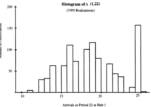
The specification of approximate distributions for the {A(n, k)} is the final step in trans-lating aircraft delays into arrival rate information. If we could compute the third moment, we could determine a 2-point distribution by solving a nonlinear system similar to (22). However, there is no easy way to obtain the third moment of A other than simulation. An alternative is to assume a normal fornl and discretize into a suitable number of points. Such a normality assumption can be partly justified on the basis of the central limit theorem, but convergence may not be good because of non-independence between terms of the sum. Simulation results indicate that for early periods of the day where there are fewer terms in the sum, unusual skewness patterns are possible (see Figure 7). These patterns disappear later in the day. While this phenomenon is cause for some concern, test runs also indicate a

200 .o 50 5O Histogram of A (1,22) (1000 Realizations) 10 15 20 25

Arrivals in Period 22 at Hub 1

Figure 7: Histogram of A(1, 22) obtained from simulation. Unusual skewness patterns such as this one may occur in the early part of the day when the contributing prior arrivals are still largely deterministic.

considerable degree of insensitivity to the demand rate distribution. We retain the normality assumption while acknowledging its imperfections.

Although Algorithm 2 involves considerably more modeling work than Algorithm 1, its computational complexity is not significantly higher, as our next result indicates.

Theorem 2 The complexity of Algorithm 2 is O(RKNUJ), where R is the user-specified

number of values used in the approximate distribution for the arrival rates and U is the complexity of the single hub recursive algorithm for waiting tzme moments with deterministic input. If the Markov capacity model is specified unith S capacity states, overall complexity is

O( RNS2K3Qm,,).

PROOF:

Within the principal loop, the bottleneck operation remains that of calculating the waiting time moments in the recursion. Because the arrival stream is specified probabilistically

Second Decomposition Algorithm for Air Network Congestion

Initialize:

For k = 1 to K For n = 1 to N

A(n, k) = , E[A(n, k)] = 0, a2[A(n, k)l = O0 For v = 1 to V

A(n, (t¥)) = A(n, K(tv)) u v

For each (n, t, s) E 1(v), EIAn(t)]= E[An(t)l + 1 Set dv = V v.

Main loop:

For k = 1 to K For n= 1 to N

From EA(n, k)] and a2[A(n, k) determine the quantities Ak(1), ,k(R) and (1),...,Yky(R)

Using the recursive algorithm with probabilistic input A, p

calculate E [W],...,E [W ] and 2(Wk ), a2(W fk) **** Update itineraries - same way as first algorithm *****

For v E A(n, k):

Find m: (nv, t ,s') E (v) and (t, + d ) = k

Set n = nm, t = tm + d, s = s, n' = iZ+l, t' = t+l, s' = sm+1.

Set a = i(t) - t/(t).

Set d = [ + aE [W(t)> + (I1 -)E ) [ Wnt)] -']

Set A(n', t(t' + dV)) = A(n', K(t' + dv)) U v. **** Update future arrival rates *****

From , EIW'I1, and o2(W7), determine the densities {fk (w)}. From the densities f(u), determine the quantities

pv(0), ... ,pv(C) and k(0) . kv(C) v E A(n,k). For c = 0 to C:

E [Ak(v,)] = E [Ak()] + P,(c)

a2

(Ak(v c)) = 2 (A(vt )) + Pv(C)( -o Pvh))

rather than deterministically, there is an additional factor R equal to the number of values specified for each arrival rate distribution. The result follows. E

Both Algorithms 1 and 2 are suitable for any kind of network. Without the streamlining suggested at the end of Section 2, running times are somewhat high. For example, onil a simple 2-airport network with K = 80 periods at each airport, Algorithm 1 takes about one hour on a DEC-3100 workstation while Algorithm 2 takes about three hours (with R= 3). With the reduction in calls to the recursion achieved by the streamlining procedure, there is roughly tenfold improvement in these figures. Even with this improvement, modeling a full-size network of a large airline (400+ nodes) is a daunting problem. On the other hand, the problem is well suited to parallel computation, with different processors handling the individual nodes and a central processor controlling the bookkeeping of aggregation and disaggregation

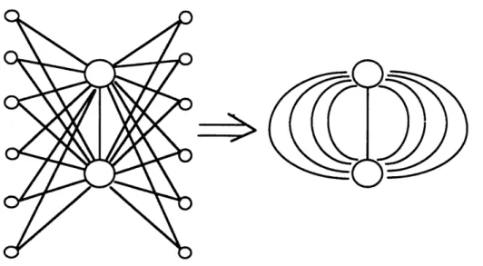
In the present context, further simplification is possible. Consider a single carrier trying to understand congestion in its own hub-and-spoke network. From this carrier's perspective, delays at its hubs have far greater implications for disruption of its schedule than delays at its spokes. This observation suggests a simnplification: reduce the hub-and-spoke network to a network of hubs. That is, keel) track only of aircraft belonging to the hub carrier, treat other arrivals as fixed, and treat all congestion delays other than those emanating from the hubs as negligible. In the resulting network, we incorporate spoke information in setting aircraft itineraries. As before, these consist of ordered triples {(i, tin, s,)}, but now each im refers to a hub airport and each s reflects the total slack available to an aircraft between successive visits to hubs, including the slack available at an intervening spoke. External aircraft add to demand and congestion in the system, but their arrival schedules are considered fixed. All internal flights in the collapsed network appear to take place between hubs, but flight timles vary widely to reflect the fact that in reality, the aircraft

have intermediate spoke stopls.

By ignloring congestion at the spokes of the system and concentrating only on the hubs, we can reduce the size of a large airline's network fromn 400+ nodes to perhaps 5 or 6. These changes reduce the model's realism, but the reduced model should capture essential behavior. Since one of the main goals is to improve our understanding of interactions between hubs (e.g. the issue of isolating C'hicago), this simlplitication seems to be further justified. The testing and analysis presented in the next section is conducted on a simple 2-hub network

'C1

Figure 9: 2-hub test network obtained from larger hub-and-spoke network

which embodies these ideas.

4

Testing the Decomposition Models

In this section we present the results of a case study conducted on a hypothetical 2-hub network, using demand and capacity data similar to those found in practice. Figure 9

illustrates the form of our test network. Following our earlier remarks, we simplify to create a network of two hubs. Each hub has two sources of demand: external demands {v' }, which are specified as parameters, and internal denlands { Ak ) which are endogenously determined according to schedules and delays.

4.1 Description of the Test Cases

Table 1 summarizes the main characteristics of nine test cases. These differ with respect to the presence or absence of banks of flights, the degree of separation between banks, the percentage p of flights which visit different hubs (rather than the same hub) on alternate visits, the traffic intensity p, the amount of slack in aircraft schedules, and the initial capacity conditions at the two hubs. The paramleter p is a lmeasure of how each hub is tied to the perfornlance of the other. In the schedules, an aircraft with an arrival at a given hub H has its next hub arrival at the other location with probability p and at H with probability

case # no. banks bank space p p slack initial capacities

1 (DFW) - 0 0.5 15-20 mrins. low/high

2a 12 15 mins. 0.5 0.9 5 mins. steady state

2b 12 15 mlins. 0.5 0.9 500 mins. steady state

3 - - 0.5 0.8 5 mins. steady state

4a 10 30 mins. 0 0.7 5 mins. low/high

4b 10 30 mins. 1 0.7 5 mins. low/high

5a 10 30 mins. 0.5 0.7 5 mnins. steady state

5b 10 30 mnins. 0.5 0.7 10 mins. steady state

5c 10 30 mins. 0.5 0.7 15 mins. steady state

5d 10 30 miins. 0.5 0.7 20 nmins. steady state

Table l: Test run information. Note that traffic intensities p are based on that part of the schedule which does not include the runout period at the end of the day. 'Steady state' indicates that initial capacities occur according to the steady state probabilities of

the Markov chain.

1 - p. A value of p = 1 implies a fully connected network (all flights alternate between the hubs), while a 0 value means a totally disconnected network.

Cases 1,2, and 3 are concerned with validation and an initial exploration of the nature of the network effects. In each case we test the models against a simulation procedure which generates period-by-period capacities at each hub using Monte Carlo methods. The simulation works in exactly the same fashion as the two approximation procedures, except that arrival rates are adjusted by simulated waiting times rather than by expected values or some approximate distribution of waiting time.

The demand and capacity data for both the hubs in case I closely resemble those at Dallas-Fort Worth. We have, however, collapsed the capacity state space to three states with steady state probabilities 0.07, 0.10, and 0.83. The simulated arrival pattern, together with the actual one for DFW, is sliown ill Figure 10. In case 1, slacks for the individual aircraft take values in the range of 1-20 millntes between stops at hubs, depending on the distance to the intervening spoke.

Case 2 provides an instance of higher traffic intensity than is present in case 1. Here internal aircraft are groupedl into identically tinted banks of 30-minutes duration at each

I DDFW demand I

Figure 10: Case 1 has demand simulated to resemble DFW.

hub with relatively short periods of 15 minutes between banks. Peak demands are higher than at DFW, capacities are slightly lower, and the underlying Markov chain has steady state probabilities 0.26,0.21,0.53 (N.B. a higher steady state probability of low capacity). The result is a considerably higher traffic intensity than in case 1 (p = 0.9 versus p = 0.5). Cases 2a and 2b differ with respect to the amount of slack in the aircraft itineraries. Case 2a represents the extreme of tight scheduling, with slack reduced to 5 minutes per stop. Case 2b, on the other hand, is an artificial case where the slack (s = 500 minutes) actually exceeds the trip time between landings. Such a situation is, of course, impossible in practice, but allowing it into the model produces an environment where delays suffered on any flight are not propagated to later parts of the day. Comparison of cases 2a and 2b thus allows us to study the effect of delay propagation o arrival schedules. Case 3 reports results for a continuous demand pattern at the two airports (no banks).

Cases 4 and 5 are concerned with the effects of slack and network connectivity on schedule reliability. Both cases have a traffic pattern like that of 2 but with lower landing demand and greater separation (30 minutes) between banks. In case 4 we illustrate the idea of hub

45 40 -35 S30 i 25 Z 20 ; 15 'S 0 5:00 7:00 9:00 11:00 13:00 15:00 17:00 19:00 21:00 23:001:00 Time of Day

isolation. by considering an instance in which the two hubs have no aircraft in common (p = 0, the disconnected case) and an instance in which they have all aircraft in common (p= 1, the fully connected case). In case 5 we examine four instances in which aircraft slack is varied.

4.2

Results and Discussion

Considering cases 1-5 together, we note that model parameters should have a noticeable effect on the mechanics of the network. For example, in the DFW case (#1), waiting times are of the same order as aircraft slack, and there is substantial separation between major. traffic peaks. For these reasons, we expect delay propagation to be relatively low and have a less disruptive effect on the schedule. In case 2, on the other hand, major peaks are much closer together, traffic intensity is sharply higher, and delay propagation should be more important.

Using a DEC-3100 workstation we performed computations for test cases 1-5, using both of our recursion-based approximations as well the the simple simulation procedure discussed above. Our investigation is primarily motivated by the desire to develop qualitative insight into the transient phenomena of the network. Accordingly, the following set of questions will guide our discussion of the results:

* To what degree do network effects alter the results obtained from the study of a single hub?

* What are the network effects produced by delay propagation and under what circum-stances do they become important?

* How closely do the network approximationl results match those of simulation? Where do they differ?

* What is the effect of congestion at one hub on dellland and congestion at the other? * How is this effect altered by the amount of slack in aircraft schedules?

* What is the effect of isolating a congeste(l hub by not allowing its flights to connect with the other hub?

Waiting Times at Hub #1 in Case #1

Figure 11: Comparison of expected waiting times predicted by one-hub algorithm, simula-tion, and the two decomposition algorithms for case 1

Network Effects in Moderate Traffic: Comparison with DFW Case Study

In our earlier paper (Peterson, Bertsinmas, and Odoni 1992), we looked at a case study of the DFW hub in isolation - that is, without taking into account delays encountered elsewhere in the network. In test case 1 (details described above), we take account of such effects.

Figure 11 plots expected waiting times at hub 1 (resembling DFW) as estimated by four different procedures: the single hub algorithm, decomposition Algorithms 1 and 2 of this paper, and simulation. There is close agreement between all four curves. The solid line indicates the predictions of the one-hub algorithm, in which all demands are treated as external and no allowance is made for propagation. The curve for Algorithm 1 (update by expected value) is quite close to this first curve, reflecting the fact that slack values (15-20 minutes) are approximately equal to expected waiting times and hence delay propagation is minimal. Algorithm 2 reflects the effects of delay p)ropagation slightly more, though the differences are still small. Finally, with the simulation curve we see a further departure from the one-hub results.

The most striking features of the graph are the closeness of the four curves and the

30 ; 25 S 20 , 20 . .9 15 X 10 5 0 0 2 4 6 8 10 12 14 16 18 20 Elapsed Hours

preservation of the peaked delay pattern, both of which indicate that the effects induced by delay propagation (the "network effects") are relatively minor. Because there is ample space between major banks and slack values are close to the mean waiting times, the general peaked pattern is preserved. The result suggests that when space between banks is adequate

to ensure a moderate traffic intensity and when mean waiting times are not substantially greater than aircraft slack, network effects are outweighed by the "deterministic" congestion effects resulting from the banked structure of arrivals at hubs.

Behavior Under Heavier Traffic and Closer Spacing

The relative weakness of the network effect in the preceding example obscures differences between the network approximations and the simulation. A more revealing picture is pro-vided by case 2a (Figure 12). Here expected waiting times (30-40 minutes) are quite high relative to aircraft slack (5 minutes), and there is only a 15-minute gap between successive banks. While the early part of the day shows a close fit between the simulation and the algorithms, there is a noticeable disparity in the middle part of the day, when alterations in the arrival stream become significant. Relative to simulation, both algorithms tend to overestimate delay during the middle part of the day, with the difference as high as 30% for

certain periods. This same effect is present in case 1 to a much lesser degree.

For a given hub and algorithm we define a standard error in the predictions relative to simulation. Let Xk denote the waiting time value predicted by algorithm for period k and Yk denote the corresponding value for the simulation. Then the standard error s is given by

_| l (Xk - Yk)2

K

This provides a measure of how far apart the simulation and algorithm results are. For Algorithm 1, these values are 4.5 and 2.6 minutes at the two hubs, while the corresponding numbers for Algorithm 2 are 4.5 and 2.3. The numbers represent an average error of 10-20%, with worse fits in the middle part of the lday.

Case 3, in which demand is allowed to be continuous over the day (no banks), also shows a discrepancy between the approxilmations and the simulation during the middle part of the day, as Figure 13 indicates. The traffic intensity for this case is higher than case 1 but lower than case 2. The difference between the algoritllhms and simulation exceeds 20% for a large part of the day at hub 2, and the standard errors are approximately 15% of the delays: 2.2

Figure 12: Comparison of expected waiting tiimles predicted by simulation and the two

decomposition methods for case 2a

minutes at hub 1 (for both algorithms) and 2.4 and 2.6 minutes (Algorithm I and Algorithm 2) at hub 2. Thus in all cases, the simulation produces lower waiting time estimates during the middle part of the day than both of the approximation algorithms. We next consider the likely explanation for the discrepancy.

The Network Effect: Demand Smoothing

Consider the waiting time profiles for cases 1 and 2a (Figures 11 and 12). Evidently, waiting time profiles are much smoother in the latter than in the former. With only a 15-minute separation between banks, the relatively high waiting times combine with low aircraft slack to overwhelm the bank structure. Thus we see that when traffic intensity is very high and aircraft slack is low, the order of the network's schedule breaks down. Further evidence of this effect is given in the top half of Figure 14, where we have plotted the original demand profiles at Hub #1 together with those which are produced as a result of delayed arrivals under scenario 2a. The original schedule is labeled "slack = 500", corresponding to the artificial situation where aircraft slack is large enough to eliminate propagation completely. We see by comparison with the situation "slack = 5" that propagated delays smooth the demand pattern substantially, with large numbers of aircraft shifted to late periods. The sharp peak structure of the original demand is considerably altered.

This smoothing phenomenon explains why Algorithms 1 and 2 overestimate delays con-sistently in the middle part of the clay. In the actual process, an aircraft scheduled at a given period may experience a delay ranging from zero up to 3 hours or more. In cases of high waiting times, the aircraft's next arrival time will be considerably later than was scheduled, and its contribution to later demand is pushed back by a significant number of periods. Thus over a large number of simulations with heavy traffic, a noticeable fraction of arrivals are pushed back to the later part of the (lay, when there is no scheduled traffic. Because capacity is more than adequate tlleli, the result of this traffic shift is to reduce overall waiting times. Ideally, the coplllutational algorithmlls should reflect this shifting and smoothing of demand. However, Its was relarked earlier, to do a thorough job they would have to keep track of the thousand.(s of lpotelltial paths which aircraft may follow as a result of delay, a seemingly impossible computatiolnal ur(ell. To linmit the state space to man-ageable size, both algorithms update aircraft schedules according to one number, expected waiting time. The result is that both algorithms tend not to shift aircraft to the very late

Figure 13: Comparison of expected waiting tilmes predicted by simulation and the two decomposition methods for case 3.

part of the day sufficiently but rather to concentrate demand more in the middle, resulting in higher predicted waits.

The Effect of Demand Smoothing on Waiting Times

The phenomenon of demand shifting and smoothing explains certain observations which seem counter-intuitive at first. An example of such a result is the fact that higher aircraft slack can. increase expected queuing times at the hubs. Cases 2a and 2b illustrate this. Both have heavy traffic organized into narrowly separated banks. The difference is that in case 2b, artificially high slack prevents the network effect of demand smoothing, whereas case 2a allows the demand to become smoother over time as aircraft are pushed back to the end of the day. In the high slack case, the higher concentration of demand produces higher queuing delays, as we see in the bottom half of Figure 14. Because slack preserves the schedule, it also preserves the peaked pattern in that schedule, which produces queues. Note that in case 2b there is a closer fit between the algorithms and the simulation, because the high slack means that the schedule becomes essentially deterministic.

Assessing the Network Approximations

The results of cases 1-3 suggest the circumstances under which network effects become im-portant, and they also indicate that under these circumstances, the network approximations developed in this paper tend to overestimate waiting times during the busy period of the day. Case 1 suggests that for networks of airports like DFW, waiting times on average are probably not high enough onl average to create siglificant network effects: the deterministic part of the schedule (i.e. the bank structure) predominates. However, as cases 2 and 3 illus-trate, the situation changes when traffic becomes heavier and spacing between major banks is decreased. This situation may only describe a few airports at present in this country (e.g. O'Hare), but it represents a future scenario which is quite possible. In the cases of heavier traffic, lower slack, and less separation, the erformance of the algorithms worsens as they tend not to capture the true spreading of demand which is the major network effect.

Slack, Connectivity, and Hub Isolation

We consider next the effect of network connectivity and aircraft slack on cumulative aircraft delay. We distinguish between this latter measure and that of the waiting times at the hubs.

rropagatea uelays Smootn uemana at rnuo Slack = 5

11CSl =

Figure 14: Top - demand rate at hub # I withll andll without the smoothing effects produced

by delays in the arrivals of incomling aircraft. Bottoli - high waiting time at hub #1

produced by unsmoothed demand.

34 30 V25 c 20 la ₀ 10 0 5 0 0 2.5 5 7.5 10 12.5 15

Elapsed Time (hours)

Unsmoothed Demand Leads to High Waiting Times at Hub #1

80 70 60 0 .40 E 30 W 20 10 0 0 2.5 5 7.5 10 12.5 15

Elapsed Time (hours)

lrl.... A J r~_1.. ~ .. L I1A .- I _~ W!__IL ~J

The latter correspond to the waiting times of aircraft at the various stations in the network, while the former is really the sum of such waiting times with aircraft slack subtracted. We measure network connectivity in terms of the percentage of flights having operations at both hubs in the network. Case 4 illustrates two opposing extremes of connectivity: a fully disconnected network (case 4a), where each hub has its own set of aircraft; and a fully connected network (case 4b), where all flights alternate between the two hubs in between visits to spokes.

Case 4a models the idea of hub isolation referred to earlier. Because the network is completely disconnected (p = 0), scheduled bank times at one hub cannot be disrupted by late arrivals from the other. In contrast, case 4b ensures that aircraft encountering delays at one hub have the maximum chance to disrupt the schedule at the second, since that is their next destination after the intervening spoke. Case 4's scenario thus allows us to explore the network effects of low capacity at a single location. To do this, in both case 4a and case 4b we take the initial state of the first hub to be 1 (lowest capacity) and that of the second hub to be 3 (highest capacity). The phenomenon of interest is the propagation of delays created at the first to the banks of the second.

Our results are summarized in Figure 15, which plots average cumulative delay per arriving aircraft. The early banks show zero delay, while later banks reflect delay carried over from previous points in the itinerary. The figure indicates a degradation in performance at hub #1 when it is isolated, as well as the corresponding benefits of isolation at hub #2. Conversely, the fully connected case benefits hub #1 at the expense of #2.

Upon further examination, these results make intuitive sense. Clearly we expect hub #2's schedule to become more reliable when it is disconnected from the disruptions produced by #1. But we also see that hub #I's schedule perfortance improves when it moves in the opposite direction - from disconnected to fully connected. Examining the situation at hub #1 more closely, we notice that the delays i the connlected case seem to lag behind the delays in the disconnected case by about 2 banks (2 hours). This is no coincidence: in the connected case, the minimum time between any aircraft's successive visits to the same hub is 4 hours (4 banks), while in the discolnected case it is only 2. Thus the schedule delays produced by the congestion at hub #1I are felt 2 hours later at that hub in the connected case, producing the 2-hour lag. However, this lag does 7not fully explain the difference in the heights of the two curves in the top half of Figure 15. In the connected case, late aircraft

Hub #1 Delays Under Different Connectivities

- ( - (N - (N - (1 - (1 - ( - (1 - ( - 1

-I - (N4 (N C; C~ - -4 v~

~A

Bank

Hub #2 Delays Under Different Connectivities

C

- (' 7 (' 7 ( - ( - ( - ( - rN 7 (' 7 -- - C

~

~

~

Bank

6

Figure 15: Average aircraft delays at two hubs under different degrees of connectivity. Note that the x-axis is in terms of banks rather than continuous time - thus 2-1 indicates the first half of the second bank, 7-2 indicates the second half of the seventh bank, etc.

60 C .s I 50 , 40 '_ ' 30 CL .2 20 @ 2 10 0 o L L 30 'I , 25 = 20 'A C I-L 15 ;I C 10 CI 5 0