A chronological probabilistic production cost model to evaluate the reliability contribution of limited energy plants

A Chronological Probabilistic Production Cost Model

to Evaluate the Reliability Contribution

of Limited Energy Plants

by

Tommy Leung

B.S. Engineering, Harvey Mudd College (2005)

Submitted to the Engineering Systems Division

in partial fulfillment of the requirements for the degree of

MASTER OF SCIENCE IN TECHNOLOGY AND POLICY

at the

MASSACHUSETTS INSTITUTE OF TECHNOLOGY

MASSACH-USETTS INSTITUTE 'OF TECHNf~OLOGYv

JUN 13 2012

LIBRARIES

ARCHIVE&

June 2012

@

Massachusetts Institute of Technology 2012. All ri

s reserved.

A u th o r .... ... ... .. . . . .V

Engine ring Systems Division

May 11, 2012

Certified by...,

..

.... ...

. . ... . . . ... ...

-Ignacii J. P6rez Arriaga

Visiting Professor, Engineering Systems Division

Thesis Supervisor

Certified by..

/

Carlos Batlle

Visiting Scholar, MIT Energy Initiative

Thesis Supervisor

,~I

(N

Accepted by.

. . ... ... ....

Joel P. Clark

Pr f

or of Materials Systems and Engineering Systems

Acting Director, Technology and Policy Program

A Chronological Probabilistic Production Cost Model

to Evaluate the Reliability Contribution

of Limited Energy Plants

by

Tommy Leung

Submitted to the Engineering Systems Division on May 11, 2012, in partial fulfillment of the

requirements for the degree of

MASTER OF SCIENCE IN TECHNOLOGY AND POLICY

Abstract

The growth of renewables in power systems has reinvigorated research and regulatory interest in reliability analysis algorithms such as the Baleriaux/Booth convolution-based probabilistic production cost (PPC) model. However, while these traditional PPC algorithms can reasonably represent thermal plant availabilities, they do not accurately represent limited energy plants because of their generic treatment of time. In particular, in systems with limited energy plants, convolution-based PPC mod-els tend to underestimate the loss-of-load probability and expected nonserved energy. This thesis illustrates the chronological challenges of the traditional convolution-based PPC, proposes a modification that improves the representation of chronological el-ements, explores the reliability contribution of LEPs using the new algorithm, and demonstrates two regulatory applications by calculating a capacity payment for an LEP and the expected-load-carrying-capability metric for any generator. To the best knowledge of the author, the introduction of multiple hydro plants with different ca-pacity constraints and the calculations for marginal probabilities, prices, and revenues to a chronological PPC model are novel.

Thesis Supervisor: Ignacio J. Prez Arriaga

Title: Visiting Professor, Engineering Systems Division

Thesis Supervisor: Carlos Batlle

Acknowledgments

"The only reason for time is so that everything doesn't happen at once."

-Albert Einstein

I humbly thank Pablo, Carlos, and Ignacio for their great mentorship, excellent ad-vice, and long hours (especially with the time difference!); Ernie and Melanie for the fantastic opportunities over the last two years; and my parents for their amazingness!

Contents

1 Introduction

1.1 A brief overview of electricity markets . . . .

1.2 Reliability in electric power systems . . . . 1.3 Limited energy plants as a reliability resource . . . . 1.4 A broader context: renewables in power systems . . . .

11 11 15 16 17

2 A new proposal for evaluating power system reliability 21

2.1 Past work: production cost models . . . . 21

2.1.1 PPC assumptions . . . . 22

2.1.2 Existing literature on chronological PPCs . . . . 24

2.2 A new chronological PPC algorithm . . . . 26

2.2.1 O verview . . . . 26

2.2.2 Step-by-step illustration . . . . 28

2.3 Calculating reliability metrics . . . . 34

2.3.1 ENSE and LOLP . . . . 34

2.3.2 Probability of at least one failure . . . . 35

2.4 Calculating costs and prices . . . . 36

2.4.1 Calculating the expected generation cost . . . . 36

2.4.2 Calculating the expected revenue for each plant . . . . 37

2.4.3 Calculating expected profits . . . . 39

2.5 Comparing reliability estimates between algorithms . . . . 39

3 Exploring LEP costs and contributions to system reliability 45

3.1 LEP dispatch methods . . . . 46

3.1.1 Peak shaving dispatch . . . . 46

3.1.2 Dual objective economic-reliability dispatch . . . . 46

3.2 R esults . . . . 48

3.2.1 R eliability . . . . 48

3.2.2 Total system cost . . . . 50

3.2.3 Thermal generation . . . . 51

3.2.4 Hydro generator revenue . . . . 52

3.3 Summary . . . .. . . . . . 57

4 Regulatory tools for reliability 59 4.1 Capacity payments . . . . 60

4.2 Calculating a generator's ELCC . . . . 62

4.3 Sum m ary . . . . 64

5 Summary & Conclusions 65

List of Figures

2-1 Chronological demand . . . . 28

2-2 The initial ILDC for hour 8 . . . . 29

2-3 Use traditional convolution to dispatch thermal plants . . . . 30

2-4 Post-thermal-dispatch ILDC for hour 8 . . . . 30

2-5 Dispatch hydro resources by convolution to cover the remaining ENSE 31 2-6 Hydro reservoir convolution . . . . 33

2-7 Final ILDC for hour 8, after dispatching all thermal and hydro plants 33 2-8 Peak-shaving operations on a load duration curve . . . . 40

2-9 Chronological tracking of reliability metrics . . . . 42

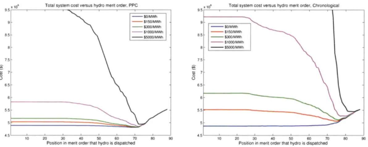
3-1 Reliability metrics for the PPC (left) and chronological (right) algorithms 49 3-2 Total system cost for the PPC (left) and chronological (right) models 50 3-3 Baseload versus intermediate-load thermal unit generation for the chrono-logical m odel . . . . 52

3-4 _{Hydro revenues for the traditional PPC (left) and chronological (right)} m odels . . . . 53

3-5 _{Hydro generation for the traditional PPC (left) and chronological (right)} m odels . . . . 54

3-6 Hydro hourly generation, chronological model . . . . 55

3-7 Hourly ENSE and hydro marginal system price, chronological model . 56 4-1 Calculating capacity payments based on ENSE, LOLP, and expected hydro revenues ... .. ... 61

List of Tables

Chapter 1

Introduction

1.1

A brief overview of electricity markets

With exception to popular historical anecdotes such as Thomas Edison's light bulb, history books today contain few electricity-related events or catastrophes. Modern so-cieties view access to low-cost and dependable electricity as a right, and until the early 1990s, vertically integrated utilities delivered reliable electricity to their consumers in a remarkably steady but otherwise unremarkable fashion.

Vertically integrated utilities

Before the early 1990s, vertically integrated utilities operated electric power networks as regulated monopolies. These monolithic entities owned all of the generation and transmission assets within their networks. They made short-term decisions about how to operate their power plants on a day-to-day basis, as well as long-term decisions about future network and generation investments. Because they operated under cost-of-service (and therefore recouped all of their investment costs), vertically integrated utilities also tended to overinvest in their network and generation assets to ensure against the physical, political, and social impacts of system failures.

Despite the greater protection that overinvestment afforded against system fail-ures, it also decreased economic efficiency and raised the average cost of electricity for consumers. To address these inefficiencies, in the early 1990s, power systems around

the world began transitioning to electricity markets. These transitions, often referred to as market "liberalization," "deregulation," or "restructuring," separated monolithic, vertically integrated utilities into four main businesses: generation, transmission, dis-tribution, and retail. Because of the economies of scale associated with transmission and distribution networks (for example, a high-capacity line loses less power than two lines that sum to the same capacity), network operations remained regulated monopolies. The most notable change for systems that liberalized occurred at the generator level with the creation of new power and reserve markets: individual gen-erators and generation companies could now compete against each other for the right to sell electricity, and new entrants could enter the market with any technology of their choosing. 1

Liberalization challenges

However, liberalization also eliminated the central planning role of the vertically integrated utility, leaving only individual agents to make both short- and long-term decisions about plant operations and investments in their own best economic interests. Although economic theory dictates that under perfect competition and information markets will drive individual agents to make economically optimal choices, in reality the individual actor (for example, an investor) does not have perfect information. Unable to forecast demand and future prices with certainty, investors in power systems with markets will likely underinvest in new power plants because they face greater

'Electricity markets, as with other markets, operate on the economic principle that perfect com-petition will produce efficient outcomes. With enough ("perfect") information about electricity prices, load trends, generation technologies, and other pertinent aspects of the power system, private enti-ties should be able to make prudent investment and operation decisions that lead to an economically efficient generation mix and electricity supply.

Concretely, in the United States, integrated system operators (ISOs) encourage competition by running auctions for the many electricity products that they need. Largely, these products are either energy- or reserve-related. Marginal prices for all products emerge from the auctions. To participate in these auctions, generators must submit bids consisting of quantity and price pairs that they are willing to sell electricity at. Additionally, because ISOs in the United States utilize complex bids, generators must also submit information about their plants' physical constraints (for example, their ramping, start-up, and shut-down capabilities). An ISO will take all bids and constraints into account to determine the economic merit order, which ranks plants from least to highest cost. Then, the ISO awards bids starting with the least expensive plants until all demand is met. In each hour, the last bid that the ISO accepts sets the marginal system price. This is the marginal system price

risks associated with recovering their costs and fewer direct consequences from failure events-directly in contradiction to the expected behavior of vertically integrated utilities.

Because private entities are free to make their own investment decisions, and be-cause they are likely to underinvest in capacity given their risk aversion, the electricity industry by and large concedes (implicitly and explicitly) that regulators still hold the responsibility for ensuring the availability of adequate capacity to prevent system fail-ures. More generally, when designing market rules, regulators have the responsibility of internalizing important political and social concerns (e.g., CO2 prices and climate

change) that consumers cannot explicitly express preferences for because electric-ity markets remain immature. As explained in [15, Rodilla 2010], most demand-side consumers have not learned how to, or cannot, respond to electricity spot prices. Con-sumers typically also do not how to, or cannot, express their preferences for products such as supply security because historically, the vertically integrated utilities man-aged these types of concerns. Although economic theory dictates that consumers, if left to market forces, would adapt and eventually learn how to express preferences for these products after enough black- and brown-outs, electricity failures impose great burdens on a society. The public at large, politicians, and governments find these failures untenable (for example, consider the Californian government's response to its 2001 blackouts) and are unlikely to allow enough time for markets to mature on their own. Consequently, because consumers are unable to directly express their preferences, regulators intervene in electricity markets to address a variety of market failures, including the problem of an inadequate security of supply.

Regulatory tools for reliability

To design market incentives and rules that guide electricity markets toward publicly desirable and economically efficient outcomes, regulators use a wide range of support tools (such as mathematical optimizations and simulations) to analyze the physical and market operations of power systems. Among the types of questions that regu-lators ask, questions about system reliability frequently surface. For example, how

reliable is a power system? What is the contribution of a particular plant to sys-tem reliability? What percentage of a plant's capacity should the regulator consider "firm?"2

With the prevalence of public subsidies for various generation technologies, questions about the intermittency challenges that renewables present, and concerns about climate change, these types of reliability questions and the tools that can be used to analyze them have once again piqued the interest of power systems researchers

and regulators.

This thesis focuses on limited energy plants (LEPs)3 as a source of system re-liability for power systems and the convolution-based probabilistic production cost (PPC) algorithms that regulators have used to evaluate the contributions of various generators (and in particular, LEPs) to reliability. Countries such as Panama, Spain, and Ireland have used PPC models in the past to determine the contribution of ther-mal and hydro generators to the reliability of their power systems. For example, in Panama, the system regulator used to calculate the reliability contribution of individ-ual generators by first, benchmarking the its entire system's loss-of-load probability (LOLP) using the PPC model; second, removing individual plants and rerunning the PPC model; and third, crediting the removed plant for reducing the probability of failure based on the net change in LOLP between the first and second steps. Although the traditional convolution-based PPC models (hereafter referred to as "traditional PPC models") that countries such as Panama have used for their reliability analy-ses can model thermal availability well, they have difficulty accurately representing limited energy plants. This thesis proposes a modification to the traditional PPC algorithm that better. addresses the representation of chronological elements. Given the recent renewed interest in regulatory instruments to encourage investments and

2

Although many definitions for "firm" capacity exist, for the purposes of this thesis, a plant's "firm" capacity refers to the fraction of its nameplate capacity that the regulator considers reliable. For example, a combined-cycle-gas-turbine plant with a nameplate capacity of 400 MW and a forced outage rate of 5% might have a firm capacity of 380 MW. Many definitions exist for firm capacity (and as many metrics for evaluating a generator's firm capacity; Chapter 4 explores one such metric). Broadly speaking, a generator that has a firm capacity close to its nameplate capacity should be more reliable than a generator with the same nameplate capacity, but a lower firm capacity.

3_{LEPs are generators that store a limited amount of energy/fuel; for instance, a reservoir-based}

behaviors that increase system reliability, the results from this thesis can make an immediate impact on discussions about the reliability contribution of LEPs and the firm capacity of various generation technologies.

1.2

Reliability in electric power systems

As noted by [14, Rodilla 2010], the physical task of delivering electricity to end consumers consists of a complex set of coordinated actions between multiple actors. At every time instant, physical laws require balance between generation and demand. Supplying electricity without interruption resembles an intricate dance between large, synchronous machines that are connected across thousands of miles and constantly converting mechanical energy into electrical energy (and vice versa). The success of this complex machine requires decisions that span multiple timescales, from building generation plants and transmission networks (processes that may take multiple years) to physically operating individual generators on a minute-by-minute and second-by-second basis. [14, Rodilla 2010] describes in detail the different temporal scales that the reliability problem can be broken down into.

For this thesis, the discussion about a power system's reliability will focus on the existence of enough installed capacity and its availability to supply demand. Within this scope, a power system's reliability can be characterized using many different met-rics. Because regulatory analyses frequently discuss reliability in terms of a system's LOLP and expected nonserved energy (ENSE), the remaining discussion about relia-bility will focus on these two metrics. Chapter 2 reviews the formal definition of LOLP and ENSE. Broadly, LOLP is the expected fraction of hours over the time period of analysis (for example, one year) in which demand will exceed available generation, and ENSE is the total expected amount of unmet demand over the time period of analysis. Using these definitions, systems with lower LOLP and ENSE values are more reliable than systems with higher LOLPs and ENSEs.

1.3

Limited energy plants as a reliability resource

Reservoir-hydro resources and storage technologies-more generally, LEPs-can con-tribute to solving the power system reliability problem. LEPs store energy in one time period for dispatch in a future time period; for this reason, LEPs face a different cost of dispatch than thermal plants. For a thermal plant, the value of generation in one hour is the difference between its operating costs and the marginal system price. For an LEP, the value of dispatching energy in one hour is the opportunity cost of not saving that energy for use in a future hour. Deciding how to best dispatch LEP resources requires a careful treatment of uncertainties that affect thermal plants to a significantly lesser degree.

Thesis objectives

Using reservoir-hydro (hereafter referred to as hydro) plants as proxies for LEPs, this thesis examines the PPC algorithms that researchers and regulators have used to evaluate system reliability. In the past, regulators have used PPCs to analyze system reliability and the reliability contributions of individual plants because PPC algorithms require relatively little computational effort and can reasonably approxi-mate thermal availability. However, these evaluations do not hold as well for LEPs. Because of their treatment of time, traditional PPCs assume one dispatch behavior for LEPs for a unit time and then scale this behavior up for the entire simulation period. Consequently, these models implicitly consider dispatch scenarios for LEPs that may violate their energy limits. Additionally, because of their treatment of time, traditional PPCs discard chronological information that may be particularly useful in the representation of certain types of LEP plants; e.g., hydro resources. To overcome these two limitations while also preserving the advantages of the convolution-based methodology, this thesis develops a chronological PPC model that can more accu-rately represent LEPs. To the best knowledge of the author, the representation of multiple hydro plants with capacity constraints and the calculation of hourly marginal probabilities, prices, and revenues in the chronological algorithm are novel

contribu-tions.

In addition to presenting the proposed chronological algorithm, Chapter 2 exam-ines how key reliability metrics are computed in both the traditional PPC and the proposed chronological model. The last section in Chapter 2 illustrates differences between the two models by applying them to a real-size case study power system. The results highlight the optimistic nature of traditional PPC models in their treatment of hydro dispatch and reliability estimates. Chapter 3 explores in depth the calculation of total system costs, marginal prices, revenues, and reliability metrics under the new chronological PPC algorithm. Chapter 4 discusses regulatory issues related to the reliability problem by applying the chronological algorithm to (1) design incentives for LEPs to improve system reliability and (2) calculate the reliability contribution of an individual generator. Chapter 5 concludes with suggestions for future research.

1.4

A broader context: renewables in power systems

Academically, the representation of chronology in PPC algorithms poses an interest-ing challenge because the trade-offs between computational effort and model accuracy impose real constraints that might have clever-yet-undiscovered workarounds. More practically, for regulatory and policy purposes, the recent growth in renewable gener-ation technologies also motivates the study of chronological PPC algorithms because LEPs can help power systems integrate larger fractions of renewables into their gen-eration mixes. The remainder of this chapter offers background about the challenges of integrating renewables to explain the greater motivation behind studying and de-veloping new algorithms (such as the PPC models presented in this thesis) for power systems.

Although supporters often cite clean emissions and free fuels as key reasons to pro-mote the adoption of renewable technologies for electricity generation, the variability of renewable generation creates new load-balancing challenges for power systems. A generator's variability depends on the intermittency and predictability of its

gener-ation.4 The lack of predictability for highly intermittent sources of electricity, such as wind and solar generators, requires power systems to make frequent supply ad-justments over shorter timescales to balance load and supply. These frequent supply adjustments can create reliability problems and impose additional costs onto other generators in the system. For example, in power systems that allow renewables to dis-patch first in violation of the economic merit order, the nonrenewable plants hold the responsibility for balancing generation and demand. Yet, the intermittency of renew-ables often increases the difference between a system's minimum and maximum net load5. Consequently, to accommodate excess wind generation on a low demand night in the spring, a coal plant might have to ramp or shut down. Ramping and cycling operations are generally uneconomic because plants incur more physical wear than usual (but are only paid for their generation), operate under decreased efficiency (con-sume more fuel per unit of electricity produced), and emit more greenhouse gasses. The inverse problem also exists: on hot summer days with.peak demand for elec-tricity, if the wind stops, the power system may not have enough thermal capacity to cover remaining demand. If the system does not have enough thermal capacity, who should be held responsible for the resources that are needed to maintain system reliability? These inversely correlated generation/ demand examples show how the variability of renewables and supportive policies such as priority dispatch can cre-ate short-term externalities for nonrenewable generators and consumers, despite the benefits of renewable electricity.

In the long-term, public subsidies for renewables and priority dispatch rules may also discourage investment in other technologies that are needed to maintain reliable

4

"Intermittency" refers to uncontrolled changes in the output of a generating resource, and "pre-dictability" refers to the ability to estimate a resource's intermittency.[1] Wind turbines, concen-trated solar power systems, and photovoltaic solar systems all exhibit high intermittency because the amount of electricity that they generate changes with the availability of wind and sunlight. However, the intermittency of these three technologies are not equally predictable. Generally, be-cause weather forecasters can forecast cloud coverage with greater accuracy over longer periods of time than they can forecast wind, wind generation tends to be more difficult to predict than solar generation.

5

The "net load" of a power system refers to its demand after subtracting out generation from nondispatchable sources such as wind and solar generators. The "net load" is the amount of demand that dispatchable generators-typically thermal and hydro plants-must provide generation for.

power systems. As capacity from renewable technologies continues to grow in power systems, despite the greater generation variability, private investors will have fewer incentives to invest in new conventional projects (such as flexible combined-cycle-gas-turbine units) because larger renewable generation mixes reduce the amount of electricity that thermal plants can sell. Market rules such as reserve capacity pay-ments can incentivize investment in flexible generation, but ambiguity surrounds the determination of who should pay for these incentives; additionally, these new market rules may not lead to the least-cost power system for the consumer. These physical, economic, and regulatory questions represent the types of integration concerns that exist for renewables, and the tools required to analyze these problems-for example, the PPC models presented in this thesis-remain an active area of research in power systems.

Chapter 2

A new proposal for evaluating power

system reliability

As described in Chapter 1, regulators have used PPC algorithms to evaluate the reliability of power systems based on their LOLP and ENSE. This chapter briefly reviews the history of PPC algorithms, describes the challenge of properly modeling LEPs with traditional PPC models, and surveys the current body of literature on chronological PPC models that offer improved representations of LEPs. The end of this chapter contains a proposal for a new chronological PPC algorithm that divides every hour into its own reliability problem, as well as a comparison of the LOLP and

ENSE results between the proposed algorithm and a traditional PPC model.

2.1

Past work: production cost models

Historically, the simplest production cost models deterministically approximated ther-mal plant failures by representing their output levels as fractions of their maximum capacities. The forced outage rate (FOR) of a plant determined the specific fraction of its total capacity that counted as firm capacity. Under this representation, thermal plants could never fail at their FOR-reduced capacities. Deterministic models treated hydro plants as thermal plants with FORs of zero, and they set hydro output levels to perfectly consume all available water in a given simulation period. This early genre

of production models did not take into consideration the fact that when plants fail, their outputs drop to zero, leading to an underestimation of the need for generation from more expensive units. [7, Finger]

The probabilistic production cost (PPC) models that followed treated thermal plant outages more realistically. Primarily developed by

[2,

Baleriaux] and reintro-duced in English by [3, Booth], PPCs represented thermal plants using a two-state model. In the first state, the plant is available to generate electricity at its full ca-pacity with probability (1 - p). In the second state, the plant is not available to generate electricity (due to a forced outage) with probability p. By considering these two potential probabilistic states, Baleriaux/Booth created a new class of production cost models that were able to more accurately capture the effect of thermal plant outages.

In the following decades, many authors proposed iterations and refinements to the Baleriaux/Booth PPC model. Of these refinements, notably [6, Conejo] developed an approach to incorporate hydrothermal coordination. More generally, the PPC techniques proposed by Conejo for optimal charging and discharging, as well as to determine the optimal merit order position to minimize system cost, applied to all LEPs (e.g., batteries, flywheels, compressed air storage)-not only hydro plants. As regulatory tools, derivatives of the Baleriaux/Booth PPC model have remained useful because they require relatively little computational effort, capture the discrete nature of plant failures, and directly convey a system's reliability in terms of its ENSE and LOLP metrics.

2.1.1

PPC assumptions

Despite the many advantages of traditional PPC models, their abstraction of time results in less accurate representations of power system. Most traditional PPC mod-els represent demand over the time period of interest, T, with a single cumulative probability distribution function (CDF). Every small t in time period T looks iden-tical. As such, traditional PPCs calculate results for one generic unit of time and

thermal plants because the dominant characteristics of a thermal plant are its capac-ity and failure rate. These characteristics do not change much with time. However, the extrapolation does not hold for LEPs because an LEP's energy constraint (how much energy it has stored) changes through time and affects its dispatch actions. Traditional PPCs unrealistically assume that an LEP's dispatch will remain constant through the simulation period T because they cannot capture how variables change with t. (A graphical explanation of this follows in section 2.2.2.)

Additionally, traditional PPC models also discard chronological information. As an example of the importance of chronology, consider hydro plants. In traditional PPC models, hydro energy targets are only enforced on the average because every t is identical in the simulation period T. If a hydro plant has 100 MWh of energy, the PPC will perfectly place every drop of water to use up all 100 MWh over time period T. However, in reality, due to inherent demand and plant availability uncertainty, in some hours hydro plants will generate less than what they should (and in others, more than they should). In the hours when hydro generation is short of the optimum, thermal plants will make up the difference. Conversely, in the hours when hydro generation exceeds the optimum, hydro operators will sell electricity that they could saved for more expensive hours. Both of these scenarios result in higher actual total system costs than those predicted by traditional PPC models because of the loss of chronological information.

As noted by [11, Maceira & Pereira 1996], chronology has not always posed a problem for PPCs. Specifically, in a thermal-dominated power system, PPC models can reasonably approximate the behavior of thermal plants. However, as the number of LEPs in a power system increases, the system's total energy constraints from LEPs take on greater importance and the assumption of a predominately thermal system breaks down. In nonthermal-dominated systems, chronological elements can cause material deviations between a PPC models' predictions about system reliability and the actual metrics for that system.

2.1.2

Existing literature on chronological PPCs

To address the limited representation of energy constraints and the loss of chronolog-ical information in traditional PPC models, [11, Maceira & Pereira 1996] proposed an algorithm that decomposes the Baleriaux/Booth PPC into a series of chronological reliability problems. The algorithm consists of a power system with multiple thermal plants and one energy-limited hydro plant. The system always dispatches its hydro plant last. Production simulations are run for time period T chronologically, hour by hour. Random variables represent inflow, demand, thermal generation, and turbine capacity. As the simulation runs, the model can probabilistically track the initial reservoir level in each hour (storage) and the hourly outflow (demand minus thermal generation). To calculate hourly reservoir levels, the simulation convolves the hourly inflow, storage, and outflow variables. Unused water carries over to the next hour, and hourly water deficits represent ENSE. The chronological algorithm produces marginal costs and reliability metrics for ENSE and LOLP in each hour. Using these outputs, [11, Maceira & Pereira 1996] compared a traditional PPC model with their proposed chronological model and determined that the traditional PPC underestimated costs for the particular system that they analyzed (as noted in their paper, the comparison is always system-dependent).

The chronological model in [11, Maceira & Pereira 19961 refined the probabilistic treatment of LEPs in PPC models by incorporating important chronological param-eters such as inflows, outflows, and reservoir storage levels. The work in this thesis builds off these results, as well as the works of other authors that have developed chronological PPC models to analyze hydro dispatch and other time-dependent ele-ments in power systems:

9 [4, Borges 2008] uses a chronological Markov chain model to analyze stochas-tic river inflows and obtain steady state probabilities for the total available energy of a small hydro power plant. Their approach covers a timescale of months and tries to improve estimates of total available hydro energy from small hydro power plants to aid long-term capacity planning. The model

sepa-rately describes the turbine portion of a hydro plant with a two-state Markov model and produces reliability metrics for the expected amount of energy avail-able taking into consideration generator failure. Instead of explicitly treating demand, Borges presents energy-availability reliability metrics for small hy-dro power plants. These metrics include a small hyhy-dro power plant's installed energy, expected available energy, expected generated energy, capacity factor (considering only the energy source), and generation availability factor.

*

18, Gonzalez 2005] describes a water dispatch policy that optimizes economic benefit, taking into consideration both cost minimization and the reliability ob-jective described by [13, Nabona 1995]. The algorithm divides a year into equal subperiods of months and combines all hydro plants into a single, monolithic hydro plant of equivalent capacity and energy. Demand is represented by a load duration curve (LDC), and the authors assume that price and demand are directly correlated. The algorithm splits hydro usage explicitly for peak shaving and to cover thermal failures. Hydro energy used to cover thermal failures is al-ways sold in the reserve market. In scenarios that have more water than ENSE for the entire year, the algorithm decides what the best allocation of water is for each multiweek subperiod. In each subperiod, an amount of hydro energy equal to the ENSE is dispatched for reliability. Any remaining hydro energy is dispatched for peak-shaving. The simulation sets the reservoir level at the beginning and does not consider inflows.

* [9, Gonzalez 2002] describes a water dispatch policy that minimizes cost, taking into consideration the stochastic nature of inflows and outflows. The simulation breaks the total time period of a year into a series of smaller periods, such as months (the algorithm generalizes well to even shorter time periods). In each interval, the simulation considers water storage, discharge, pumping, and spillage. Excess water carries from one interval to the next. Using an LDC to represent demand, the algorithm randomly samples dispatch scenarios bounded by hydro balance and feasibility rules and evaluates each scenario based on

cost. Gonzalez saves "winning" scenarios and evaluates them by simulation to determine a mean total cost and its probability distribution.

*

[10,

Gonzalez 2000] describes a hydro dispatch procedure that convolves hy-dro generation and its unavailability distribution with the LDC to capture the stochastic elements of hydro generation, based on (Nabona 1995). The simula-tion time period is one year, subdivided into months. Optimal dispatch values are found for each subperiod.

* [13, Nabona 1995] proposes a method for optimizing long-term hydrothermal usage by splitting the amount of hydro available to serve the deterministic (economic) goal of peak shaving the LDC and the stochastic (reliability) goal of covering thermal failures.

2.2

A new chronological PPC algorithm

2.2.1

Overview

To capture the chronological information that PPCs discard when they create a single aggregate LDC for all of time period T, the proposed chronological algorithm decon-structs each hour in T into its own reliability problem. To the best knowledge of the author, the introduction of multiple hydro plants with different capacity constraints and the calculations for marginal probabilities, prices, and revenues to a chronological PPC model are novel.

Thermal dispatch

In each hour, the algorithm represents demand as a discrete CDF and dispatches generation plants by convolution. For every thermal plant, the algorithm performs a single convolution between two demand CDFs. The first CDF represents demand if the thermal plant fails (i.e., the demand CDF remains unchanged). The second CDF represents demand after removing a portion of demand equal to the capacity

of the thermal plant. The FOR of the thermal plant determines the weight for each CDF (the plant fails with probability p; the plant works with probability 1 - p).

Thermal plant dispatch in this chronological PPC model closely resembles thermal plant dispatch in the traditional PPC.

Hydro dispatch

Hydro plant dispatch also largely resembles thermal dispatch, with the key distinc-tion that this algorithm also tracks the energy CDF for each hydro reservoir. In each hour that the algorithm dispatches a hydro plant, it performs two convolutions. The first convolution modifies the demand CDF, much like the thermal convolution de-scribed above. In place of thermal FORs, these demand convolutions substitute the y-intercept of the hydro reservoir CDF (representing the probability that the reservoir is empty). The y-intercept of the hydro reservoir CDF is analogous to the FOR of a thermal plant. The FOR of a hydro plant changes with time, based on the amount of energy stored in the reservoir-the more energy, the more reliable the hydro plant. The second convolution modifies the hydro reservoir CDF to reflect the amount of water released in each hour. In the hydro reservoir convolution, the scenario that hydro is needed is convolved with the scenario that hydro is not needed. If hydro is not needed, the reservoir CDF remains unchanged. If hydro is needed, then the algorithm removes an amount of energy equal to the capacity limit of the hydro plant. The intermediate LOLP values for demand determine the weights for each scenario (i.e., the probability that ENSE is strictly positive and that the system requires water is the current LOLP; the probability that ENSE is zero and that the system does not require water is the complement of the current LOLP). Modeling hydro reservoirs in this fashion allows the algorithm to uniquely distinguish water usage and availability between hours.

Lastly, the algorithm dispatches hydro plants from least to greatest capacity for maximum system reliability. Sorting hydro plants by their capacity limits acknowl-edges the fact that aside from energy limitations, large-capacity hydro plants can supply energy in all of the situations that small-capacity hydro plants can; the

re-verse is not true. (Although the energy constraint is not unimportant, it falls outside the scope of this paper). As hydro reservoirs run low on water, their availability/be-havior resembles the beavailability/be-havior of thermal plants because ENSE from previous hours reduces the certainty of water availability (i.e., increases the hydro plant's FOR) for future hours.

2.2.2

Step-by-step illustration

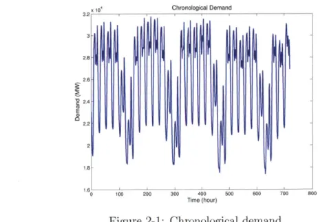
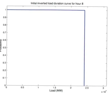
The following section graphically explains the proposed chronological algorithm. First, create an initial inverted load duration curve (ILDC) that describes a sin-gle hour of demand with absolute certainty by taking the LDC for a specific hour, inverting the x- and y-axis, and dividing the time axis by T. The ILDC resembles a CDF1 and takes on two probabilities: all demand values less than or equal to the demand at time t have probability 1, and all other demand values have probability 0. Without any loss of generality, this step can incorporate demand uncertainty by modifying the cumulative distribution probabilities attached to each discrete demand value. Figure 2-1 shows the chronological demand for this example, and Figure 2-2

shows the initial ILDC.

3 10,Chronological Demand 2.8 2.6-Fge- 2.4C E 2.2 1.8-1.6 1 _ ' Q 100 2.00 300 400 5.00 600 700 800 Time (hour)

Figure 2-1: Chronological demand

Initial inverted load duration curve for hour 8 0.9- 0.8-

0.7-

~.0.6-- 0.5-a. 0.4-0.3 -0.2 0.1 -01 0 0.5 1 1.5 2 2.5 3 Load (MW) X 10

Figure 2-2: The initial ILDC for hour 8

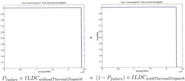
After creating the ILDC, the algorithm dispatches thermal plants using the same convolution as traditional PPCs. As described in the overview above, for each thermal plant, the convolution combines demand CDFs with and without thermal generation after weighting each CDF using the FOR (and the FOR's complement) of the thermal plant. To create the demand CDF with thermal generation, the algorithm removes an amount of demand equal to the capacity limit of the current thermal plant. Figure 2-3 shows an example thermal convolution.

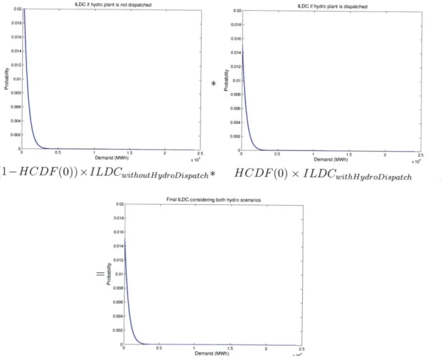
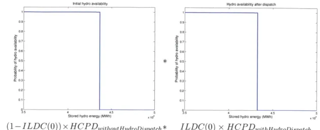
Dispatching a hydro generator resembles dispatching a thermal generator, but requires two convolutions: one for the ILDC and one for the hydro reservoir. This step describes the hydro analogue to the thermal convolution shown in Figures 2-3 and 2-4. The y-intercept of the hydro reservoir CDF, HCDF(O), represents the probability that the reservoir has water and functions much like a thermal plant's FOR. (1 - HCDF(O)) represents the probability that the reservoir is empty. Figure 2-5 shows a sample ILDC convolution for hydro dispatch.

Updating the hydro reservoir CDF (HCDFs) completes the hydro dispatch step. HCDFs are CDF-like functions that describe P(w > W), where w represents a specific amount of hydro energy. In every hour, a hydro plant faces two scenarios: either its water is needed or not. If there is no ENSE after the thermal dispatch step, then the

Hour 8, lhermal plant #1: ILDC with thermal dispatch 0.9 - 0.8- 0.70.6 -$ 0.5 -04 - 0.3- 0.20.1 -0 0.5 1 1.5 2 2.5 0 05 1 1.5 2 2.5

Demnd (MOh) 110 Demand (MWh) 1 104

Pfailure x ILDCwithoutrhermalDispatch

0 0

0

* (I - Pfailure) x ILDCwithThermalDispatch

Hour 8, thermal plant #1: post-cnvolution ILDC

.9- .6-.4 .3 - 2-.1 0 05 1 1.5 2 2.

ILDC after performing one thermal plant convolution Figure 2-3: Use traditional convolution to dispatch thermal plants

Hour 8 ILDC after dispatching thermal plants

CO -0

Load (MW) x 10

Figure 2-4: Post-thermal-dispatch ILDC for hour 8

0.9 0.8 0.7 0.6 0.5 0.4 0.2 0.1

Hour 8, thermal plant #1: ILDC without thermal dispatch

0 0

x to'

5 Load (MW)

ILDC i hydro plant is not dispatched 0.02 .018 .016 .014- .012-001 - .008.006 .004 - .002-L 0 0 5 1 1.5 2 2.5 Demand (MWh) .10, 1 - HCDF(O)) x ILDCwithoutHrydroDispatch*

ILDC it hydro plant is dispatched

0.02 .018- .016-.014 .012 .008 .006 .004 -002 0 0.5

HCDF(O)

Final ILDC considering both hydro scenarios

1 1.5 2 Demand (MWh) x x ILDCwithHydroDispatch 0.018 0.016 0.014 0.012 0.01 0.008 0006 0.002 o 05 1 1.5 Demand (MWh)

Figure 2-5: Dispatch hydro resources by convolution to cover the remaining ENSE

2.5 10 2 2.5 x 10' 0 0 0 0 0 0 0 0 0 0 0 0 0 0 0 0

0.

system does not need to dispatch any hydro generation. If ENSE is strictly positive after dispatching all thermal plants, then the hydro plant should be dispatched at the lesser of (1) its maximum capacity, or (2) the peak system demand. For most power systems, because hydro capacity is a small fraction of the peak demand and therefore also the limiting constraint, most hydro plants will be dispatched at their full capacity. The probability that water is needed is equal to the intermediate LOLP,

ILDC(O). The complement is as expected: the probability that water is not needed

is (1- ILDC(O)). The two hydro scenarios are combined by convolution to obtain the new HCDF, as in the traditional PPC approach for dispatching thermal plants. As the algorithm consecutively dispatches hydro plants within the same hour, because each hydro plant dispatch modifies the ILDC, each successive hydro plant sees a dif-ferent (and lower) intermediate LOLP. Figure 2-6 illustrates the reservoir convolution graphically. Figure 2-7 shows the final ILDC for hour 8. In each hour, hydro plants are dispatched sequentially, from lowest to highest capacity, to maximize reliability.

After completing thermal and hydro dispatch for one hour, the algorithm saves the final ENSE and LOLP values and iteratively continues onto the next hour in time period T. Because the algorithm treats every hour as its own individual relia-bility problem, this approach preserves the advantages of traditional PPCs while also addressing the chronological problem of representing all hours of demand with one generic cumulative distribution.

0 o 0 0 o o 0 0t 0 0 0 o. $0. 0. a- .

Stored hydro energy (MWh) x to'

(1

-

ILDC(O))

x HCPDwithoutHydroDispatch*

Hydro availability after dispatch 1 .98- .6-4 -3 2 -1I

Initial hydro availability

3.-5 .6 - - .4.3 - .2-3.5 4 4.5 5

ILDC(O)

x 4 4. 5

Stored hydro energy (MWh) x o

HCPDwithHydroDispatch 1 09 0.8 0.7 0.6 0.5 04 03 0.2 0.1

Hydro availability after convolution

*35 4 4.5 5

Stored hydro energy (MWh) x to

Hour 8, reservoir #1, post-convolution water availability Figure 2-6: Hydro reservoir convolution

Hour 8 ILDC after dispatching all thermal and hydro plants

0.018 -0.016 -0.014 0.012 0.01 a. 0.008- 0.006- 0.004-0.002 0-0 0.5 1 1.5 2 2.5 Load (MW) _x to'

Figure 2-7: Final ILDC for hour 8, after dispatching all thermal and hydro plants

2.3

Calculating reliability metrics

2.3.1

ENSE and LOLP

Using traditional PPC algorithms, regulators and system operators can evaluate a power system's reliability by calculating its ENSE and LOLP. ENSE represents the expected amount of nonserved energy, and LOLP represents the expected fraction of hours in T that will have a nonzero value for ENSE. The ENSE and LOLP for traditional PPC algorithms are calculated using the following equations:

m

NSEpc = E ILDC(i) (2.1) i=O

LOLPpc = ILDC(O) (2.2)

where i represents a point on the demand axis of the ILDC, and m is the peak demand of the ILDC. Given these equations, for the traditional PPC algorithm, the ENSE is the area under the ILDC curve, and the LOLP is the y-intercept of the ILDC.

For the proposed chronological algorithm, the calculations for ENSE and LOLP must take into consideration the individual ILDCs in every hour. Accordingly, the chronologically equivalent formulas are as follows:

T m NSEchrono = Z Z ILDC(i) (2.3) t=O i=O T _ILDCt(0) LO L Penrno = Et=0 T (24)

T

LOLPchrono has a normalizing term, T, that LOLPpc lacks because the PPC algo-rithm only has one ILDC for T, whereas the chronological algoalgo-rithm has an ILDC for each hour in T.

The definitions presented for ENSE and LOLP are valid for all hydro merit order positions.

2.3.2

Probability of at least one failure

Lastly, these algorithms can also produce values for the probability of having at least one hour of failure in time period T. The derivation is as follows. In each hour of the chronological dispatch model,

ILDCt(0)

is the probability of ENSE exceeding zero in that hour. The complement of this probability,

1 - ILDCt(0)

is the probability that there is no ENSE in that hour. Taking the product of these complementary probabilities for all hours in T,

T

J(1

- ILDCt(0))

t=o

gives the probability that no failures occur for time period T. The complement of this probability, Equation 2.5, is the probability that at least one failure will occur.

T

P(NSET > 0)chrono = 1 -

J(ILDCt(0))

(2.5)

t=o

The PPC equivalent simply uses the same LOLP value for every hour: T

P(NSET > O),c= 1 - 11(1 - LOLPpc) = 1 - (1 - ILDC(0))T (2.6)

t=o

The definitions presented for the probability of at least one failure are only valid for (1) completely thermal scenarios and (2) the special case of dispatching LEPs after all thermal plants. Calculating the probability of at least one failure when hydro plants are not dispatched at the end of the merit order requires determining whether a drop of water used in hour t, even if it isn't dispatched at the end of the merit order, contributes to reliability. (In turn, this step requires complicated conditional probabilities.) Dispatching hydro at the end of the merit order places an upper bound

on a system's reliability estimates.

2.4

Calculating costs and prices

In the proposed chronological algorithm, the amount of electricity that each generator produces is probabilistic. Consequently, the costs and profits (or losses) that a plant owner incurs are also probabilistic, and the comparison of costs and prices for all algorithms requires calculating expected values.

2.4.1

Calculating the expected generation cost

In every hour t, each plant p produces

m

E[generation]t,, =

Z[LDCt,p_

1

(i)

- ILDCt,p(i)] (2.7)

where (as in Equation 2.1)

i

represents a point on the demand axis of the ILDC, and

m is the peak demand of the ILDC. ILDCt,, indicates the current ILDC for hour

t after dispatching plant p; ILDCt,o represents the original ILDC for hour t. The difference on the right-hand side of Equation 2.7 is the difference of the areas under the ILDC curves, pre- and post-dispatch of plant p. Combining plant p's expected generation and variable cost, costp, gives the expected cost for plant p in hour t:

E[hourly cost]t,, = E[generation]t,, x cost, (2.8)

m

=

Z[LDCt,p_1(i)

- ILDCt,,(i)] x cost,

i=0

Summing Equation 2.8 over all hours gives the total expected cost for a single plant p in time period T:

T m

E[total plant cost) =

j[ILDCs,,_1(i)

- ILDCt,,(i)]

x

cost,

(2.9)

And, summing over all plants gives the total expected system cost:

E[total system cost]

=

E

[

[[ILDCt,,_ 1

(i)

-

ILDCt,,(i)]

x cost,

p=1 .t=1 .i=0 .

I

(2.10)

where P represents the last plant. The total expected system cost, as illustrated in Equations 2.7 through 2.10, only depends on the evolution of the ILDC after each thermal plant dispatch in every hour.

2.4.2

Calculating the expected revenue for each plant

Marginal probabilities

Calculating a plant's expected revenue requires considering the scenario that the plant is the marginal unit, as well as all of the scenarios that another plant later in the merit order is marginal. First, for a given hour t,

P(NSE is the marginal technology) = ILDC(0)t,p = LOLP (2.11)

The probability that a thermal plant is marginal is the complement of Equation 2.11:

P(any generating plant is marginal) = 1 - LOLP

Working backward, the last generating plant, P, has the following probability of being marginal:

P(the last plant, P, is marginal) = ILDC(0)t,p_1 - LOLP

More generally, the probability that any plant p is marginal in hour t is:

P(plant p is marginal in hour t) = ILDC(0),,_1 - ILDC(0)t,,

ILDC(0),0 = 1

Lastly, because either a generating plant or NSE sets the marginal price, these prob-abilities must sum to 1:

P

Z[ILDC(O)tP-I

- ILDC(),,] = 1

p=1

Marginal prices

The marginal unit probabilities calculated in Equation 2.12 represent the likelihood that plant p sets the marginal price in hour t. Each plant observes a unique marginal price because if plant p is generating electricity, then no plant beneath plant p in the merit order can set the marginal price. Therefore, the expected marginal system price in each hour for each plant p is:

E[marginal system price]t,p (2.13)

= E[marginal system price | plant p is generating]t

- [(ILDC(O),p_₁ - ILDC(O),p) x costp]

ILDC(0)t,,_1 (.4

Expected revenues

Combining the generation for each plant (Equation 2.7) and the expected marginal system price (Equation 2.13) gives the expected revenue for plant p in hour t:

E[revenue]t,, (2.15)

= _{E[marginal system price]t,, x E[generation]t,,}

- [(ILDC(O)t,_₁ - ILDC(O)t,p) x costp]

Lastly, summing across all hours gives the expected revenue for each plant:

E[total revenue], (2.16)

T

= E[revenue]t,p t=1

T ^:P [(I LDC(0)t,,_1 - ILDC(0)t,p) x costp]

E P ILDC(0),,1 'x [ILDC,,_1(i) - ILDCt,,(i)]

2.4.3

Calculating expected profits

Trivially, the difference between the revenue and cost equations (Equations 2.16 and 2.9) gives the expected profit (loss) for each plant:

E[total profit], = E[total revenue], - E[total cost], (2.17)

2.5

Comparing reliability estimates between algorithms

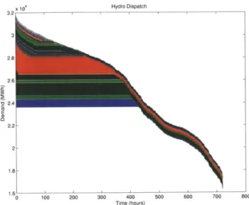
This section highlights the differences between the traditional PPC model and the proposed chronological PPC model by comparing reliability estimates from both for a case study power system. The case study power system contains 87 thermal plants, 19 hydro plants, and 720 hours of demand data. Figure 2-8 shows the system's LDC and optimal hydro coverage, assuming no thermal failures. This system has 31888 MW of thermal capacity, 9649 MW of hydro capacity, and a peak demand of 31728

MW.

For this reliability study, both the traditional and chronological PPC algorithms dispatch all thermal plants first (starting with the least expensive unit), followed by all hydro plants (starting with the lowest capacity plant). Abstracting hydro plants to LEPs, a comparison of the pre- and post-LEP dispatch reliability metrics reveals the contribution of LEPs to system reliability.

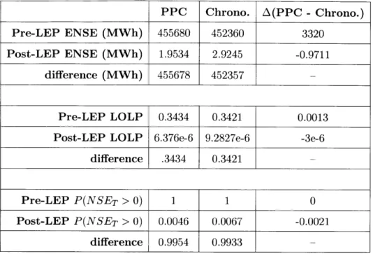
Table 2.1 contains the pre-LEP and post-LEP simulation results for ENSE, LOLP, and probability of at least one failure. Of particular and immediate interest, the estimates of ENSE and LOLP after only dispatching thermal plants differ between the

Hydro Dispatch

E

1.86

0 100 200 300 400 500 600 700 800 Time (hours)

Figure 2-8: Peak-shaving operations on a load duration curve

two algorithms. This discrepancy occurs because the initial ILDCs are not identical. The chronological algorithm contains T total ILDCs, and each ILDC initially describes demand in hour t with complete certainty. The PPC algorithm, on the other hand, contains one ILDC that initially takes on the value of the inverse demand function. The difference between each algorithm's treatment of demand and time explains why the two algorithms report different amounts of ENSE-coverage by LEPs in the system, despite the systems having identical generation plants and capacities.

PPC Chrono. A(PPC - Chrono.)

Pre-LEP ENSE (MWh) 455680 452360 3320

Post-LEP ENSE (MWh) 1.9534 2.9245 -0.9711

difference (MWh) 455678 452357

-Pre-LEP LOLP 0.3434 0.3421 0.0013 Post-LEP LOLP 6.376e-6 9.2827e-6 -3e-6

difference .3434 0.3421

-Pre-LEP P(NSET > 0) 1 1 0

Post-LEP P(NSET > 0) 0.0046 0.0067 -0.0021

difference 0.9954 0.9933

-Table 2.1: PPC versus chronological dispatch results

The post-LEP dispatch results show that the traditional PPC consistently over-estimates the power system's reliability (i.e., the traditional PPC consistently un-derestimates ENSE, LOLP, and the probability of at least one failure) compared to the chronological algorithm. The rows labeled "difference" show the amounts of ENSE, LOLP, and probability-of-at-least-one-failure reduction that can be attributed to LEP generation. Compared to the traditional PPC results, the chronological algo-rithm predicts that the LEPs will be able to cover 0.9711 MWh less ENSE, that the system has a 3e-6 greater LOLP, and that the system has a 0.21% greater chance of experiencing at least one failure for this particular month of demand. In summary, the traditional PPC simultaneously overestimates total reliability and underestimates LEP contributions to system reliability relative to the chronological PPC.

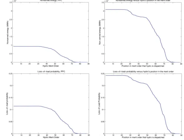
Lastly, Figure 2-9 plots the changes to ENSE, LOLP, and the probability of at least one failure as time progresses for the chronological algorithm. Because the traditional PPC algorithm treats every hour generically, equivalent graphs for the PPC algorithm would look like horizontal lines that take on the post-LEP values in Table 2.1. As expected, as time increases and the hydro reservoirs start to run out of

water, system reliability declines.

Chronological evolution of NSE when dispatching hydro for reliability

0.3 - 0,3-025 z -05 0 100 200 300 400 500 600 700 800 Time (hour)

.10- Chronological evolution of LOLP w

76 B5 -05 _j 0 100 200 300 40

hen dispatching hydro for reliability

hI

I'l ~

I

t

Time (hour)

Al

100 200 300 400 500 Tiree (hours)

Figure 2-9: Chronological tracking of reliability metrics

2.6

_{Implications for traditional PPC algorithms}

As illustrated by the traditional PPC equations for ENSE, LOLP, and probability-of-at-least-one-failure from Section 2.3, traditional PPCs treat every hour generically and then scale up results for that hour to obtain metrics for a week, month, or year. For power systems with mostly thermal units, PPCs reasonably approximate system operations because thermal availability comprises the greatest source of uncertainty, and the convolution operation adequately captures this source of uncertainty. Con-sequently, the assumption that all hours are the same in thermal-dominated power systems is valid to a first approximation. However, as shown by the results in the

pre-700 800 0

0,

they cannot distinguish one hour from the next. Because every hour in a PPC model shares the same ILDC, traditional PPC models cannot consider alternative uses for resources that have chronological dependencies. This chronological challenge reduces the usefulness of non-chronological PPC models in power systems with LEPs.