Publisher’s version / Version de l'éditeur:
Journal of Applied Polymer Science, 84, 5, pp. 1101-1105, 2002-02-15
READ THESE TERMS AND CONDITIONS CAREFULLY BEFORE USING THIS WEBSITE. https://nrc-publications.canada.ca/eng/copyright
Vous avez des questions? Nous pouvons vous aider. Pour communiquer directement avec un auteur, consultez la première page de la revue dans laquelle son article a été publié afin de trouver ses coordonnées. Si vous n’arrivez pas à les repérer, communiquez avec nous à [email protected].
Questions? Contact the NRC Publications Archive team at
[email protected]. If you wish to email the authors directly, please see the first page of the publication for their contact information.
NRC Publications Archive
Archives des publications du CNRC
This publication could be one of several versions: author’s original, accepted manuscript or the publisher’s version. / La version de cette publication peut être l’une des suivantes : la version prépublication de l’auteur, la version acceptée du manuscrit ou la version de l’éditeur.
For the publisher’s version, please access the DOI link below./ Pour consulter la version de l’éditeur, utilisez le lien DOI ci-dessous.
https://doi.org/10.1002/app.10344
Access and use of this website and the material on it are subject to the Terms and Conditions set forth at
Pressure-volume-temperature-viscosity relations in fluorinated
polymers
Utracki, L. A.
https://publications-cnrc.canada.ca/fra/droits
L’accès à ce site Web et l’utilisation de son contenu sont assujettis aux conditions présentées dans le site LISEZ CES CONDITIONS ATTENTIVEMENT AVANT D’UTILISER CE SITE WEB.
NRC Publications Record / Notice d'Archives des publications de CNRC:
https://nrc-publications.canada.ca/eng/view/object/?id=4937b1f5-19f6-4f77-baf6-26921e424a3b
https://publications-cnrc.canada.ca/fra/voir/objet/?id=4937b1f5-19f6-4f77-baf6-26921e424a3b
Pressure–Volume–Temperature–Viscosity Relations in Fluorinated Polymers
L. A. UTRACKI
National Research Council Canada, Industrial Materials Institute, 75 de Mortagne, Boucherville, Quebec, Canada, J4B 6Y4
Received 24 April 2001; accepted 8 August 2001 Published online 15 February 2002
INTRODUCTION
Recently, Mekhilef1 published new data on the
pres-sure–volume–temperature (PVT) behavior of fluori-nated polymers, polyvinylidenefluoride (PVDF), and co-polymers of poly(vinylidene-co-hexafluoropropylene) (PVDF-HFP). The author also reported on the vis-coelastic performance of these resins in the solid and molten states.
Since 1969, PVT dependencies have been analyzed by means of the Simha–Somcynsky (S–S) equation of state (EoS). The EoS has the form of coupled equations written in terms of the reduced variables:2P˜ ⫽ P/P*, V˜ ⫽ V/V*, and T˜ ⫽ T/T*. According to Rodgers’s evaluation of several EoSs, the S–S EoS has provided the best description of the PVT behavior in the whole range of independent variables.3
From the fundamental point of view, the S–S EoS has a significant advantage over other EoS relations; simultaneously with V ⫽ V(T, P), it provides the hole fraction (h) as a function of P and T: h ⫽ h(T, P). The latter function has been shown4to be directly related to
the free volume fraction ( f ), for example, as deter-mined by positron annihilation lifetime spectroscopy.5
The knowledge of h has been found useful in many applications, namely, the correlation of surface tension with bulk properties.6Furthermore, it relates the
equi-librium with transport properties, for example, the con-stant stress viscosity of melts and their mixtures7–9
and other viscoelastic functions.10
Analysis of the new PVT data for fluoropolymers is of interest for several reasons. Because the tested sam-ples were well characterized,1it would be interesting to
know how the changes of molecular weight and compo-sition affect the reducing parameters, P*, V*, and T*. Once these parameters are known, the compressibility, thermal expansion coefficient, and cohesive energy density (or the solubility parameter) can easily be cal-culated.4Furthermore, the interrelation between the
melt viscosity and h should be examined.
PVT DEPENDENCE
We fitted experimental PVT data in the molten state (kindly provided by Mekhilef) of two PVDF and three PVDF–HFP resins to the S–S EoS following the de-scribed procedure.4An example of the obtained fits is
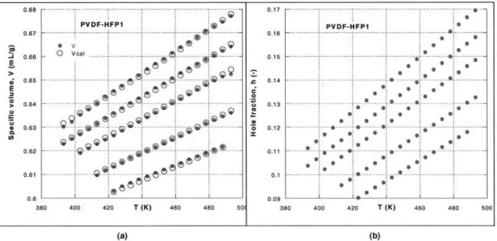
shown in Figure 1. The computed reducing parameters and the statistical measures of the fit are given in Table I.
Figure 1(a) shows the experimental data as solid points and the values computed from the S–S theory as open circles. Except for a few points at the limiting temperatures, the fit is excellent. This is also evident from the statistical evaluation of fit listed in the last three rows of Table I. The standard deviation of data ( ⫽ 0.0007– 0.0008) the correlation coefficient squared (r2⫽ 0.999998–0.999999), and the coefficient of
de-termination (CD ⫽ 0.997– 0.999) are also shown in Table I. In short, the EoS provides precise description for the observed dependencies. Figure 1(b) shows the corresponding dependence for h, h ⫽ h(P, T). Within the range of the explored independent variables, h changed from about 9 to 17%.
The resin characteristics1 {weight-average
molecu-lar weight [Mw] polydispersity factor [Mw /number-av-erage molecular weight (Mn)], and percentage of hexafluoropropylene [HFP] are also listed in Table I. The next three rows show values of the three reducing
Correspondence to: L. A. Utracki ([email protected]).
Journal of Applied Polymer Science, Vol. 84, 1101–1105 (2002) © 2002 Wiley Periodicals, Inc.
DOI 10.1002/app.10344
parameters: P*, V*, and T*, each with its own statis-tical deviation. Next, the molecular weight of the sta-tistical segment (M0⫽ RT*/3P*V*) is given. The
mo-lecular weight of the monomers are vinylidene fluoride (VDF) ⫽ 64.04 and HFP ⫽ 150.02. Hence, the statisti-cal segment that occupies a single lattice cell corre-sponds to a single VDF mer.
Rodgers11computed for PVDF (M
w⫽ 100, Mw/Mn ⫽ 2.38 at T ⫽ 178–248°C and P ⫽ 0–2000 bar) P* ⫽ 9022, V* ⫽ 0.5964, and T* ⫽ 10,440, with the average deviation of data ⌬V ⫽ 0.00091. The new computational procedure4,8,9 gave similar values: P* ⫽ 8946 ⫾ 169 bar, V* ⫽ 0.5959 ⫾ 0.0019 (mL/g), and T* ⫽ 10,360 ⫾ 92 (K). When these parameters were compared with those listed in Table I, the
differ-ences extended beyond the statistical error of the mea-surements. Thus, the PVT behavior, even of supposedly the same PVDF resin, seemed to differ. Evidently, the difference may have originated in the experimental methods and data treatment but also in the resin mo-lecular weight, composition (either by copolymerization or incorporation of additives), and chain configuration.
MELT FLOW
The dynamic data for the five resins were measured at 230°C. In the past,7it was shown that zero-shear
vis-cosity (0) or constant-stress viscosity () measured at
Figure 1 (a) PVDF–HFP1 at (from top) P ⫽ 1, 200, 400, 800, and 1200 bar. The points are experimental; the circles around them were computed from the S–S EoS fit. (b) h at P ⫽ 1–1200 bar versus T, corresponding to V versus T dependence.
Table I Summary of the PVT Data
Property PVDF1 PVDF2 PVDF-HFP1 PVDF-HFP2 PVDF-HFP3 Mw (kg/mol) 197 339 321 471 480 Mw/Mn 2.0 2.6 2.9 3.3 3.3 HFP (%) 0 0 10.5 11.1 3.1 P* (bar) 8,319 ⫾ 151 8,235 ⫾ 143 8,540 ⫾ 76 8,352 ⫾ 80 8,289 ⫾ 105 V* (mL/g) 0.6072 ⫾ 0.0018 0.6084 ⫾ 0.0017 0.5869 ⫾ 0.0008 0.5884 ⫾ 0.0008 0.5908 ⫾ 0.0011 T* (K) 10,878 ⫾ 105 10,946 ⫾ 102 10,359 ⫾ 44 10,603 ⫾ 49 10,472 ⫾ 64 M0(g/mol) 59.684 60.550 57.274 59.783 59.259 0.000859 0.000802 0.000681 0.000719 0.000740 r2 0.999998 0.999999 0.999999 0.999999 0.999999 CD 0.997276 0.997626 0.998617 0.998334 0.998318
different T and P could be superposed on a single master curve, plotting
ln 0,⫽ a0⫹ a1YS; YS⬅ 1/共a2⫹ h兲 (1)
where ai’s are the equation parameters that character-ize the material. For example, in the case of n-paraf-fins, a1⫽ 0.79 ⫾ 0.01 and a2⫽ 0.07.7For polymers,
a greater variation of values was observed. On many occasions, a2⫽ 0 was observed, turning eq. (1) into the
well-known Doolittle’s dependence, with h replacing his f parameter: ln 0, ⬀ 1/f.
To determine , we fitted the dynamic data to
⬘⬅ G⬙/ ⫽ 0/共1 ⫹ G⬙兲m (2)
where G⬙ is loss modulus, is the frequency, ⬘ is dynamic viscosity, and andmare equation constants. The goodness of fit can be judged from the data pre-sented in Figure 2 and the statistical fit parameters listed in Table II.
Equation (2) provides a method for interpolating the experimental values of ⬘ to constant shear stress, ex-pressed as G⬙ ⫽ constant. In principle, it also makes it possible to extrapolate the higher stress data to zero-shear, 0. However, as shown in Figure 2, only PVDF1
measurements provided enough data points to have confidence in the extrapolated value. The experimental range of common values of shear stress for all five resins is log G⬙ ⫽ 3.7–4.9.
Above the entanglement point, 0 usually follows
the dependence 0⫽ KMw
a with K and M being equa-tion constants. As shown in Figure 3, the plot of log 0
Figure 2 Dynamic viscosity versus loss modulus at T ⫽ 230°C for the five fluoropolymers. Points are exper-imental; lines were computed from eq. (2) with the parameters listed in Table II.
Table II Rheological Data for the Fluoropolymers Parameter PVDF1 PVDF2 PVDF-HFP1 PVDF-HFP2 PVDF-HFP3 0.00278 0.01446 0.02060 0.02725 0.02201 r 2 0.999999 0.999992 0.999982 0.999974 0.999983 CD 0.9998 0.9996 0.9991 0.9991 0.9994 log 0 3.1501 ⫾ 0.0019 4.9561 ⫾ 0.02321 4.7008 ⫾ 0.0306 5.5814 ⫾ 0.0819 5.6627 ⫾ 0.0769 m 1.0295 ⫾ 0.14503 2.0498 ⫾ 0.3259 1.6270 ⫾ 0.3752 2.8629 ⫾ 0.9591 2.6784 ⫾ 0.7300 Log ⫺ 4.2768 ⫾ 0.0854 ⫺ 4.0905 ⫾ 0.0768 ⫺ 3.8737 ⫾ 0.1065 ⫺ 4.2770 ⫾ 0.1497 ⫺ 4.2137 ⫾ 0.1105 h (P ⫽ 1, T ⫽ 2 3 0 ) 0.16120 0.15945 0.17542 0.16856 0.17221
versus log Mw followed the line log 0 ⫽ ⫺11.39
⫹ 6.3955 log Mw, with large scatter, r2⫽ 0.983. The calculated slope was also higher than what could be expected from a linear polymer (i.e., a ⫽ 3.4–3.5). That the increase was not due to the variation of com-position was evident when the two PVDF points were considered, a line connecting them had still a higher slope of a ⫽ 7.66. In short, the viscosity seemed to depend not only on molecular weight.
The last row of Table II lists the h values computed from the PVT data for P ⫽ 1 bar and T ⫽ 230°C. Evidently, this parameter depended on composition, molecular weight, and possible structural changes in-troduced during polymerization (the high value of the slope in Figure 3 suggests a long chain branching). Thus, it was tempting to see whether by combining the standard relation between 0and Mw with eq. (1) we could obtain a better description of the observed depen-dence:
log 0⫽ b0⫹ b1log Mw⫹ b2/共b3⫹ h兲 (3)
where bi’s are equation parameters. The results of this treatment are presented in Figure 3 in the form of large circles centered around the experimental solid points for all resins. The statistics of data fit gave ⫽ 0.0213, r2⫽ 0.999996, and CD ⫽ 0.99989. The values of the
four parameters were b0 ⫽ ⫺8.938 ⫾ 0.406, b1
⫽ 5.45 ⫾ 0.15, 104b
2 ⫽ ⫺1.59 ⫾ 0.29, and b3
⫽ ⫺0.1608 ⫾ 0.00006. Because of uncertainty in the determination of the experimental values of 0for this
application, eq. (3) should be treated as empirical. Next, eq. (2) was used to obtain constant-stress val-ues of the dynamic viscosity for the five fluoropolymers
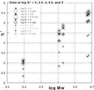
in the range of log G⬙ ⫽ 3–5. These values, along with the best fits by eq. (3) are shown in Figure 4. Evidently, the latter equation provided a good description of the observed dependencies. From between the five sets of the constant-stress data, the one for G⬙ ⫽ 104(Pa) was
the least affected by the interpolation uncertainties (see Fig. 2). The four parameters of eq. (3) were b0
⫽ ⫺10.199 ⫾ 0.146, b1⫽ 5.70 ⫾ 0.05, 104b2⫽ 2.27
⫾ 1.12, and b3⫽ ⫺0.1583 ⫾ 0.0004, with ⫽ 0.009, r2⫽ 0.999999 and CD ⫽ 99997.
DISCUSSION AND CONCLUSIONS
The S–S EoS well described the PVT behavior of the five fluoropolymers in the full range of the independent variables: P, T, and composition. As the data in Table I show, incorporation of HFP affected the reducing pa-rameters values: P* increased with HPF content, whereas V* and T* were reduced. The change in V* on incorporation of 3.1% HFP was the most dramatic. However, it seemed that in addition to the composition, these parameters were also affected by molecular weight (slightly!) and by some configurational differ-ences.
As published recently,4the S–S EoS can be
approx-imated by an analytical expression:
ln V˜ ⫽ a0⫹ a1T˜3/2⫹ P˜ 关a2⫹ 共a3⫹ a4P˜ ⫹ a5P˜2兲T˜ 2兴 (4)
where ai’s are numerical parameters. Their values are listed in the cited publication. Differentiation of eq. (4)
Figure 3 0versus molecular weight for the five
flu-oropolymers. The points represent experimental data extrapolated to zero-shear by means of eq. (2). Large circles were computed from eq. (3).
Figure 4 versus molecular weight for the five
flu-oropolymers at log G⬙ ⫽ 3–5. The points represent data interpolated to a constant value of G⬙ by means of eq. (2). Open symbols and crosses were computed from eq. (3).
readily leads to the general expressions for compress-ibility (␣) or the thermal expansion coefficient () in reduced variables, respectively:
⬅ ⫺⭸ ln V/⭸P兩T⫽ 共1/P*兲共⫺⭸ ln V˜ /⭸P˜兲兩T˜
⫽ 共1/P*兲关a2⫹ 共a3⫹ 2a4P˜ ⫹ 3a5P˜2兲T˜ 2兴
␣⬅ ⭸ ln V/⭸T兩P⫽ 共1/T*兲共⭸ ln V˜ /⭸T˜兲兩P˜
⫽ 共1/T*兲关1.5a1T˜1/2⫹ 2P˜ 共a3⫹ a4P˜ ⫹ a5P˜2兲T˜ 兴 (5)
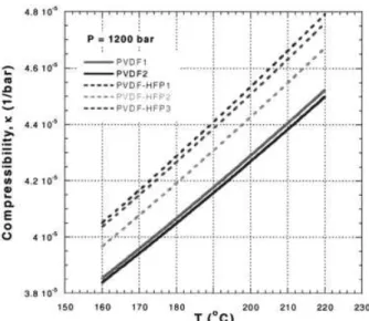
Thus, once the reducing parameters of a material are known, the  or ␣ functions in the liquid state can be calculated for any P and T. An example of  versus T dependence at 1200 bar is presented in Figure 5.
Finally, the scatter in the 0, versus Mw depen-dence vanished once the small differences in h were taken into account. Because h was affected by the mo-lecular weight, chain configuration and composition, it seems that these factors modified the thermodynamic and dynamic behavior through the free-volume contri-bution. In the past, eq. (1) has been used to account for the variation of 0,with P and T. The parameter b3
was positive, indicating that under stress, the accessi-ble free volume was larger than at the equilibrium thermodynamics. In this analysis, b3 was small and
negative, turning eq. (1) into an expression resembling the Doolittle formula.
REFERENCES
1. Mekhilef, N. J Appl Polym Sci 2001, 80, 230. 2. Simha, R.; Somcynsky, T. Macromolecules 1969, 2,
342.
3. Rodgers, P. A. J Appl Polym Sci 1993, 48, 1061. 4. Utracki, L. A.; Simha, R. Macromol Chem Phys Mol
Theory Simul 2001, 10, 17.
5. Schmidt, M. PhD Thesis, Chalmers University of Technology, Go¨teborg, Sweden, 2000.
6. Jain, R. K.; Simha, R. J Colloid Surf Sci 1999, 216, 424.
7. (a) Utracki, L. A. Polym Eng Sci 1983, 23, 446; (b) Polym Eng Sci 1985, 25, 655; (c) Can J Chem Eng, 1983, 61, 753; (d) J Rheol 1986, 30, 829.
8. Utracki, L. A.; Simha, R. J Polym Sci Part B: Polym Phys 2001, 39, 342.
9. Simha, R.; Utracki, L. A.; Garcia-Rejon, A. Compos Interfaces 2001, 8, 345.
10. (a) Curro, J. G.; Lagasse, R. R.; Simha, R. J Appl Phys 1981, 52, 5892; (b) Macromolecules, 1982, 15, 1621.
11. Rodgers, P. A. J Appl Polym Sci 1993, 50, 2075.
Figure 5 Compressibility of the five fluoropolymers computed from eq. (4). The reduced parameters from Table I were used.