Effect of cooling rate during solidification of Aluminum - chromium alloy

1

Effect of cooling rate during solidification of

Aluminum - Chromium Alloy

by

Gautham Muthusamy

Submitted to the Department of Materials Science and Engineering in partial fulfillment of the requirements for the degree of Master of Science in Materials Science and Engineering

at the

MASSACHUSETTS INSTITUTE OF TECHNOLOGY May 2020

© Massachusetts Institute of Technology 2020. All rights reserved.

Author . . . Department of Materials Science and Engineering

May 7, 2020

Certified by. . . Antoine Allanore Associate Professor of Metallurgy Thesis Supervisor

Accepted by . . . Frances M. Ross Professor of Materials Science and Engineering Chair, Departmental Committee on Graduate Studies

3

Effect of cooling rate during solidification of

Aluminum - Chromium Alloy

By

Gautham Muthusamy

Submitted to the Department of Materials Science and Engineering on May 2020

in partial fulfillment of the requirements for the degree of

Master of Science

Abstract

Controlling the distribution of alloying elements in aluminum casting and designing new processing practices are supported by an enhanced understanding of the thermodynamics and kinetics of solidification at industrial scales. While the behavior of eutectic forming elements such as copper has received a lot of attention, the interactions of peritectic-forming elements such as chromium is understudied. We herein use a time-dependent nucleation model for the calculation of the incubation time of nuclei in the liquid. This characteristic time is computed at various temperatures, and the results are presented in the form of a time-temperature diagram. Liquid phase thermodynamics of dilute compositions in the aluminum-chromium system are experimentally informed using the electrochemical potential difference method. Thermodynamic data obtained from these investigations are used to inform physical properties of the aluminum-chromium melt. The aforementioned time-temperature diagrams are recalculated using experimental data and theoretical cooling rates for phase selection are

4

calculated. Critical cooling rates calculated from the model are applied to industrially relevant practices such as DC casting and Twin roll casting.

Thesis Advisor: Antoine Allanore Title: Associate Professor of Metallurgy

6

Acknowledgments

This work would not have been possible without the help, encouragement, patience, and support of many people. The author would like to thank Prof. Antoine Allanore for his vision, support and patience. His guidance was invaluable at various points in this project. The author would like to thank Novelis Inc. for the opportunity to study an industrially relevant problem and special thanks are in order for Samuel Wagstaff, Bob Wagstaff, Barry Miller and everyone from Solatens Technology Center. The author would like to thank his amazing friends for their encouragement and friendship. The author would like to highlight the constant support from the Allanore Research Group, who helped in making this work enriching and enjoyable. Finally, the author is grateful for his family for their generosity and encouragement.

8

Contents

1.

Introduction………..…...10

1.1

Motivation……….………10

1.2

Literature Review and Background……….……….11

2. Prediction of impact of cooling rates on solidification ……….……...25

2.1

Peritectic alloy solidification interface at a microscopic scale…..25

2.2

Review of modelling attempts from Previous studies………27

2.3

Methods………28

3.

Experimental Methods……….41

3.1

Cell Materials………...42

3.2

Cell Assembly and Procedures……….44

3.3

V-shaped mold casting………..……….49

4. Experimental Results ….………...54

5. Prediction of impact of cooling rates on solidification ...67

5.1

Features of ∆t vs T diagram ………..………...68

Conclusions and Future Work……….…………80

10

Chapter 1

Introduction

1.1 Motivation

Aluminum alloys are of great importance in the light metal industry due to its low specific weight and applications ranging from aerospace, packaging and various consumer products. Almost 80 million tons of aluminum are cast every year. The ever increasing production of aluminum demands a better understanding of metallurgical properties of the cast. These properties are affected by presence of several impurity elements like Fe, Cu, Cr, Mo that are intentionally added to aluminum. Crucial properties like hardness, tensile strength and ductility are functions of morphological properties such as dendrite arm spacing and grain size distribution [1,2,3]. Controlling the distribution of alloying elements in aluminum casting and designing new processing practices are important to increase productivity. While the behavior of eutectic forming elements such as copper has received a lot of attention, the interactions of peritectic-forming elements such as chromium is understudied. For example, chromium-rich intermetallics compounds form as large needle-like particles that deteriorate mechanical properties [4]. In order to further our capability of tailoring microstructures of peritectic former with cooling rates, there is a need for additional research to investigate the possibility of suppression of the formation of the intermetallic phase at solidification. To this

11

end, a nucleation model is explored to predict microstructures of dilute Al-Cr alloys for industrially-observed cooling rates.

1.2 Literature Review and Background

Chromium is added to Al alloys, primarily to improve corrosion resistance and preventing grain growth. The following section reviews existing knowledge of the Al–Cr phase diagram [2]. This is followed by an investigation of the solidification path of dilute Al-Cr alloys and possibilities to extend solid solubility by altering this path on application of different cooling rates.

1.2.1 Thermodynamic review of Al-Cr system

The earliest work on the Al-Cr system has been dated back to 1930's [5] and subsequently multiple researchers have worked on measuring liquidus temperatures of various Al-Cr alloys. The first known phase diagram was compiled and published in 1963 by Koster [6]. Koster performed a variety of magnetic measurements and structural analysis to determine the phase diagram. Massalski [7] reported several intermetallic compounds with stoichiometries: Al13Cr2, Al11Cr2, Al4Cr, Al9Cr4 [8-12] in the aluminum rich side. The most updated version of

12

Figure 1.1: Al-Cr phase diagram reported by Okamoto [8]. It is important to note that

Okamoto refers to Al13Cr2 as Al7Cr, which have been interchangeably used in previous works.

As indicated by Figure 1.1, the solid solubility of Cr in Al is extremely limited (0.7 wt% at 661°C). Also, the phase diagram indicates that the intermetallic phases are formed by a series of peritectic reactions [13-15]. Al13Cr2 was found to be monoclinic by Ohnishi et al [13] and

later, Audier [14] reported Al11Cr2 to be orthorhombic.

In the Al-Cr system, three solution phases exist: liquid, α-Al (fcc) and β-Cr (bcc) phase. For computation of Gibbs energies, experimental data obtained from the Al-Cr phase diagram are integral. Enthalpies of formation of various phases were experimentally found by Mahdouk [16] are added as inputs, as indicated in Table 1.1.

13

Table 1.1: Enthalpies of formation and crystal structures of intermetallic compounds

The temperature of invariant reactions and the phase relationship in the Al–Cr system are also taken into account for calculation of Gibbs energy. With this data, Gibbs energies of phases were obtained by using the CALPHAD method. The solution phases (Liquid, α-Al and β-Cr) were modeled using the Redlich Kister solution model by Saunders[17]. The intermetallic phases were treated as stoichiometric compounds, which is not in accordance with the phase diagram. Liang [18] re-optimized the Al-Cr system by incorporating the fact that stoichiometric compounds have a homogeneity range. The Gibbs energy of mixing of the liquid phase predicted by both models are compared in Figure 1.3.

Phase Composition Pearson Symbol[13] Enthalpy of formation (kJ/mol) [14] At. % Cr Wt. % Cr Al13Cr2 13.3 21.4 mC104 -13.389 Al11Cr2 15.3 25.9 mP48 -15.062 Al4Cr 20 32.5 mP180 -17.15

14

Figure 1.2: Gibbs energy of mixing of Al-Cr liquid phase computed at 1100K

As evident in Figure 1.2, Liang model predicts higher excess Gibbs energies of mixing than the Saunders model in the intermediate compositions. The functional form of the Gibbs energy function are computed by minimizing an error sum by giving each piece of experimental information a certain weight. These models are very useful for preliminary analysis, but it is very difficult to capture real solution phenomena like ordering in alloy systems like Al-Cr. Therefore, CALPHAD models are challenged to accurately describe solution thermodynamics at temperatures extrapolated far from the phase boundary.

15

1.2.2 Invariant reaction in the Al-rich side of the Al-Cr system

While alloys with intermetallic compound compositions garnered attention of several researches, there is significant industry driven motivation to study the dilute composition regimes (<1 wt% Cr) of the Al-Cr phase diagram. In these dilute concentration, the solid solution of Cr in Al (referred henceforth as α(Al)) was thought to form by a peritectic reaction [15], as expressed by Eq [1].

𝐿𝑖𝑞 + 𝐴𝑙

₁₃

𝐶𝑟

₂

→ 𝛼(𝐴𝑙)

[1]

This notion was later challenged when Mahdouk [7] proposed a eutectic reaction at dilute regimes. Vilar[19] and Du[20] backed up this theory. The eutectic reaction is represented by Eq [2].

𝐿𝑖𝑞 → 𝛼(𝐴𝑙) + 𝐴𝑙

₁₃

𝐶𝑟

₂

[2]

A study of invariant reactions in the dilute regimes of phase diagram of Al binary alloys with transition metals further elucidates this conundrum, illustrated in Figure 1.3.

Figure 1.3: Binary alloys of aluminum with transition metals demonstrate change in behavior

16

Phase diagrams of Al binary alloys with transition metals demonstrate that Al–Ti and Al–V show a peritectic reaction while Al–Mn, Al–Fe, Al–Co and Al–Ni exhibit a eutectic reaction on the Al-rich side. It is interesting to note that a trend exists as we move from left to right in the periodic table. There is a clear transition from peritectic to eutectic invariant reactions as atomic number increases. It is however impossible to pinpoint whether the transition occurs at chromium or manganese. The problem is complicated by the fact that the difference in temperatures of the dilute invariant reaction (661.5°C) and melting point of pure aluminum (660.45°C) is very small [17]. In order to resolve this controversy, Kurtudlu [21] employs an innovative directional solidification study to determine the type of invariant on the Al-rich side of the Al–Cr system. He studies the Cr depletion region ahead of a quenched solid-liquid interface to prove that the invariant reaction on the Al-rich side of the Al-Cr phase diagram is peritectic.

17 1.2.2 Solidification path of dilute Al-Cr alloys

An exploded view of the Al-Cr rich part of the Al-Cr phase diagram is shown in Figure 4.

Figure 1.4: Al rich part of Al-Cr phase diagramgenerated using FACTSAGE FSlite light alloy database. The graphic on the right indicates the solidification path of a 1 wt% alloy. When Al-Cr at 1 wt% Cr alloy is cooled from liquid phase slowly, the intermetallic phase Al13Cr2 is expected to be the first phase to precipitate. On further cooling, the discussed

peritectic reaction [Eq 1] takes place to form α-(Al). It is also noted that there is a huge composition difference between the parent liquid composition (1 wt% here) and Al13Cr2 (21.4

wt% Cr as indicated in Table 1.1). This requires significant liquid phase diffusion of Cr atoms to form into Al13Cr2 clusters. With these observations, there seems to be a possibility to

kinetically limit the formation of Al13Cr2, thereby resulting in a change in the solidification path.

A fast moving solidification front caused by increasing cooling rates can restrict diffusion of Cr atoms to form Al13Cr2. This gives us a framework to investigate possibility of extending

18

solid solubility of Cr in Al by increasing cooling rates, thereby suppressing intermetallic phase nucleation.

1.2.3 Overview of casting process and possibility of solid solubility extension

To add an industrial perspective, a description of current aluminum solidification processes and cooling rates that can typically be achieved are reviewed. Direct Chill (DC) casting is the most popular method of aluminum casting on an industrial scale. Every year around 80 million tons of aluminum is casted, more than 40 million of which is produced through DC casting process [2]. The products of DC casting are billets and ingots which are rolled or forged downstream. These products have wide-ranging practical applications from cooking utensils to automobiles [22,23]. This process is a semi continuous process and a new batch starts after the casting length is reached. Cooling rates seen in DC casting are in the order of 1-20 K/s [2,24].

Another popular aluminum casting is twin roll casting is used for producing smaller cross sections like thin sheets and strips. Rolling mills can be placed adjacent to the caster, hence incorporating downstream processing. Variables like speed of rolls, heat extraction and metal feed rate are optimized. Cooling rates seen in twin belt casting are in the order of 1000K/s. Effects of cooling rate on aluminum alloys has garnered the attention of several researchers. Ichikawa[25] observed that a minimum of 120 K/s was required for extension of solid solubility in Al-Mn systems. Previous studies of solidification of binary Al-Cr alloys reveals possibility of solid solubility extension. Kobayashi[26] reported that maximum solid solubility achieved is about 6 at % in Al-Cr alloys. He made ribbons of Al-Cr alloys from rapid solidification using melt spinning technique. The extension of solid solubility has been found through lattice parameter studies. Although cooling rates of 105 _{- 10}6 _{K/s have been reported, there is no}

19

report of a direct correlation between disk speed (measured in m/s) and cooling rate (measured in K/s). Jurci[4] analyzed melt spun ribbons of Al-7 at% Cr and found a heterogeneous microstructure. V mold casts[27] can be used to analyze microstructures formed at different cooling rates. A proof of concept is presented in Section 3.3 and results are shown in Appendix A.

This following chapter explores the possibility of a theoretical prediction to achieve supersaturation in solid solution, using a dependent nucleation theory to understand phase selection at different cooling rates. Armed with the cooling rates of different casting technologies, we investigate the possibility of suppression of the formation of the intermetallic phase at solidification.

21

References

1. Kurz, W., Fischer, D.J. (1992). Fundamentals of Solidification. Trans Tech Publications.

2. Eskin DG (2008) Physical Metallurgy of Direct Chill Casting of Aluminum Alloys. Taylor & Francis

group.

3. Flemings MC (1974) Solidification Processing. McGraw-Hill.

4. Jurci P, Domankova M, Sustarsic B, Balog M (2008) Structure and properties of PM Al-7Cr alloy

prepared by rapid solidification, Powder Metall. 8(1) 217-229.

5. W.L. Fink, H.R. Freche, (1933) .Trans. AIME 104

6. W. Köster, E. Wachtel, and K. Grube. (1963). Z. Metallkd., vol. 54, p. 393.

7. T.B. Massalski, H. Okamoto, P.R. Subramanian, and L. Kacprzak. (1990). Binary Alloy Phase

Diagrams, 2nd ed., ASM Inter- national, Materials Park, OH

8. Okamoto, H. (2008). Al-Cr (Aluminum-Chromium). Journal of Phase Equilibria and Diffusion, 29(1),

112–113. https://doi.org/10.1007/s11669-007-9225-4

9. Bendersky, L. A., Roth, R. S., Ramon, J. T., & Shechtman, D. (1991). Crystallographic

characterization of some intermetallic compounds in the Al−Cr system. Metallurgical Transactions

A, 22(1), 5–10.

10. He, Z. B., Zou, B. S., & Kuo, K. H. (2006). The monoclinic Al45Cr7 revisited. Journal of Alloys and

Compounds. https://doi.org/10.1016/j.jallcom.2005.09.034

11. Ramon, J. J., Shechtman, D., & Dirnfeld, S. F. (1990). Synthesis of Al-Cr intermetallic crystals.

Scripta Metallurgica et Materiala, 24(6), 1087–1091.

https://doi.org/10.1016/0956-716X(90)90304-Y

12. Pang, M., Zhan, Y., & Du, Y. (2013). Solid state phase equilibria and intermetallic compounds of

the Al-Cr-Ho system. Journal of Solid State Chemistry. https://doi.org/10.1016/j.jssc.2012.10.020

13. T. Ohnishi, Y. Nakatani, and K. Okabayashi: Bull. (1975). Univ. Osaka Prefect, vol. 24, p. 183.

14. Audier, M., Durand-Charre, M., Laclau, E., & Klein, H. (1995). Phase equilibria in the AlCr system.

22

15. Murray, J. L. (1998). The Al-Cr (aluminum-chromium) system. Journal of Phase Equilibria, 19(4),

368–375. https://doi.org/10.1361/105497198770342102

16. Mahdouk, K., & Gachon, J. C. (2000). Thermodynamic investigation of the aluminum-chromium

system. Journal of Phase Equilibria, 21(2), 157–166.

https://doi.org/10.1361/105497100770340219

17. N. Saunders: in COST 507 Definition of Thermochemical and Thermophysical Properties to Provide

a Database for the Develop- ment of New Light Alloys, I. Ansara, A.T. Dinsdale, and M.H. Rand,

eds., vol. 2, 1998

18. Liang, Y., Guo, C., Li, C., & Du, Z. (2008). Thermodynamic modeling of the Al-Cr system. Journal

of Alloys and Compounds. https://doi.org/10.1016/j.jallcom.2007.06.046

19. Almeida, A., & Vilar, R. (2010). Al-Al7Cr eutectic in Al-Cr alloys synthesized by laser alloying.

Scripta Materialia. https://doi.org/10.1016/j.scriptamat.2010.06.022

20. Du, Y., Schuster, J. C., & Chang, Y. A. (2005). Experimental identification of the degenerated

equilibrium in extreme Al end of the Al-Cr system. Journal of Materials Science, 40(4), 1023–1025. https://doi.org/10.1007/s10853-005-6525-0

21. Kurtuldu, G., Jessner, P., & Rappaz, M. (2015). Peritectic reaction on the Al-rich side of Al-Cr

system. Journal of Alloys and Compounds. https://doi.org/10.1016/j.jallcom.2014.09.174

22. Ulam JB, McMurray PA (1987) Induction cooking utensils, US Patent 4646935, Filed on: 3rd _March

1987.

23. Frindlyander IN, Sister VG, Grushko OE, Berstenev VV, Sheveleva LM, Ivanova LA (2002)

Aluminum Alloys: Promising materials in the automotive industry. Met Sci. Heat. Treat.

44(9-10)365-370.

24. Grandfield JF, Eskin DG, Bainbridge IF (2013) Direct-Chill Casting of Light alloys. John Wiley &

Sons.

25. Ichikawa R, Ohashi T, Ikeda T (1970) Effects of Cooling Rate and Supercooling Degree on

Solidified Structures of Al-Mn, Al-Cr and AI-Zr Alloys in Rapid Solidification. Trans. JIM.

23

26. Kobayashi, K. F., Tachibana, N., & Shingu, P. H. (1989). Continuous heating of rapidly solidified

Al-Cr ribbons. Journal of Materials Science, 24(7), 2437–2443. https://doi.org/10.1007/BF01174508

27. Park, E. S., & Kim, D. H. (2005). Formation of Mg-Cu-Ni-Ag-Zn-Y-Gd bulk glassy alloy by casting

into cone-shaped copper mold in air atmosphere. Journal of Materials Research, 20(6), 1465–1469. https://doi.org/10.1557/JMR.2005.0181

25

Chapter 2

Prediction of Incubation times

We herein use a time-dependent nucleation model in order to evaluate possible impact of industrially-observed cooling rates. The predictions are obtained from the calculation of the incubation time of nuclei in the liquid. This characteristic time is computed at various temperatures, and the results are presented in the form of a time-temperature diagram. Before describing the model, a description of alloy solidification at a microscopic level is presented.

2.1 Description of alloy solidification interface at a microscopic

scale

To illustrate impact of cooling rates, assume a hypothetical dilute binary alloy with nominal composition C0 solidifying with a planar solid-liquid interface. The composition of the solid

composition Cs* can be related to the liquid composition Cl* by defining a partition coefficient

(k) [1].

𝑘 = 𝐶𝑠

∗

𝐶_𝑙∗

(2.1)

Numerical value of partition coefficient indicates the nature of solidification. For peritectic alloys, the partition coefficient is greater than unity. This indicates that slope of the liquidus of

26

the binary phase diagram is positive i.e., solute depletion at interface during solidification results in a composition profile in the liquid [2] indicated in Figure 2.1.

Figure 2.1: Solute composition profile in the liquid for a slow solidification of a peritectic

binary alloy. Vp is the velocity of the planar solidification front

The steady state composition profile shown in Figure 1 assumes that there is a finite diffusion of solute in the liquid. This indicates the ability of the solute to redistribute during solidification, as solute balance at the interface requires that there is a requirement of solute depletion at the solid-liquid interface. The liquid composition far away from the interface tends to the average composition (C0). Since such a composition profile results from diffusion of solute

atoms in the liquid, the velocity of the solidification (Vp) front should affect this redistribution.

27

Now consider solidification of the same alloy with infinitely rapidly moving solidification front (Vp -> ∞). The resultant liquid composition profile[1] is illustrated in Figure 2.2.

Figure 2.2: Solute composition profile in the liquid for a rapid solidification of a peritectic

binary alloy. Vp is the velocity of the planar solidification front

As illustrated above, diffusion limitations are kinetically suppressed by the rapid advance of the solidification front. At this point, it is important to illustrate the differences between cooling rate and solidification rate (VP). Solidification rate refers specifically to the rate of

transformation of the liquid to a solid, this solid possibly being composed of several different phases. Cooling rate refers to the rate of heat extraction measured in K/s. It is a measurable quantity that sets the driving force for phase transformation and distribution of a materials system. It is often a macroscopically controlled parameter of processing technologies, for both casting and solid-state processing. For establishing standards for comparing capabilities of casting technologies, characteristic cooling rates have been used in this study.

28

2.2 Review of modelling attempts from previous studies

Aziz [4-7] attempted to incorporate the effect of change in cooling rates on k, presenting several analytical expressions incorporating kinetic effects on partition coefficient. Aziz predicts partition coefficient accurately for a range of cooling rates for Si alloys[8]. His measurements of solute trapping during rapid alloy solidification agrees well with his predictions of partition coefficient. It is important to note that this method of studying rapid solidification is applicable for single phase systems [6,8]. Although solute trapping has been captured reasonably well, ramifications of cooling rates on solid solubility extension is not explained. Also, if several solid phases with different crystal structures can form, this model could not capture the different interfacial properties of each structures, and hence cannot be extended to systems that exhibit phase competition [6].

Alternatively, solid-state precipitation curves for different alloys have extensively been studied at different cooling rates in the context of heat treatment of aluminum alloys [9,10]. Heat treatment cycles can then be effectively designed to obtain desired shapes and distribution of precipitates. A similar study by Chinella attempts to determine cooling rates for optimal age hardening treatments for 7xxx series [11]. Taking inspiration from this, the effect of cooling rates on phase selection is herein studied by calculating the incubation time as a function of temperature difference.

2.3 Method

In this study, an analytical model is used for computing nucleation times as a function of temperature for the competing phases involved in the Al-Cr system. The biggest assumption in this model is that the solidification process is nucleation controlled. This is a common

29

assumption in systems where an intermetallic phase is present [12]. Therefore, an estimation of the time taken for the critical nucleus to form is sufficient to understand the phase selection. Nucleation rate (J) in melts has been modeled in classical nucleation studies, where the nucleation rate is expressed in Equation 2.2[13].

𝐽 = 𝐽

_𝑠

𝑒

−∆𝑡𝜏

(2.2)

Where

J

s is the steady state nucleation rate, 𝜏 is the time elapsed.

∆t

is the characteristic incubation time, which is defined as the time at which steady nucleation can start at a steady rate. Therefore for

𝜏 <

∆t

, nucleation rate (Equation 2.2) is nearly zero. The steady state nucleation rate is a function of the Zeldovich factor (Z) and Gibbs energy of a critical sized cluster (∆𝐺∗_),

𝐽_𝑠

= 𝑍𝐷

_𝑘

𝑁 exp [−

∆𝐺

∗

𝑘𝑇

]

(2.3)

Where Z is the Zeldovich factor, which gives the probability that an atom jumps from parent phase to the new phase. Dk is the defined as the frequency factor, which is the number of

atoms joining the growing cluster per second (Equation 2.4). The Zeldovich factor can be expressed as:

𝑍 = [−

1 2𝜋𝑘𝑇

[

𝜕2∆𝐺𝑛 𝜕𝑛2

]

_𝑛∗

]

1/2

_(2.3)

Where ∆𝐺_𝑛 is the Gibbs energy of nucleation, n is the number of atoms in a cluster, k is the Boltzmann constant, T is the temperature of the melt and n* is the number of atoms of a critical sized nucleus. The frequency factor is given by:

𝐷

_𝑘

=

𝐷 𝑎2

[

2𝜋𝑟2(1−𝑐𝑜𝑠 𝜃)𝑥

30

Where 𝜃 is the wetting angle, r is the radius of the nucleus, D is the diffusivity of the solute in the melt, a is the atomic jump distance and x is the composition of the melt. Several researchers have since attempted to link the incubation time (∆t) to the Zeldovich factor (Z). Kashchiev[14] approximate incubation time by considering the attachment of an atom on to the new phase as a statistical process and computes the time (∆t ) for steady state nucleation to be achieved.

∆𝑡 =

2 𝜋𝐷𝑘𝑍2

(2.5)

By substituting the Zeldovich factor, we have,

∆𝑡 = −

4𝑘𝑇 𝐷𝑘[𝜕2∆𝐺𝑛_𝜕𝑛2 ]

𝑛∗

(2.6)

To further simplify Equation 2.6, ∆𝐺_𝑛 can be expressed as,

∆𝐺

_𝑛

= 𝑃𝑛 + 𝑄𝑛

2/3

(2.7)

where, P is given by,

𝑃 =

Ω

∆𝐺

_𝑣

(2.8)

Where, Ω is the atomic volume of the liquid, ∆𝐺_𝑣 is the volumetric Gibbs energy of solidification, which is the driving force of nucleation. It is given by

∆𝐺

_𝑣

= 𝐺

_𝐿

− 𝐺

_𝑆

(2.9)

where 𝐺𝐿 and 𝐺𝑠 are the Gibbs energies of parent phase (liquid) and new phase (solid)

respectively. Now, Q in Equation 2.7 can be expressed as

𝑄 = 𝛾[36𝜋𝛺

2

𝑓(𝜃)]

1/3

(2.10)

where 𝛾 is the surface energy of the solid liquid interface. 𝑓(𝜃) is given by

31

𝑓(𝜃) =

2−3 cos 𝜃+cos3𝜃

4

(2.11)

Equation 2.6 requires the second derivative of ∆𝐺_𝑛 with respect to n to be taken at the critical sized nucleus (n*). This is related to ∆𝐺_𝑣 by the following expression

𝑛

∗

₌

4 3𝜋( 2𝛾 ∆𝐺𝑣) 3 𝛺

(2.12)

Finally, the second derivative of Gibbs energy with respect to n is given by:

[

𝜕2∆𝐺𝑛

𝜕𝑛2

]

𝑛∗

= −

𝛺2∆𝐺𝑣4

32𝜋𝛾3

(2.13)

Plugging the results obtained in Equations 2.4 and 2.13 into Equation 2.6, we have,

∆𝑡 =

16𝑘𝑓(𝜃) 1−𝑐𝑜𝑠 𝜃 𝑎4 𝛺2 𝛾𝑇 𝑥𝐷∆𝐺_𝑣2

(2.14)

The atomic jump distance in the melt was taken to 0.5nm[15]. To estimate Ώ, a linear variation of atomic volume was assumed with mole fraction. Therefore, Ώ was computed as

𝛺 = 𝑥

_𝐶𝑟

𝛺

_𝐶𝑟

+ 𝑥

_𝐴𝑙

𝛺

_𝐴𝑙

(2.15)

The individual atomic volumes are calculated by equation 2.16

𝛺

_𝑖

=

𝑊𝑖

𝑁_𝑜𝜌_𝑖

(2.16)

Where

i

refers to Cr and Al, 𝑊_𝑖 is the atomic mass, Avogadro’s number (N0) and density (𝜌_𝑖 )

32

The Gibbs energies of the liquid and the α-Al solid solution are taken from FACTSAGE FSLite light alloy Database. FSLite light alloy databases uses Saunders model (reviewed in Section 1.2) for computing mixing properties of the solution phases. These models work by approximating Gibbs energies as a polynomial function (Redlich-Kister). The coefficients of the polynomial are optimized based on available experimental information. Unfortunately, severe lack of experimental data invokes skepticism in the usefulness of thermodynamic property predictions at such compositions. For example, large negative deviations from ideality are expected in aluminum-chromium system because of the tendency to form a bunch of intermetallic compounds. These deviations originate from short range ordering exhibited in such melts, resulting in complex entropic effects which are difficult to capture with existing CALPHAD framework. Therefore, such models are extremely unreliable in estimating thermodynamic properties in dilute regimes of binary systems. Apart from this, no experimental data on the wetting properties of Al-Cr alloys and the diffusivities were found by the author. To circumvent this problem, a sensitivity analysis is performed to highlight the effect of these parameters on the incubation times. As a representative example, incubation times calculated for the 0.2 wt% Cr are presented.

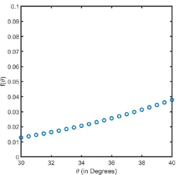
Taking inspiration from the data available in the Ti-Al system [16], four wetting angles (𝜃 = 30°, 33°, 36°, 40°) were investigated. The wetting angle impacts the incubation time in the form of 𝑓(𝜃), which is displayed in Figure 2.3. The corresponding incubation time diagram for the four cases are illustrated in Figure 2.4.

33

Figure 2.3: 𝑓(𝜃) variation with 𝜃 in the range of 30°- 40°

Figure 2.4: Incubation time vs temperature diagram of the nucleation times of Al13Cr2 phase

34

Figure 2.3 indicates that 𝑓(𝜃) does not significantly vary in the range of interest. As evidenced in Figure 2.4, the order of magnitudes of the incubation times are the same at all temperature ranges.

For sensitivity studies with respect to diffusivity, three different models were tested. The first case for diffusivity model is provided below:

𝐷 = 𝐷

₀

𝑒

−𝑄/𝑅𝑇

(2.17)

Where 𝐷₀ is the diffusivity coefficient and Q is the activation barrier for diffusion. This model is based on assuming that diffusivity had an Arrhenius dependence on temperature. The values of 𝐷₀ and Q were obtained from Du et al [17].

Case 2 was based on Stokes-Einstein model [15], which relates diffusivity to the viscosity(𝜂) of the melt. Viscosity of the melt can be computed from Equation 2.19[18].

𝐷 =

𝑘𝑇

3𝜋𝑎𝜂

(2.18)

𝜂 = 10

−3.3

𝑒

(

3.34𝑇𝐿

𝑇−0.25𝑇𝐿)

_(2.19)

Another diffusivity model worth paying attention to is the Singh-Sommer model[19], r = 0.1248 nm [20] (radius of the diffusing particle) :

𝐷

_𝐶𝑟

=

𝑘𝑇

6𝜋𝜂𝑟

𝜕 ln 𝑎_𝐶𝑟

𝜕 𝑙𝑛 𝑥_𝐶𝑟

(2.20)

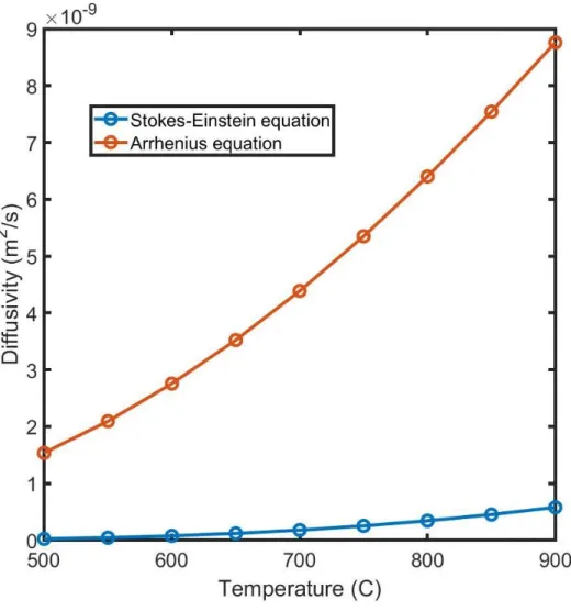
This model calculates diffusivity by coupling viscosity with activity data in melts. However, activity of chromium in aluminum melts are not available in literature. For the present study, predictions of Stokes-Einstein and Arrhenius equations are investigated to highlight the sensitivity of diffusivity on incubation times,

35

Figure 2.5: Diffusivities estimated from activity of 0.2 wt% Cr measured using Stoke-Einstein

and Arrhenius models.

There is considerable variation in the diffusivities predicted by the Stoke-Einstein and the Arrhenius models. Their variation with temperature is also significantly different, with a higher divergence seen as temperature increases. Figure 2.6 shows how these models affect the incubation time.

36

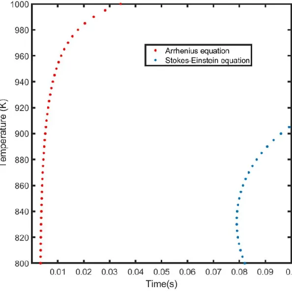
Figure 2.6: Incubation time vs temperature diagram of the nucleation times of Al13Cr2 phase

for 0.2 at % Cr. Two different diffusivity models: Arrhenius; Stokes-Einstein are compared. At 900K, the incubation times predicted by the Arrhenius and the Stokes-Einstein model are 0.0051s and 0.0992s respectively. As temperature increases, a larger divergence in the incubation times are seen. This is expected as the two models treat the liquid phase very differently. For example, The Stokes-Einstein model implicitly assumes ideal mixing in the liquid state. In the Arrhenius model, diffusion is treated as a reaction where the atom needs

37

to overcome an energy barrier to move from one point to another. Details in estimating the energy barrier are not divulged in Du et al[17].

The prediction of incubation times is heavily reliant upon the inputs provided. Diffusivity, as illustrated in Figure 2.4, is very important in prediction of incubation time. Severe lack of experimental thermodynamic data limits our understanding of the Al-Cr system. To this end, we pursued to measure activities of chromium in dilute aluminum melts using electromotive force technique. Such data can give us a better understanding of the interactions in the liquid phase of the Al-Cr system. Also, a comparative study of the predictions made with and without experimental data is presented in Chapter 5.

38

References

1. Kurz. W., Fischer. D.J. (1992). Fundamentals of Solidification. Trans Tech Publications.

2. Stefanscu.D. (2008). Science and Engineering of Casting Solidification, Springer Science.

3. Smith, P. M., Reitano, R., Aziz, M. J. (2003). Solute Trapping in metals. Retrieved from

http://www.seas.harvard.edu/matsci/people/aziz/publications/mja061.pdf%5Cnpapers2://publicati on/uuid/BAF2E23C-455C-4AE2-941F-569322FC9F43

4. Aziz, M. J. (1988). Non-equilibrium Interface Kinetics During Rapid Solidification.

5. Hoglund, D. E., & Aziz, M. J. (1992). Interface Stability during Rapid Solidification.

6. Aziz, M. J., & Kaplan. (1988). Continuous Growth Model for Interface. Materials Science and

Technology, 28(9). https://doi.org/10.1179/1743284711Y.0000000097

7. Aziz, M. J. (1994). Rapid Solidification: Growth Kinetics. The Encyclopedia of Advanced

Materials, Ed. David. Retrieved from http://dash.harvard.edu/handle/1/2961236

8. Aziz, M. J. (1996). Interface attachment kinetics in alloy solidification. Metallurgical and Materials

Transactions A: Physical Metallurgy and Materials Science, 27(3), 671–686.

https://doi.org/10.1007/BF02648954

9. Bryantsev PY, Zolotorevskiy VS, Portnoy VK (2006) The Effect of Heat Treatment and Mn, Cu

and Cr Additions on the Structure of Ingots of Al-Mg-Si-Fe Alloys. Mat. Sci. Forum. 519-521(1)

401-406.

10. Staley JT (1987) Quench factor analysis of aluminium alloys. Mat. Sci. Tech. 3(11) 923-935

11. Chinella JF, Guo Z (2011) Computational Thermodynamics Characterization of 7075, 7039, and

39

12. Li, M., Ozawa, S., & Kuribayashi, K. (2004). On determining the phase-selection principle in

solidification from undercooled melts - Competitive nucleation or competitive growth?

Philosophical Magazine Letters, 84(8), 483–493. https://doi.org/10.1080/0950083042000271090

13. Feder, J., Russell, K. C., Lothe, J., & Pound, G. M. (1966). Homogeneous nucleation and growth

of droplets in vapours. Advances in Physics (Vol. 15).

https://doi.org/10.1080/00018736600101264

14. Kashchiev D (1968) Solution of the non-steady state problem in nucleation kinetics. Surf. Sci. 14(1)

209-220

15. Porter DA, Easterling KE (1992) Phase Transformations in Metals and Alloys. Chapman & Hall

16. Shao, G., Tsakiropoulos, P., & Miodownik, A. P. (1997). Role of nucleation in phase competition in

binary Ti-Al alloys. Materials Science and Technology, 13(10), 797–805. https://doi.org/10.1179/mst.1997.13.10.797

17. Du, Y., Chang, Y. A., Huang, B., Gong, W., Jin, Z., Xu, H. (2003). Diffusion coefficients of some

solutes in fcc and liquid Al: Critical evaluation and correlation. Materials Science and Engineering

A, 363(1–2), 140–151. https://doi.org/10.1016/S0921-5093(03)00624-5

18. Thompson, C. V., & Spaepen, F. (1983). Homogeneous binary metallic melts in binary metallic melts. Acta Metall, 31(12), 2021–2027.

19. R.N. Singh and F. Sommer: Phys. Chem. Liq., 1998, vol. 36, pp. 17–28

20. Lee, S.-Y., & Iijima, Y. (1991). Diffusion of Chromium and Palladium in β-Titanium. Materials Transactions, JIM, 32(5), 451-456.

41

Chapter 3

Experimental Methods

Theory has been presented which links several thermodynamic and physical properties to incubation time, as illustrated in Equation 2.13. Unfortunately, liquid phase phenomena and transport properties of the liquid Al-Cr system have received very little experimental attention. This section explores an electrochemical method to inform high temperature thermodynamics of the Al–Cr system, by using the electrochemical potential difference (EMF) method. The The cell potential difference (E) obtained can be related to the mixing properties by using the Nernst equation.

∆𝐺

_𝐶𝑟

= −𝑧𝐹𝐸 (3.1)

where ∆𝐺_𝐶𝑟 is the chemical potential of chromium in the Al-Cr alloy with the thermodynamic reference state (pure solid chromium), z is the number of electrons per ion that travels across the cell (z=3 for Chromium (III) ion), F is Faraday’s constant.

For constructing an electrochemical cell, selection of the electrolyte is critical. An electrolyte must be ionically conductive (i.e. allow ions to dissolve and diffuse) but electronically insulating (i.e. does not allow electrons to move freely). Unfortunately, relatively few materials support the rapid ionic diffusion of cations while being electronically insulating at high temperatures in solid state. Beta(β) and beta’’(β’’) alumina solid electrolytes (BASE) presents

42

a promising class of materials for measuring thermodynamics of mixing for the Al-Cr system [2-6]. Therefore, chromium selective, alumina based electrolyte (Crβ”-Al2O3) has been

proposed as a candidate for the thermodynamic study of Al-Cr system.

3.1 Electrolyte

Several methods have been established for synthesis of BASE, ranging from powder sintering to ion exchange process. Sattar[7] proposed production of Crβ”-Al2O3 using an ion exchange

route in anhydrous CrCl under a chlorine atmosphere. This has been noted as a very slow process and it takes around 14 days for producing one batch of Crβ”-Al2O3 pellets. The

resultant pellet was physically unstable, with a lot of visible cracks. Hence, a different plan of action for synthesis of Crβ”-Al2O3 has been proposed in this study.

An alternate route for synthesizing Crβ”-Al2O3 was explored by sintering base oxides.

Reagent-grade chromium(III) oxide (Cr2O3, 99 pct pure, Sigma-Aldrich), magnesium(II) oxide

(MgO, 99.95 pct pure, Alfa Aesar), and aluminum(III) oxide (Al2O3, 99.95 pct pure, Alfa Aesar)

used in the synthesis of the solid electrolyte. A process map to prepare the solid electrolyte, illustrated in Figure 3.1.

43

Figure 3.1: Process route to solid electrolyte formation.

As evident from Figure 3.1, multiple process variables such as milling time, head pressure, sintering temperature and time need to be optimized during production of the solid electrolyte. One of the biggest difficulties of developing this process map was optimization of process variables in order to minimize cracks of the pellet.

Oxides of aluminum, chromium and magnesium were dried under vacuum for 48 hrs at 200°C. They were mixed in 31:6:4 formula unit ratio in a crucible. The powders were transferred to a micronizing mill and thoroughly mixed for 3 hours. This resultant mixture was pressed to a pressure of 110MPa. The green was sintered in a box furnace under air for ten hours, with heating and cooling rates of 3 K/min.

44

Before proceeding to cell design and electrode selection, it is important to test some functional aspects of the electrolyte at typical melt temperatures (600°C-1100°C). One important attribute for electrolyte is to be inert at high temperatures with materials of investigation. A simple compatibility test was performed with Crβ”-Al2O3 contact with pure aluminum at a

1000°C for 12 hours. The setup is cooled back to room temperature at a rate of 2C/min. The results of the compatibility tests are detailed in Section 4.1.

3.2 Cell Assembly and Procedures

For electrochemical studies to be carried out, a high temperature cell assembly has to be designed to make a electromotive force measurement. The following isothermal electrochemical cell was constructed illustrated in Figure 3.4:

Cr-Al||Crβ” Al

2

O

3

|| Ref

Where Ref (short for reference electrode) indicates two candidate compositions that were used in this study: Al-15 wt% Cr and chromium powder (99.8 pct pure, Alfa Aesar).

45

Figure 3.2: Schematic diagram of the cell for EMF measurements including cross section of

chamber containing EMF cell.

As shown by Figure 3.2, alumina tube was used as an insulating sheath. The whole set up was placed in a tube furnace made of refractory insulation equipped with vacuum feed-through fittings for movement and insertion of electrical leads. Molybdenum wires were used as current collectors to the graphite. Epoxy served as seals at the top and bottom of the alumina rods for maintaining argon atmospheres during experiment times. Alumina tubes were joined to electrolyte with the help of alumina paste. An exploded view of the reference cell is shown in Figure 3.3.

46

Figure 3.3: a) Cross section and b) Top view of EMF cell comprised of reference metal

(Chromium alloy) in the Crβ” Alumina solid electrolyte to be immersed in liquid Al-Cr.

The alumina tube (ID 6.5 cm) containing the solid chromium (RE) was joined to the Crβ” Al2O3

solid electrolyte (11mm, thickness 3.2mm) with alumina paste. This vessel was submerged in an aluminum-chromium sample of known composition to complete the cell assembly. The working electrode melt compositions studies are as follows:

Composition ID 1 2 3 4 5

Melt Composition (wt. % Cr) 0.1 0.2 0.4 0.6 0.75

47

3.2.1 Procedure for EMF Measurements:

For each EMF measurement, the following procedure was followed:

1) Chromium-aluminum alloy samples listed in Table 3.2 were prepared from chromium powder (99.8 pct pure, Alfa Aesar) and aluminum (99.99 pct pure, Alfa Aesar). Chromium powder was placed in the reference electrode vessel and the setup is assembled inside the tube furnace.

2) Before EMF measurements, the furnace temperature controller was calibrated during the compatibility testing with a R-type thermocouple to ensure temperature accuracy. The controller was set at a temperature of 1100°C, with a ramp rate of 2K/min. 3) After holding the sample at the target temperature, the reference electrode vessel

(Figure 3.3) was lowered between 2mm-3mm into the melt to complete the cell assembly.

4) The raw EMF data was acquired at a frequency of 10 Hz using a potentiostat (Gamry Instruments). A holding time at the target temperature of 1800-2400 seconds was allowed, to ensure a steady EMF reading.

5) After acquiring raw EMF reading at the target temperature, the electrode vessel was removed from the melt. After this, the temperature was ramped down at a rate of 2 K/min. Steps 3-5 are repeated at every 50K temperature interval, as the melt is cooled down.

The above procedure was followed for all working electrode compositions. The acquired raw EMF data were fitted linearly in this temperature range, as detailed in Section 4.2.

48

3.2.2 Metallographic Techniques for EMF materials:

Electrolyte:

Crβ” Alumina was machined to an outer diameter of 10mm using a Dremel rotary kit. The sample was cold mounted with an epoxy resin and cured for 24 hours. After curing, the sample was grinded with sand paper. To verify the electrolyte composition, a scanning electron microscope (SEM, JEOL JSM-6610LV, JEOL Ltd.) with an energy dispersion spectroscopy analyzer (Sirius SD detector) was used (refer Table 4.1).

Compatibility test:

The cross section of the solidified sample compatibility test was cold mounted using an epoxy resin and cured for 24 hours. After grinding the sample with sand paper, a composition study was performed using scanning electron microscope (SEM, JEOL JSM-6610LV). Spot composition was acquired at every 5 micron intervals along the length of the metal-electrolyte interface. The results are presented in Section 4.1.

49

3.3 V-shaped mold cast

An Al-0.5 wt% Cr alloy is solidified with a proprietary copper mold at Solatens Technology Center (Spokane, WA, USA). The copper mold is V-shaped, thereby achieving cooling rates that are different along the depth of the mold (Schematic shown in Figure 3.6).

Figure 3.4: Cross section of a V-shaped mold and corresponding cooling rates are mapped

here. 1 10 100 1000 10000 100000 0 0.2 0.4 0.6 0.8 1 1.2 Solid if icatio n Rat e (C/s )

50

3.3.1

Metallographic techniques:

Sample Preparation:

Thin slices were cut from the as-cast ingot at two cooling rates: 30K/s and 4600K/s. The samples were shipped to Massachusetts Institute of Technology for metallographic analysis. Samples cast from V mold were obtained from Solatens technology center. cut using a band saw and mounted in KonductoMet phenolic compound. The mount was polished to a mirror finish with 0.05 micron colloidal silica. The samples were etched with Weck’s reagent (4g of KMnO4, 1 g of NaOH and 100mL of distilled water).

Optical Microscopy:

Olympus gx51 optical microscope was used for imaging etched samples with a 10x-500x objective lenses. The etchant was capable of highlighting variations in compositions across the microstructure. Both polarized and normal light settings were used in analyzing the microstructure of the sample. The chromium rich regions were etched and grain boundaries were brighter than the matrix when viewed under polarized light. A Olympus camera and Streams essentials software was used for image acquisition.

SEM:

For composition studies, a JEOL JXA-8200 Superprobe scanning electron microscopy equipped with a wavelength dispersive spectrometer was used. A 15kV accelerating voltage was used for analyzing the samples. WDS studies confirmed the presence of hexagonal shaped Al13Cr2 precipitates in slowly solidified (30K/s) cast sample (refer Figure 7.1 in

52

References

1. Fries, S., & Lukas, H. L. (1998). COST 507 Definition of thermochemical and Thermochemical

database for light metal alloys. (Vol. 2).

2. Little, J. A., & Fray, D. J. (1980). The Preparation and Properties of Copper Beta Alumina.

Electrochimia Acta, 25, 957–964.

3. Chowdhury, M. T., Takekawa, R., Iwai, Y., Kuwata, N., & Kawamura, J. (2014). Lithium ion diffusion

in Li β-alumina single crystals measured by pulsed field gradient NMR spectroscopy. Journal of

Chemical Physics, 140(12). https://doi.org/10.1063/1.4869347

4. Fray, D. J. (1977). Determination of sodium in molten aluminum and aluminum alloys using a beta

alumina probe. Metallurgical Transactions B, 8(1), 153–156. https://doi.org/10.1007/BF02656364 5. Cleaver, B., & Davies, A. J. (1973). PROPERTIES OF FUSED POLYSULPHIDES-III. EA4F

MEASUREMENTS ON THE SODIUM-SULPHUR CELL, AND SULPHUR ACTIVITIES AND

CONSTITUTION IN FUSED SODIUM POLYSULPHIDES. Electrochemica Acta, 18(I), 733–739. 6. Oishi, T., Tagawa, S., & Tanegashima, S. (2005). Thermodynamic study of solid copper-nickel

alloys by use of copper-beta-alumina. Journal of Physics and Chemistry of Solids, 66(2–4), 251– 255. https://doi.org/10.1016/j.jpcs.2004.08.038

7. Sattar, S., Ghosal, B., Underwood, M. L., Mertwoy, H., Saltzberg, M. A., Frydrych, W. S., Farrington,

G. C. (1986). Synthesis of di- and trivalent β″-aluminas by ion exchange. Journal of Solid State

54

Chapter 4

Experimental Results

Crβ” alumina was synthesized using sintering of oxide components. The diameter of the resultant pellet was 32 mm, with a thickness of 3.1mm. The image of the final product is shown in Figure 4.1.

Figure 4.1: Crβ” Alumina solid electrolyte synthesized directly from Cr2O3, MgO and Al2O3

55

The pellet has changed color to pinkish brown color after sintering. There was no cracking of pellet post sintering. Machining of sintered product was similar to alumina, indicating good structural stability in air.

Before conducting measurements, compatibility testing (indicated in Section 3.1) was performed. The cross section of the solidified sample compatibility test is shown in Figure 4.2.

Figure 4.2: Cross section of graphite containing Crβ”-Al2O3 and aluminum after compatibility

test.

As indicated in Figure 4.2, a cursory eye test indicates that aluminum wets the electrolyte better than graphite crucible. There is no change in color or visible penetration of aluminum into the electrolyte. In general, what we can see is that there is good adhesion between the electrolyte and solidified aluminum. Bulk composition analysis of the electrolyte was obtained

56

and the results are summarized in Table 4.1. SEM-EDS composition measurement of the metals (Al, Cr, Mg) were obtained and their corresponding oxide weights are reported in Table 4.1.

Powder Composition before test (wt%) Composition after test (wt%)

Al2O3 87.2 87.4

Cr2O3 8.4 8.3

MgO 4.4 4.3

Table 4.1: Composition of oxides that are sintered to form Crβ” Alumina solid electrolyte.

There is very good composition integrity that is observed pre and post compatibility test. Also, no macro cracks were observed in the membrane, indicating sound structural stability under challenging thermal conditions. The next analysis that was performed was a spot composition at every 5 micron intervals along the length of the metal-electrolyte interface. For perspective, Figure 4.3 provides the visual representation of the interface and composition map of this region.

57

(a)

(b)

Figure 4.3: (a) Schematic of metal-electrolyte interface. (b) Composition of chromium oxide

58

From Figure 4.3 (b), no contamination of chromium in the aluminum side of the interface is found. Also, the chromium content of the electrolyte is preserved. Therefore, compatibility test proves that membrane can withstand high temperatures without decomposing or losing structural stability. The results of the compatibility test can be summarized as:

(i) The electrolyte can withstand high temperatures without decomposing or losing structural stability.

(ii) Insignificant amount of Cr contamination in pure aluminum confirms compositional integrity of the electrolyte.

59

4.1 EMF measurements:

Section 3.2.1 detailed the procedure used for acquiring raw EMF data from the Al-Cr alloy vs Cr cell with Crβ”-Al2O3 used as the solid electrolyte. Before analyzing cell assembly and EMF

measurements, a representative raw EMF vs time data collected for Al-0.75 wt% Cr vs Cr using Crβ”-Al2O3 solid electrolyte is shown in Figure 4.4.

Figure 4.4: Sample of raw EMF data for 0.75 wt % Cr vs Cr using Crβ”-Al2O3 solid electrolyte

at 1323K.

At a given temperature, steady state in EMF readings were typically reached within 2400 seconds. After stabilization, EMF readings for a time period of 120 seconds were acquired. The average of this data set is reported as the EMF measurement for the given temperature. Standard deviations in EMF measurements generally ranged from 0.05 to 0.3 mV. A longer

60

hold time (~3600 seconds) were required for stabilization. After data acquisition, the temperature is cooled down at a rate of 2K/min until the new target temperature is reached. After repeating this procedure for five compositions, variation of electrochemical potential with temperature and their liquidus temperatures are reported in Tables 4.2 and 4.3 respectively. The reported values of EMF have a standard deviation of less than 0.5mV, unless explicitly mentioned.

Wt %

Cr

EMF (mV)

750°C 800°C 850°C 900°C

950°C 1000°C 1050°C 1100°C

0.1

427.1*

-

460.9

-

500.6* 505.2

540.4

-

0.2

-

-

397.5 410.1* 425.7

440.8

444.9

-

0.4

345.2 352.1* 362.1

-

385.5

-

405.4

-

0.6

310.4* 325.6

332.3 335.3* 340.5

351.1

364.6

370.6

0.75

-

-

-

-

319.2

320.8

330.1

336.8

Table 4.2: Measured EMF values for five compositions of interest. (Star marks next to EMF

values indicates that standard deviation of reported values are less than 1mV).

Wt % Cr Measured liquidus (°C ) EMF (mV) 0.1 665 401.2* 0.2 686 358.4* 0.4 696 332.1* 0.6 706 305.6* 0.75 720 289*

Table 4.3: Measured liquidus values for five compositions of interest. (Star marks next to

61

The EMF readings for each compositions are fit according to the following expression (Table 4.4).

𝐸 = 𝐴𝑇 + 𝐵

(4.1)

𝐴 =

𝜕𝐸 𝜕𝑇

(4.2)

Wt % Cr

A (× 10

-3

_{V K}

-1

_{) B (× 10}

-3

_V)

0.10

0.3215

187.4

0.20

0.246

189.6

0.40

0.2056

188.9

0.60

0.1612

191.8

0.75

0.122

201.2

Table 4.4: Parameters calculated from a linear interpolation of measured EMF data with

temperature.

A graphical representation of the tabulated data is shown in Figure 4.5. For 0.75 wt% Cr, potentials failed to stabilize below the cut off limit around 900C as depicted in Figure 4.5.

62

Figure 4.5: Variation of the electrochemical potential with temperature for five compositions.

Triangular data points represent measured liquidus at each composition. EMF values without star marks indicates that standard deviation of reported values are less than 0.5mV. Star marks next to EMF values indicates that standard deviation of reported values are less than 1mV.

EMF measurements can be converted to corresponding activities of Cr by Equation 4.3.

𝑎

_{𝐶𝑟 (𝑖𝑛 𝐴𝑙)}

= 𝑒

−3𝐹𝐸/𝑅𝑇

(4.3)

63

Figure 4.6: Activity coefficients of Cr for five compositions calculated from electrochemical

potential data. . EMF values without star marks indicates that standard deviation of reported values are less than 0.5mV. Star marks next to EMF values indicates that standard deviation of reported values are less than 1mV.

Activity coefficients at the dilute regime can be estimated from the following equation. The values of parameters are listed in Table 4.5.

ln 𝛾

𝐶𝑟

= 𝐶 + 𝐷𝑥

𝐶𝑟

(4.5)

𝐷 = [

𝜕 𝑙𝑛 𝛾𝐶𝑟

𝜕𝑥_𝐶𝑟

]

_𝑥

𝐶𝑟→0

64

T(C)

C

D

750

-7.337

826.9

850

-6.601

707.6

950

-6.508

789.3

1050

-5.408

533.4

Table 4.5: Parameters calculated from a linear interpolation of activity coefficients with

composition.

From Figure 4.6, the value of activity coefficient of Al-0.1wt% Cr at 950°C can be determined to be 0.0014. Remarkably, the aluminum-thorium(Al-Th) system[1] also shows similarly low activity coefficients of thorium (4.5 × 10-5 _{at 1050°C)[2] in the dilute limits. However, minimal}

experimental efforts have been directed for comparison of activity coefficients for other dilute liquid aluminum alloy melts. Nevertheless, such low values of activity coefficients are not entirely surprising, considering the tendency of chromium to form intermetallic compounds with aluminum. Also, the temperature range of interest for this study here lies significantly below the melting point of chromium, thereby increasing the tendency of chromium to exist in the solid state. Ultimately, the lower values of activity coefficients of chromium indicate a pronounced deviation from Raoultian ideality.

66

References

1. Kassner, M. E., & Peterson, D. E. (1989). The Al-Th (Aluminum-Thorium) system. Bulletin of Alloy

Phase Diagrams, 10(4), 466–470. https://doi.org/10.1007/BF02882381

2. Hultgren, R., & Desai, P. D. (1973). Selected Values of the Thermodynamic Properties of Binary

68

Chapter 5

Predictions of impact of cooling rates on

solidification

Recalling the analysis on diffusivity models, incubation times are evaluated with the new activity data (Figure 5.1). Case 1 was based on Arrhenius (Equation 2.17) model of diffusivity.

Figure 5.1: Incubation time vs temperature diagram of the nucleation times of Al13Cr2 phase

69

Case 2 assumed that Stokes-Einstein model can be used to model diffusivity to be (Eq 2.18). Case 3 was computed with activity data obtained from this study, diffusion coefficients can now be obtained using the experimental Singh-Sommer relation (Equation 2.20).

As shown in Figure 5.1, the Stokes-Einstein model predicts higher incubation times, than the other two models throughout the temperature range. This may be stemming from the implicit assumption that Gibbs energies of mixing is ideal. Arrhenius model predicts much lower incubation times, however, no details are divulged in Hu et al[2] on the estimation of activation energy of chromium in liquid aluminum. Neither model accounts for strong negative deviations from ideality of the aluminum-chromium system, as evident from the activity data. For the prediction of diffusivities using the Singh-Sommer relation, linear interpolations of measured activity with temperature were utilized. Incubation times predicted by the Singh-Sommer model lie in between the predictions of the former model. While experimental diffusivity values are unavailable in literature, incorporating measured activities in the Singh-Sommer relation provide better estimates of diffusivity of chromium diffusion in liquid aluminum-chromium melts.

5.1 Features of

∆t vs T diagram:

The natural continuation of the discussion explores of a ∆t vs T diagram. By using this tool, incubation times of multiple competing phases can be mapped onto a single plot, as shown in Figure 5.2 comparing Al13Cr2 and α-Al phase (α).

70

Figure 5.2: Incubation time vs temperature diagram of the nucleation times of the two phases

for 0.5 wt % Cr. The blue points corresponds to Al13Cr2 (γ) while the orange points to α-Al

phase (α).

Incubation times at high temperatures tend to be very large. This is expected as the driving force for nucleation is low. As the temperature decreases, the time required for nucleation decreases until a minimum is reached. Further decrease in temperature results in increase of incubation time (below 600°C), as kinetics becomes sluggish due to suppression of mobility.

Cooling rates (ε) can be directly mapped on a ∆t vs T diagram. It is expressed as an absolute value of the ratio of undercooling (∆𝑇) and incubation time (∆𝑡)

𝜀 = |

∆𝑇

71

Figure 5.3: Incubation time vs temperature diagram of the Al13Cr2 phase 0.5 wt % Cr. Alloy

is initially superheated to a temperature (TS) around 50K above their liquidus (TL) and cooled

down.

A point of consideration is specification of the superheat temperatures. In order to simulate real casting conditions, alloys are commonly superheated to 50K higher temperature than their liquidus temperatures. While this is a good approximation for the subject of this investigation, this temperature can vary based on casting practices and available cooling technologies. Three different cooling rates are imposed in Figure 5.4, to show that cooling rates indeed primary phase selection during solidification.

72

Figure 5.4: Incubation time vs temperature diagram of the nucleation times of the two phases

for 0.5 wt % Cr. The blue points corresponds to Al13Cr2 (γ) while the orange points to α-Al

phase (α). This alloy is subject to three different cooling rates: ε1 < εc < ε2.

At cooling rate of ε1, it is seen that the incubation time for Al13Cr2 is lower than the α-Al. This

prediction is in tune with the fact that low cooling rates lead to formation of intermetallic phase, as indicated by the equilibrium phase diagram. At sufficiently high cooling rate ε2, there exists

a possibility of nucleating α-Al preferentially over Al13Cr2. As discussed previously in Chapter

1, non-equilibrium solidification conditions may lead to suppression of intermetallic phase. Another point to note is that there exists a critical cooling rate beyond which kinetics hinders

73

formation of the thermodynamically favored phase. Mathematically, εc is the cooling rate at

which the ∆t(α-Al) = ∆t(Al13Cr2). This presents the two following scenarios:

𝜀 < 𝜀_𝑐  Al13Cr2 forms preferentially

𝜀 > 𝜀𝑐  α-Al forms preferentially

Therefore, cooling rates can be used to suppress phase formation that is typical of equilibrium conditions, thereby enabling a higher degree of supersaturation. Incubation time vs temperature diagrams are very useful in understanding solidification path taken for different cooling rates. This allows us to determine critical cooling rates for suppressing the nucleation of the intermetallic phase.

For establishing standards for comparing capabilities of casting technologies, characteristic cooling rates have been used in this study. Therefore, one may provide detailed input parameters to emulate a more realistic picture of a specific casting technology. Let

ε

_𝑝 represent the characteristic cooling rate of a casting process. If

𝜀

_𝑝

> ε

_𝑐 , α-Al is selected as the primary phase. Figure 5.1 shows that DC casting of 0.1 wt% Cr alloy results in intermetallic formation (𝜀𝐷𝐶 =10K/s) owing to lower cooling rates. Cooling rate for twin roll

casting (𝜀_𝑇𝑅 =1000K/s) is greater than the critical value for this composition, suggesting α-Al nucleation as the primary phase.