Any correspondence concerning this service should be sent to the repository administrator:
[email protected]
O
pen
A
rchive
T
oulouse
A
rchive
O
uverte (
OATAO
)
OATAO is an open access repository that collects the work of Toulouse researchers and
makes it freely available over the web where possible.
This is an author-deposited version published in:
http://oatao.univ-toulouse.fr/
Eprints ID: 8942
To link to this article
DOI:10.1109/TSP.2013.2245127
http://dx.doi.org/10.1109/TSP.2013.2245127
To cite this version:
Altmann, Yoan and Dobigeon, Nicolas and McLaughlin, Steve and Tourneret,
Jean-Yves Nonlinear spectral unmixing of hyperspectral images using Gaussian
processes. (2013) IEEE Trans. Signal Processing, vol. 61 (n° 10). pp.
Nonlinear Spectral Unmixing of Hyperspectral
Images Using Gaussian Processes
Yoann Altmann, Student Member, IEEE, Nicolas Dobigeon, Member, IEEE, Steve McLaughlin, Fellow, IEEE, and
Jean-Yves Tourneret, Senior Member, IEEE
Abstract—This paper presents an unsupervised algorithm for
nonlinear unmixing of hyperspectral images. The proposed model assumes that the pixel reßectances result from a nonlinear function of the abundance vectors associated with the pure spectral nents. We assume that the spectral signatures of the pure compo-nents and the nonlinear function are unknown. The Þrst step of the proposed method estimates the abundance vectors for all the image pixels using a Bayesian approach an a Gaussian process latent vari-able model for the nonlinear function (relating the abundance vec-tors to the observations). The endmembers are subsequently esti-mated using Gaussian process regression. The performance of the unmixing strategy is Þrst evaluated on synthetic data. The pro-posed method provides accurate abundance and endmember es-timations when compared to other linear and nonlinear unmixing strategies. An interesting property is its robustness to the absence of pure pixels in the image. The analysis of a real hyperspectral image shows results that are in good agreement with state of the art unmixing strategies and with a recent classiÞcation method.
Index Terms—Gaussian processes, hyperspectral imaging,
spec-tral unmixing.
I. INTRODUCTION
S
PECTRAL UNMIXING (SU) is a major issue whenanalyzing hyperspectral images. It consists of identifying the macroscopic materials present in an hyperspectral image and quantifying the proportions of these materials in the image pixels. Many SU strategies assume that pixel reßectances are linear combinations of pure component spectra [1]–[4]. The resulting linear mixing model (LMM) has been widely adopted in the literature and has provided some interesting results. How-ever, as discussed in [1], the LMM can be inappropriate for some hyperspectral images. Nonlinear mixing models provide an interesting alternative to overcome the inherent limitations of the LMM. For instance, the presence of relief can induce mul-tiple scattering effects between the different materials presentY. Altmann, N. Dobigeon, and J.-Y. Tourneret are with the University of Toulouse, IRIT-ENSEEIHT, Toulouse 31071, France (e-mail: [email protected]; [email protected]; [email protected]).
S. McLaughlin is with the School of Engineering and Physical Sci-ences, Heriot-Watt University, Edinburgh EH14 4AS, U.K. (e-mail: [email protected]).
Digital Object IdentiÞer 10.1109/TSP.2013.2245127
in the image. These nonlinear scattering effects typically occur in vegetation areas [5] and urban scenes [6]. A speciÞc class of nonlinear models referred to as bilinear models has been studied in [5], [7]–[9] for modeling these multiple scattering effects. Conversely, the bidirectional reßectance-based model of [10] focusses on hyperspectral images including intimate mixtures, i.e., when the pure spectral components do not sit side-by-side in the pixel and when the photons are then inter-acting with all the materials simultaneously. These intimate mixtures can occur in sand-like or mineral areas. Other more ßexible unmixing techniques have been also proposed to handle wider classes of nonlinearities, including radial basis function networks [11], [12] post-nonlinear mixing models [13] and kernel-based models [14]–[17].
Most existing unmixing strategies can be decomposed into two steps referred to as endmember extraction and abundance estimation. Endmember identiÞcation is usually achieved be-fore estimating the abundances for all the image pixels. In the last decade, many endmember extraction algorithms (EEAs) have been developed to identify the pure spectral components contained in a hyperspectral image (see [1] for a recent review of these methods). Most EEAs rely on the LMM, which, as dis-cussed, is inappropriate for the case of nonlinear mixtures of the endmembers. More recently, an EEA was proposed in [18] to extract endmembers from a set of nonlinearly mixed pixels. The nonparametric approach proposed in [18] was based on the assumption that the observed pixels lie on a manifold and that the endmembers are extreme points of this manifold. An approx-imation of the geodesic distance associated with this manifold was then used to identify the endmembers from the data. Simi-larly, our approach assumes that the data lie on a (possibly non-linear) manifold. However, this paper proposes a parametriza-tion of the manifold through the use of a kernel. The main ad-vantages of this kernel-based parametric approach are 1) a better description of the manifold when the number of image pixels is reduced, and 2) a better endmember identiÞcation when there is no pure pixel in the image. This paper proposes Þrst to es-timate the abundance vectors and to eses-timate the endmembers during a second step, using the prediction capacity of Gaussian processes (GPs). This approach breaks from the usual paradigm of spectral unmixing. More precisely, this paper considers a kernel-based approach for nonlinear SU based on a nonlinear di-mensionality reduction using a Gaussian process latent variable model (GPLVM). The main advantage of GPLVMs is their ca-pacity to accurately model many different nonlinearities. In this paper, we propose to use a particular form of kernel based on existing bilinear models, which allows the proposed unmixing strategy to be accurate when the underlying mixing model is bi-linear. Note that the LMM is a particular bilinear model. The algorithm proposed herein is “unsupervised” in the sense that
the endmembers contained in the image and the mixing model are not known. Only the number of endmembers is assumed to be known. As a consequence, the parameters to be estimated are the kernel parameters, the endmember spectra and the abun-dances for all image pixels.
The paper is organized as follows. Section II presents the non-linear mixing model considered in this paper for hyperspectral image unmixing. Section III introduces the GPLVM used for la-tent variable estimation. A constrained GPLVM for abundance estimation is detailed in Section IV. Section V studies the end-member estimation procedure using GP regression. Some sim-ulation results conducted on synthetic and real data are shown and discussed in Sections VI and VII. Finally, conclusions are drawn in Section VIII.
II. NONLINEARMIXINGMODEL
Consider a hyperspectral image of pixels, composed of endmembers and observed in spectral bands. For convenience, the data are assumed to have been previously centered, i.e., the sample mean of the original pixels has been subtracted from each observed pixel. The
-spec-trum of the th mixed pixel
is deÞned as a transformation of its
corre-sponding abundance vector as
follows
(1) where is a linear or nonlinear unknown func-tion. The noise vector is an independent, identically dis-tributed (i.i.d.) white Gaussian noise sequence with variance ,
i.e., , . Without loss
generality, the nonlinear mapping (1) from the abundance space to the observation space can be rewritten
(2) where , is an matrix and the dimension is the dimension of the subspace spanned by the transformed abundance vectors , . Of course, the per-formance of the unmixing strategy relies on the choice of the nonlinear function . In this paper, we will use the following nonlinearity
(3) with . The primary motivation for considering this particular kind of nonlinearity is the fact that the resulting mixing model is a bilinear model with respect to each abundance , . More precisely, this mixing model extends the generalized bilinear model proposed in [9] and thus the LMM. It is important to note from (2) and (3) that contains the spectra of the pure components present in the image and
interaction spectra between these components. Note also that the analysis presented in this paper could be applied to any other nonlinearity .
Due to physical constraints, the abundance vector satisÞes the following posi-tivity and sum-to-one constraints
(4) Since the nonlinearity is Þxed, the problem of unsupervised spectral unmixing is to determine the spectrum matrix
, the abundance matrix
satisfying (2) under the constraints (4) and the noise variance . Unfortunately, it can be shown that the solution of this con-strained problem is not unique. In the noise-free linear case, it is well known that the data are contained in a simplex whose ver-tices are the endmembers. When estimating the endmembers in the linear case, a simplex of minimum volume embedding the data is expected. Equivalently, the estimated abundance vectors are expected to occupy the largest volume in the simplex de-Þned by (4). In a similar fashion to the linear case, the estimated abundance matrix resulting from an unsupervised nonlinear SU strategy may not occupy the largest volume in the simplex de-Þned by (4). To tackle this problem, we Þrst propose to relax the positivity constraints for the elements of the matrix and to consider only the sum-to-one constraint. For ease of under-standing, we introduce vectors satisfying the sum-to-one constraint
(5) referred to as latent variables and denoted as
, . The positivity
con-straint will be handled subsequently by a scaling procedure discussed in Section IV. The next section presents the Bayesian model for latent variable estimation using GPLVMs.
III. BAYESIANMODEL
GPLVMs [19] are powerful tools for probabilistic nonlinear dimensionality reduction that rewrite the nonlinear model (1) as a nonlinear mapping from a latent space to the observation space as follows
(6)
where is deÞned in (3), is an
matrix with , and .
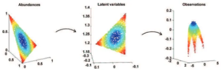
Note that from (2) and (6) the columns of span the same subspace as the columns of . Consequently, the columns of are linear combinations of the spectra of interest, i.e., the columns of . Note also that when is full rank, it can be shown that the latent variables are necessarily linear combina-tions of the abundance vectors of interest. Figs. 1 and 2 illustrate the mapping from the abundance vectors to the observations that will be used in this paper. Note that the linear mapping be-tween the abundances and the latent variables will be explained in detail in Section IV. For brevity, the vectors
will be denoted as in the sequel. Assuming independence between the observations, the statistical properties of the noise
Fig. 1. Nonlinear mapping from the abundances vectors to the observed mixed pixels.
Fig. 2. Example of mapping decomposition from the abundance vectors to the observed nonlinearly mixed pixels through the latent variables .
lead to the following likelihood of the observation matrix
(7)
where is the latent variable
matrix. Note that the likelihood can be rewritten as a product of Gaussian distributions over the spectral bands as follows
(8)
where and is
an matrix. The idea of GPLVMs is to consider as a nuisance parameter, to assign a Gaussian prior to and to marginalize the joint likelihood (7) over , i.e.,
(9) where is the prior distribution of . The estimation of and can then be achieved by maximizing (9) following the maximum likelihood estimator (MLE) principle. An alternative consists of using an appropriate prior distribution , as-suming prior independence between and , and max-imizing the joint posterior distribution
(10) with respect to (w.r.t.) , yielding the maximum a poste-riori (MAP) estimator of . The next paragraph discusses different possibilities for marginalizing the joint likelihood (8) w.r.t. .
A. Marginalizing
It can be seen from (9) that the marginalized likelihood and thus the associated latent variables depend on the choice of the
prior . More precisely, assigning a given prior for fa-vors particular representations of the data, i.e., particular solu-tions for the latent variable matrix maximizing the posterior (10). When using GPLVMs for dimensionality reduction, a clas-sical choice [19] consists of assigning independent Gaussian priors for , leading to
(11) However, this choice can be inappropriate for SU. First, (11) can be incompatible with the admissible latent space, constrained by (5). Second, the prior (11) assumes the columns of (linear combinations of the spectra of interest) are a priori Gaussian, which is not relevant for real spectra in most applications. A more sophisticated choice consists of considering a priori corre-lation between the columns (inter-spectra correcorre-lation) and rows (inter-bands correlation) of using a structured covariance matrix to be Þxed or estimated. In particular, introducing cor-relation between close spectral bands is of particular interest in hyperspectral imagery. Structured covariance matrices have already been considered in the GP literature for vector-valued kernels [20] (see [21] for a recent review). However, computing the resulting marginalized likelihood usually requires the esti-mation of the structured covariance matrix and the inversion of an covariance matrix,1which is prohibitive for
SU of hyperspectral images since several hundreds of spectral bands are usually considered when analyzing real data. Sparse approximation techniques might be used to reduce this compu-tational complexity (see [23] for a recent review). However, to our knowledge, these techniques rely on the inversion of ma-trices bigger than matrices. The next section presents an alternative that only requires the inversion of an covari-ance matrix without any approximation.
B. Subspace IdentiÞcation
It can be seen from (6) that in the noise-free case, the data belong to a -dimensional subspace that is spanned by the columns of . To reduce the computational complexity induced by the marginalization of the matrix while con-sidering correlations between spectral bands, we propose to marginalize a basis of the subspace spanned by instead of
itself. More precisely, can be decomposed as follows (12)
where is an matrix ( is vector)
whose columns are arbitrary basis vectors of the -dimensional subspace that contains the subspace spanned by the columns of
and is a matrix that scales the
columns of . Note that the subspaces spanned by and are the same when is full rank, resulting in a full rank matrix . The joint likelihood (8) can be rewritten as
(13)
where is an matrix. The proposed subspace estimation procedure consists of assigning an appropriate prior distribution to (denoted as ) and to marginalize from the joint posterior of interest. It is easier to choose an infor-mative prior distribution that accounts for correlation be-tween spectral bands than choosing an informative since is an arbitrary basis of the subspace spanned by , which can be easily estimated (as will be shown in the next section).
C. Parameter Priors
GPLVMs construct a smooth mapping from the latent space to the observation space that preserves dissimilarities [24]. In the SU context, it means that pixels that are spectrally different have different latent variables and thus different abundance vec-tors. However, preserving local distances is also interesting: spectrally close pixels are expected to have similar abundance vectors and thus similar latent variables. Several approaches have been proposed to preserve similarities, including back-constraints [24], dynamical models [25] and locally linear em-bedding (LLE) [26]. In this paper, we use LLE to assign an ap-propriate prior to . First, the nearest neighbors
of each observation vector are computed using the Eu-clidian distance ( is the set of integers such that is a neighbor of ). The weight matrix of size providing the best reconstruction of from its neigh-bors is then estimated as
(14) Note that the solution of (14) is easy to obtain in closed form since the criterion to optimize is a quadratic function of . Note also that the matrix is sparse since each pixel is only described by its nearest neighbors. The locally linear patches obtained by the LLE can then be used to set the following prior for the latent variable matrix
(15) where is a hyperparameter to be adjusted and is the indicator function over the set deÞned by the constraints (5). In this paper, we propose to assign a prior to using the standard principal component analysis (PCA) (note again that the data have been centered). Assuming prior independence be-tween , the following prior is considered for
(16)
where is an projection matrix
con-taining the Þrst eigenvectors of the sample covariance matrix of the observations (provided by PCA) and is a dispersion parameter that controls the dispersion of the prior. Note that the correlation between spectral bands is implicitly introduced through .
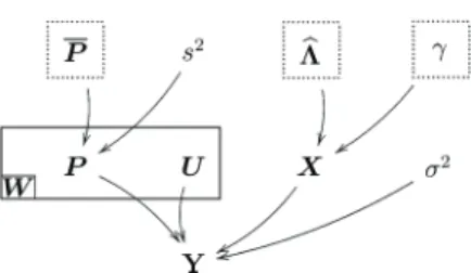
Fig. 3. DAG for the parameter priors and hyperpriors (the Þxed parameters appear in dashed boxes).
Non-informative priors are assigned to the noise variance and the matrix , i.e,
(17) where the intervals and cover the possible values of the parameters and . Similarly, the following non-informative prior is assigned to the hyperparameter
(18) where the interval covers the possible values of the hy-perparameter . The resulting directed acyclic graph (DAG) is depicted in Fig. 3.
D. Marginalized Posterior Distribution
Assuming prior independence between , , , and , the marginalized posterior distribution of
can be expressed as
(19)
where .
Straightforward computations leads to
(20)
where , is an vector,
is an matrix and denotes the matrix trace.
Mainly due to the nonlinearity introduced through the non-linear mapping, a closed form expression for the parameters maximizing the joint posterior distribution (19) is impossible to obtain. We propose to use a scaled conjugate gradient (SCG) method to maximize the marginalized log-posterior. To en-sure the sum-to-one constraint for , the following arbitrary reparametrization
is used and the marginalized posterior distribution is optimized w.r.t. the Þrst columns of denoted . The par-tial derivatives of the log-posterior w.r.t. and are obtained using partial derivatives w.r.t. and and the clas-sical chain rules (see technical report [22] for further details). The resulting latent variable estimation procedure is referred to as locally linear GPLVM (LL-GPLVM).
Note that the marginalized likelihood reduces to the product of independent Gaussian probability density functions since
(21) and . Note also that the covariance matrix
is related to the covariance matrix of the 2nd order polynomial kernel [27, p. 89]. More precisely, the proposed non-linear mapping corresponds to a particular polynomial kernel whose metric is induced by the matrix . Finally, note that the evaluation of the marginalized likelihood (20) only requires the inversion of the covariance matrix . It can been seen from the following Woodbury matrix identity [28]
(22) that the computation of mainly relies on the inversion of a matrix. Similarly, the computation of
mainly consists of computing the determinant of a ma-trix, which reduces the computational cost when compared to the structured covariance matrix based approach presented in Section III-A.
E. Estimation of
Let us denote as the maximum a poste-riori (MAP) estimator of obtained by max-imizing (19). Using the likelihood (13), the prior distribution (16) and Bayes’ rule, we obtain the posterior distribution of conditioned upon , i.e.,
(23)
where and .
Since the conditional posterior distribution of is the product of independent Gaussian distributions, the MAP estimator of
conditioned upon is given by
(24)
where , ,
and . The next
section studies a scaling procedure that estimates the abundance matrix using the estimated latent variables resulting from the maximization of (19).
IV. SCALINGPROCEDURE
The optimization procedure presented in Section III-D pro-vides a set of latent variables that represent the data but can differ from the abundance vectors of interest. Consider
obtained after maximization of the pos-terior (19). The purpose of this section is to estimate an
abundance matrix such that
(25)
where occupy the maximal volume in the
sim-plex deÞned by (4), is an
matrix and is an standard i.i.d Gaussian noise matrix which models the scaling errors. Since the rows of satisfy the sum-to-one constraint (5), estimating the relation be-tween and is equivalent to estimate the relation between
and . However, when considering the mapping between and , non-isotropic noise has to be considered since the rows of and satisfy the sum-to-one constraint, i.e., they belong to the same -dimensional subspace.
Eq. (25) corresponds to an LMM whose noisy observations are the rows of . Since is assumed to occupy the largest volume in the simplex deÞned by (4), the columns of are the vertices of the simplex of minimum volume that contains . As a consequence, it seems reasonable to use a linear un-mixing strategy for the set of vectors to es-timate and . In this paper, we propose to estimate jointly and using the Bayesian algorithm presented in [29] for unsupervised SU assuming the LMM. Note that the algorithm in [29] assumed positivity constraints for the estimated endmem-bers. Since these constraints for are unjustiÞed, the orig-inal algorithm has slightly been modiÞed by removing the trun-cations in the projected endmember priors (see [29] for details). Once the estimator of has been obtained by the proposed scaling procedure, the resulting constrained
la-tent variables denoted as are
deÞned as follows
(26) with . Using the sum-to-one constraint
, we obtain
(27)
where is an
ma-trix. The Þnal abundance estimation procedure, including the LL-GPLVM presented in Section III and the scaling procedure investigated in this section is referred to as fully constrained LL-GPVLM (FCLL-GPLVM) (a detailed algorithm is available in [22]). Once the Þnal abundance matrix and the matrix have been estimated, we propose an endmember extraction pro-cedure based on GP regression. This method is discussed in the next section.
V. GAUSSIANPROCESSREGRESSION
Endmember estimation is one of the main issues in SU. Most of the existing EEAs intend to estimate the endmembers from the data, i.e., selecting the most pure pixels in the observed image [30]–[32]. However, these approaches can be inefÞcient when the image does not contain enough pure pixels. Some other EEAs based on the minimization of the volume con-taining the data (such as the minimum volume simplex analysis [33]) can mitigate the absence of pure pixels in the image. This section studies a new endmember estimation strategy based
on GP regression for nonlinear mixtures. This strategy can be used even when the scene does not contain pure pixels. It assumes that all the image abundances have been estimated using the algorithm described in Section IV. Consider the set of pixels and the corresponding estimated abundance vectors . GP regression Þrst allows the nonlinear mapping in (1) (from the abundance space to the observation space) to be estimated. The estimated mapping is denoted as . Then, it is possible to use the prediction capacity of GPs to predict the spectrum corresponding to any new abundance vector . In particular, the predicted spectra associated with pure pixels, i.e., the endmembers, correspond to abundance vectors that are the vertices of the simplex deÞned by (4). This section provides more details about GP prediction for endmember estimation. It can be seen from the marginalized likelihood (20) that is the product of independent GPs associated with each spectral band of the data space (21). Looking carefully at the covariance matrix of
(i.e., to ), we can write
(28) where is the white Gaussian noise vector associated with the th spectral band (having covariance matrix ) and2
(29)
with the covariance matrix of
. The vector is referred to as hidden vector as-sociated with the observation . Consider now an test data with hidden vector , abundance vector
and . We assume that the
test data share the same statistical properties as the training data in the sense that is a Gaussian vector such that
(30)
where is the variance of and
contains the covariances between the training inputs and the test inputs, i.e.,
(31) Straightforward computations leads to
(32) with
Since the posterior distribution (32) is Gaussian, the MAP and MMSE estimators of equal the posterior mean
.
In order to estimate the endmembers, we propose to replace the parameters , , and by their estimates , , and and to compute the estimated hidden vectors
asso-ciated with the abundance vectors for
2Note that all known conditional parameters have been omitted for brevity.
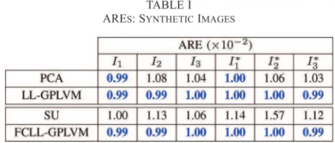
TABLE I ARES: SYNTHETICIMAGES
. For each value of , the th estimated hidden vector will be the th estimated endmember.3Indeed, for the
LMM and the bilinear models considered in this paper, the
end-members are obtained by setting in
the model (2) relating the observations to the abundances. Note that the proposed endmember estimation procedure provides the posterior distribution of each endmember via (32) which can be used to derive conÞdence intervals for the estimates. The next section presents some simulation results obtained for synthetic and real data.
VI. SIMULATIONS ONSYNTHETICDATA
A. Subspace IdentiÞcation
The performance of the proposed GPLVM for dimension-ality reduction is Þrst evaluated on three synthetic images of pixels. The endmembers contained in these images have been extracted from the spectral libraries provided with the ENVI software [34] (i.e., green grass, olive green paint and galvanized steel metal). Additional simulations conducted with different endmembers are available in [22]. The Þrst image has been generated according to the linear mixing model (LMM). The second image is distributed according to the bilinear mixing model introduced in [5], referred to as the “Fan model” (FM). The third image has been generated according to the generalized bilinear model (GBM) studied in [9] with the following nonlinearity parameters
The abundance vectors , have been randomly generated according to a uniform distribution on the admissible set deÞned by the positivity and sum-to-one constraints (4). The noise variance has been Þxed to , which corresponds to a signal-to-noise ratio which corresponds to the worst case for current spectrometers. The hyperparameter of the latent variable prior (15) has been Þxed to and the number of neighbors for the LLE is for all the results presented in this paper. The quality of dimensionality reduction of the GPLVM can be measured by the average reconstruction error (ARE) deÞned as
(33) where is the th observed pixel and its estimate. For the LL-GPLVM, the th estimated pixel is given by
where is estimated using (24). Table I compares
3Note that the estimated endmembers are centered since the data have
pre-viously been centered. The actual endmembers can be obtained by adding the empirical mean to the estimated endmembers.
Fig. 4. Top: Representation of the pixels (dots) using the Þrst two principal components provided by the standard PCA for the three synthetic im-ages to . Bottom: Representation using the latent variables estimated by the LL-GPLVM for the three synthetic images to .
Fig. 5. Manifolds spanned by the pixels (black dots) of , and using the 3 most signiÞcant PCA axes. The colored surface is the manifold identiÞed by the LL-GPLVM.
the AREs obtained by the proposed LL-GPLVM and the projec-tion onto the Þrst principal vectors provided by the PCA. The proposed LL-GPLVM slightly outperforms PCA for non-linear mixtures in term of ARE. More precisely, the AREs of the LL-GPLVM mainly consist of the noise errors , whereas model errors are added when applying PCA to non-linear mixtures. Fig. 4 compares the latent variables obtained after maximization of (20) for the three images to with the projections obtained by projecting the data onto the principal vectors provided by PCA. Note that only di-mensions are needed to represent the latent variables (because of the sum-to-one constraint). From this Þgure, it can be seen that the latent variables of the LL-GPLVM describe a noisy sim-plex for the three images. It is not the case when using PCA for the nonlinear images. Fig. 5 shows the manifolds estimated by the LL-GPLVM for the three images to . This Þgure shows that the proposed LL-GPLVM can model the manifolds associ-ated with the image pixels with good accuracy.
TABLE II RNMSES: SYNTHETICIMAGES
B. Abundance and Endmember Estimation
The quality of SU can be evaluated by comparing the esti-mated and actual abundances using the root normalized mean square error (RNMSE) deÞned by
(34) where is the th actual abundance vector and its esti-mate. Table II compares the RNMSEs obtained with different unmixing strategies. The endmembers have been estimated by the VCA algorithm in all simulations. The algorithms used for abundance estimation are the FCLS algorithm proposed in [35] for , the LS method proposed in [5] for and the gradient-based method proposed in [9] for . These procedures are re-ferred to as “SU” in the table. These strategies are compared with the proposed FCLL-GPLVM. As mentioned above, the Bayesian algorithm for joint estimation of and under pos-itivity and sum-to-one constraints for (introduced in [29]) is used in this paper for the scaling step. It can be seen that the pro-posed FCLL-GPLVM is general enough to accurately approx-imate the considered mixing models since it provides the best results in term of abundance estimation.
The quality of reconstruction of the unmixing procedure is also evaluated by the ARE. For the FCLL-GPLVM, the th re-constructed pixel is given by . Table I shows the AREs corresponding to the different unmixing gies. The proposed FCLL-GPLVM outperforms the other strate-gies in term of ARE for these images.
Finally, the performance of the FCLL-GPLVM for end-member estimation is evaluated by comparing the estimated endmembers with the actual spectra. The quality of endmember estimation is evaluated by the spectral angle mapper (SAM) deÞned as
(35) where is the th actual endmember and its estimate. Table III compares the SAMs obtained for each endmember using the VCA algorithm, the nonlinear EEA presented in [18] (referred to as “Heylen”) and the FCLL-GPLVM for the three images to . These results show that the FCLL-GPLVM pro-vides accurate endmember estimates for both linear and non-linear mixtures.
C. Performance in Absence of Pure Pixels
The performance of the proposed unmixing algorithm is also tested in scenarios where pure pixels are not present in the ob-served scene. More precisely, the simulation parameters remain the same for the three images to except for the
TABLE III
SAMS : SYNTHETICIMAGES
TABLE IV
SAMS : SYNTHETICIMAGES
abundance vectors, that are drawn from a uniform distribution in the following set
(36) The three resulting images are denoted as , and . Table I shows that the absence of pure pixels does not change the AREs signiÞcantly when they are compared with those obtained with the images to . Moreover, FCLL-GPLVM is more robust to the absence of pure pixels than the different SU methods. The good performance of FCLL-GPVLM is due in part to the scaling procedure. Table II shows that the performance of the FCLL-GPLVM in term of RNMSE is not degraded signiÞcantly when there is no pure pixel in the image contrary to the situ-ation where when the endmembers are estimated using VCA. Table IV shows the performance of the FCLL-GPLVM for end-member estimation when there is no pure pixel in the image. The results of the FCLL-GPLVM do not change signiÞcantly when they are compared with those obtained with images to , which is not the case for the two other EEAs. The accuracy of the endmember estimation is illustrated in Fig. 6 which com-pares the endmembers estimated by the FCLL-GPLVM (blue lines) to the actual endmember (red dots) and the VCA estimates (black line) for the image .
D. Performance With Respect to Endmember Variability
The proposed method assumes that the spectrum character-izing a given material (i.e., an endmember) is unique for all the image pixels. This assumption has been widely used in linear unmixing, which has motivated the consideration of unique end-members in this paper. However, taking endmember variability into consideration is also an important problem, depending on the observation conditions and the observed scene [36]–[38]. To
Fig. 6. Actual endmembers (red dots) and endmembers estimated by the FCLL-GPLVM (blue lines) and VCA (black line) for the image .
evaluate the robustness of the proposed method to endmember variability, additional experiments have been performed. More precisely, sets of synthetic pixels have been gener-ated according to the following nonlinear model
where has been generated
uni-formly in the simplex deÞned by the positivity and sum-to-one constraints and endmember variability has been considered using random endmembers, i.e.,
where , are the actual endmembers extracted from the spectral library and is the endmember variance. Note that this model is similar to the Fan model studied in [5] except that the endmembers are random. Table V compares the performance of the proposed method with the performance of an unmixing strategy based on VCA (for endmember ex-traction) and the least squares method of [5] (for abundance estimation). This procedure is referred to as “SU” in the table. Four values of have been considered. The higher , the higher the endmember variability. For each row, the best result has been highlighted in blue. The spectral angle mappers (SAMs) presented in Table V represent the angles between the estimated endmembers and the actual endmembers , . From this table, it can be seen that for each value of , the proposed method provides more accurate abundance and endmember estimates (in term of RNMSE and SAM, respectively), when compared with the SU approach. In particular, the performance of the proposed method is not signiÞcantly degraded for weak endmember variability.
VII. APPLICATION TO AREALDATASET
The real image considered in this section was acquired in 2010 by the Hyspex hyperspectral scanner over Villelongue,
France ( and ). spectral bands were
recorded from the visible to near infrared with a spatial resolu-tion of 0.5 m. This dataset has already been studied in [39] and is composed of a forested area containing 12 identiÞed vegeta-tion species (ash tree, oak tree, hazel tree, locust tree, chestnut tree, lime tree, maple tree, beech tree, birch tree, willow tree, walnut tree and fern). More details about the data acquisition and pre-processing steps are available in [39]. The sub-image of size 50 50 pixels chosen here to evaluate the proposed unmixing procedure is depicted in Fig. 7. A reasonably small
TABLE V
ENDMEMBERVARIABILITY: SYNTHETICIMAGES
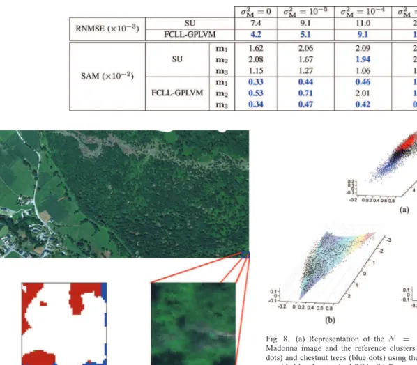
Fig. 7. Top: real hyperspectral Madonna data acquired by the Hyspex hyper-spectral scanner over Villelongue, France. Bottom right: Region of interest shown in true colors (right). Bottom left: ClassiÞcation map obtained in [39] for the region of interest. The labeled pixels are classiÞed as Oak tree (red), Chestnut tree (blue), Ash tree (green) and non-planted-tree pixels (white).
image is considered in this paper to ease the explanation of the results and to keep the processing overhead quite low. This image contains vegetation species of varying spatial density such that some pixels do not contain identiÞed tree species. More precisely, the scene is mainly composed of three com-ponents since the data belong to a two-dimensional manifold (see black dots of Fig. 8(a)). Consequently, we assume that the scene is composed of endmembers.4 We propose to
use the set of 32224 label spectra used in [39] for the learning step of the classiÞcation method presented herein to identify the components present in the area of interest. More precisely, Fig. 8(a) shows the reference clusters corresponding to oak trees (red dots) and chestnut trees (blue dots) projected in a 3-dimen-sional subspace (deÞned by the Þrst three principal components of a PCA applied to the image of Fig. 7). These two clusters are the two closest sets of pixels to vertices of the data cloud. Consequently, oak and chestnut trees are identiÞed as endmem-bers present in the image. Moreover, the new identiÞed end-member is associated with the non-vegetation area (the strategy
4Results of simulations conducted for different values of have been omitted
in this paper for brevity. The results are available in [22].
Fig. 8. (a) Representation of the pixels (black dots) of the Madonna image and the reference clusters corresponding to oak trees (red dots) and chestnut trees (blue dots) using the Þrst three principal components provided by the standard PCA. (b) Representation of the pixels (dots) of the Madonna data and manifold identiÞed by the LL-GPLVM (colored surface). (c) Representation of the pixels (dots) of the Madonna data and boundaries of the estimated transformed simplex (blue lines).
conducted in [39] was restricted to vegetation species). In the sequel, this endmember will be referred to as Endmember .
The simulation parameters have been Þxed to
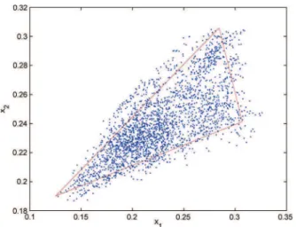
and . The latent variables obtained by maximizing the marginalized posterior distribution (10) are depicted in Fig. 9 (blue dots). It can be seen from this Þgure that the latent variables seem to describe a noisy simplex. Fig. 8(b) shows the manifold estimated by the proposed LL-GPLVM. This Þgure illustrates the capacity of the LL-GPLVM for modeling the nonlinear manifold. Table VI (left) compares the AREs obtained by the proposed LL-GPLVM and the projection onto the Þrst principal vectors provided by PCA. The proposed LL-GPLVM slightly outperforms PCA for the real data of interest, which shows that the proposed nonlinear dimensionality reduction method is more accurate than PCA (linear dimensionality reduction) in representing the data. The scaling step presented in Section IV is then applied to the estimated latent variables. The estimated simplex deÞned by the latent variables is depicted in Fig. 9 (red lines). Fig. 8 (c) compares the boundaries of the estimated transformed simplex with the image pixels. The abundance maps obtained after the scaling step are shown in Fig. 10 (top). The results of the unmixing procedure using the FCLL-GPLVM are compared
Fig. 9. Representation of the latent variables (dots) estimated by the LL-GPLVM and the simplex identiÞed by the scaling step (red lines) for the Madonna data.
TABLE VI ARES: REALIMAGE
Fig. 10. Top: Abundance maps estimated using the FCLL-GPLVM for the Madonna image. Bottom: Abundance maps estimated using the VCA algorithm for endmember extraction and the FCLS algorithm for abundance estimation.
to an unmixing strategy assuming the LMM. More precisely, we use VCA to extract the endmembers from the data and use the FLCS algorithm for abundance estimation. The estimated abundance maps are depicted in Fig. 10 (bottom). The abun-dance maps obtained by the two methods are similar which shows the accuracy of the LMM as a Þrst order approximation of the mixing model. However, the proposed unmixing strategy provides information about the nonlinearly mixed pixels in the image.
Moreover, Fig. 7 (bottom left) shows the classiÞcation map obtained in [39] for the region of interest. The white pixels cor-respond to areas where the classiÞcation method of [39] has not been performed. Since the aim of the work presented in [39] was to locate tree species, a non-planted-tree reference mask was used in [39] to classify only planted-tree pixels. Even if lots of pixels are not classiÞed, the classiÞed pixels can be com-pared with the estimated abundance maps. First, we can note the presence of the same tree species in the classiÞcation and abundance maps, i.e., oak and chestnut. We can also see that
the pixels composed of chestnut trees and Endmember are mainly located in the unclassiÞed regions, which explains why they do not appear clearly in the classiÞcation map. Only one pixel is classiÞed as being composed of ash trees in the region of interest. If unclassiÞed pixels also contain ash trees, they are either too few or too mixed to be considered as mixtures of an additional endmember in the image.
Evaluating the performance of endmember estimation on real data is an interesting problem. However, comparison of the esti-mated endmembers with the ground truth is difÞcult here. First, since the nature of Endmember is unknown, no ground truth is available for this endmember. Second, because of the vari-ability of the ground truth spectra associated with each tree species, it is difÞcult to show whether VCA or the proposed FCLL-GPLVM provides the best endmember estimates. How-ever, the AREs obtained for both methods (Table VI, right) show that the FCLL-GPLVM Þts the data better than the linear SU strategy, which conÞrms the importance of the proposed algo-rithm for nonlinear spectral unmixing.
VIII. CONCLUSIONS
We proposed a new algorithm for nonlinear spectral un-mixing based on a Gaussian process latent variable model. The unmixing procedure assumed a nonlinear mapping from the abundance space to the observed pixels. It also considered the physical constraints for the abundance vectors. The abundance estimation was decomposed into two steps. Dimensionality reduction was Þrst achieved using latent variables. A scaling procedure was then proposed to estimate the abundances. After estimating the abundance vectors of the image, a new endmember estimator based on Gaussian process regression was investigated. This decomposition of the unmixing proce-dure, consisting of Þrst estimating the abundance vectors and subsequently the endmembers, breaks the usual paradigm of spectral unmixing. Simulations conducted on synthetic data illustrated the ßexibility of the proposed model for linear and nonlinear spectral unmixing and provided promising results for abundance and endmember estimations even when there are few pure pixels in the image. It was shown in this paper that the proposed unmixing procedure provides better or com-parable performance (in terms of abundance and endmember estimation) than state of the art unmixing strategies assuming speciÞc mixing models. The choice of the nonlinear mapping used for the GP model is an important issue to ensure that the LL-GPLVM is general enough to handle different nonlin-earities. In particular, different mappings could be used for intimate mixtures. In this paper, the number of endmembers was assumed to be known, which is not true in most practical applications. We think that estimating the number of compo-nents present in the image is an important issue that should be considered in future works. Finally, considering endmember variability in linear and nonlinear mixing models is an inter-esting prospect which is currently under investigation.
ACKNOWLEDGMENT
The authors would like to thank Dr. M. Fauvel from the Uni-versity of Toulouse—INP/ENSAT, Toulouse, France, for sup-plying the real image, reference data, and classiÞcation map re-lated to the classiÞcation algorithm studied in [39] and used in this paper.
REFERENCES
[1] J. M. Bioucas-Dias, A. Plaza, N. Dobigeon, M. Parente, Q. Du, P. Gader, and J. Chanussot, “Hyperspectral unmixing overview: Geomet-rical, statistical, and sparse regression-based approaches,” IEEE J. Sel.
Topics Appl. Earth Observat. Remote Sens., vol. 5, no. 2, pp. 354–379,
April 2012.
[2] N. Keshava and J. F. Mustard, “Spectral unmixing,” IEEE Signal
Process. Mag., vol. 19, no. 1, pp. 44–57, Jan. 2002.
[3] J. Plaza, E. M. Hendrix, I. Garía, G. Martín, and A. Plaza, “On end-member identiÞcation in hyperspectral images without pure pixels: A comparison of algorithms,” J. Math. Imag. Vis., vol. 42, no. 2–3, pp. 163–175, Feb. 2012.
[4] B. Somers, M. Zortea, A. Plaza, and G. Asner, “Automated extraction of image-based endmember bundles for improved spectral unmixing,”
IEEE J. Sel. Topics Appl. Earth Observat. Remote Sens., vol. 5, no. 2,
pp. 396–408, Apr. 2012.
[5] W. Fan, B. Hu, J. Miller, and M. Li, “Comparative study between a new nonlinear model and common linear model for analysing laboratory simulated-forest hyperspectral data,” Remote Sens. Environ., vol. 30, no. 11, pp. 2951–2962, June 2009.
[6] I. Meganem, P. Deliot, X. Briottet, Y. Deville, and S. Hosseini, “Phys-ical modelling and non-linear unmixing method for urban hyperspec-tral images,” in Proc. IEEE GRSS Workshop on Hyperspechyperspec-tral Image
Signal Process., Evolut. Remote Sens. (WHISPERS), Jun. 2011, pp.
1–4.
[7] B. Somers, K. Cools, S. Delalieux, J. Stuckens, D. V. der Zande, W. W. Verstraeten, and P. Coppin, “Nonlinear hyperspectral mixture analysis for tree cover estimates in orchards,” Remote Sens. Environ., vol. 113, no. 6, pp. 1183–1193, 2009.
[8] J. M. P. Nascimento and J. M. Bioucas-Dias, “Nonlinear mixture model for hyperspectral unmixing,” in Proc. SPIE, 2009, vol. 7477, pp. 74 770I–74 770I-8.
[9] A. Halimi, Y. Altmann, N. Dobigeon, and J.-Y. Tourneret, “Nonlinear unmixing of hyperspectral images using a generalized bilinear model,”
IEEE Trans. Geosci. Remote Sens., vol. 49, no. 11, pp. 4153–4162,
Nov. 2011.
[10] B. W. Hapke, “Bidirectional reßectance spectroscopy. I. Theory,” J.
Geophys. Res., vol. 86, pp. 3039–3054, 1981.
[11] K. J. Guilfoyle, M. L. Althouse, and C.-I. Chang, “A quantitative and comparative analysis of linear and nonlinear spectral mixture models using radial basis function neural networks,” IEEE Geosci. Remote
Sens. Lett., vol. 39, no. 8, pp. 2314–2318, Aug. 2001.
[12] Y. Altmann, N. Dobigeon, S. McLaughlin, and J.-Y. Tourneret, “Non-linear unmixing of hyperspectral images using radial basis functions and orthogonal least squares,” in Proc. IEEE Int. Conf. Geosci.
Re-mote Sens. (IGARSS), July 2011, pp. 1151–1154.
[13] Y. Altmann, A. Halimi, N. Dobigeon, and J.-Y. Tourneret, “Supervised nonlinear spectral unmixing using a postnonlinear mixing model for hyperspectral imagery,” IEEE Trans. Image Process., vol. 21, no. 6, pp. 3017–3025, 2012.
[14] J. Broadwater, R. Chellappa, A. Banerjee, and P. Burlina, “Kernel fully constrained least squares abundance estimates,” in Proc. IEEE
Int. Conf. Geosci. Remote Sens. (IGARSS), July 2007, pp. 4041–4044.
[15] K.-H. Liu, E. Wong, and C.-I. Chang, “Kernel-based linear spectral mixture analysis for hyperspectral image classiÞcation,” in Proc. IEEE
GRSS Workshop Hyperspectral Image Signal Process., Evolut. Remote Sens. (WHISPERS), Aug. 2009, pp. 1–4.
[16] J. Chen, C. Richard, and P. Honeine, “A novel kernel-based nonlinear unmixing scheme of hyperspectral images,” in Proc. Asilomar Conf.
Signals, Syst., Comput., Nov. 2011, pp. 1898–1902.
[17] J. Chen, C. Richard, and P. Honeine, “Nonlinear unmixing of hyper-spectral data based on a linear-mixture/nonlinear-ßuctuation model,”
IEEE Trans. Signal Process., vol. 61, no. 2, pp. 480–492, 2013.
[18] R. Heylen, D. Burazerovic, and P. Scheunders, “Non-linear spectral unmixing by geodesic simplex volume maximization,” IEEE J. Sel.
Topics Signal Process., vol. 5, no. 3, pp. 534–542, Jun. 2011.
[19] N. D. Lawrence, “Gaussian process latent variable models for visual-isation of high dimensional data,” in Proc. NIPS, Vancouver, Canada, 2003.
[20] E. V. Bonilla, F. V. Agakov, and C. K. I. Williams, “Kernel multi-task learning using task-speciÞc features,” J. Mach. Learning Res.- Proc.
Tracks, pp. 43–50, 2007.
[21] M. A. Alvarez, L. Rosasco, and N. D. Lawrence, “Kernels for vector-valued functions: A review,” Jun. 2011 [Online]. Available: http://arxiv.org/abs/1106.6251
[22] Y. Altmann, N. Dobigeon, S. McLaughlin, and J.-Y. Tourneret, “Non-linear spectral unmixing of hyperspectral images using Gaussian pro-cesses,” Univ. of Toulouse, Toulouse, France, Tech. Rep., Nov. 2012 [Online]. Available: http://altmann.perso.enseeiht.fr/
[23] J. Quionero-candela, C. E. Rasmussen, and R. Herbrich, “A unifying view of sparse approximate Gaussian process regression,” J. Mach.
Learn. Res., vol. 6, p. 2005, 2005.
[24] N. D. Lawrence, “The Gaussian process latent variable model,” Comput. Sci. Dept., Univ. of ShefÞeld, Tech. Rep., Jan. 2006 [Online]. Available: http://staffwww.dcs.shef.ac.uk/people/N.Lawrence/ [25] J. Wang and C.-I. Chang, “Applications of independent component
analysis in endmember extraction and abundance quantiÞcation for hy-perspectral imagery,” IEEE Trans. Geosci. Remote Sens., vol. 4, no. 9, pp. 2601–2616, Sep. 2006.
[26] R. Urtasun, D. J. Fleet, and N. D. Lawrence, “Modeling human lo-comotion with topologically constrained latent variable models,,” in
Proc. Conf. Human Motion, Understand., Model., Capture, Animat.,
Rio de Janeiro, Brazil, 2007, pp. 104–118.
[27] C. E. Rasmussen and C. K. I. Williams, Gaussian Processes
for Machine Learning (Adaptive Computation and Machine Learning). Cambridge, MA, USA: MIT Press, 2005.
[28] M. Brookes, The Matrix Reference Manual. London, U.K.: Imperial College, 2005.
[29] N. Dobigeon, S. Moussaoui, M. Coulon, J.-Y. Tourneret, and A. O. Hero, “Joint Bayesian endmember extraction and linear unmixing for hyperspectral imagery,” IEEE Trans. Signal Process., vol. 57, no. 11, pp. 2657–2669, Nov. 2009.
[30] F. Chaudhry, C.-C. Wu, W. Liu, C.-I. Chang, and A. Plaza, “Pixel pu-rity index-based algorithms for endmember extraction from hyperspec-tral imagery,” in Recent Advances in Hyperspechyperspec-tral Signal and Image
Processing, C.-I. Chang, Ed. Trivandrum, Kerala, India: Research Signpost, 2006, ch. 2.
[31] M. Winter, “Fast autonomous spectral end-member determination in hyperspectral data,” in Proc. 13th Int. Conf. Appl. Geologic Remote
Sens., Vancouver, Canada, Apr. 1999, vol. 2, pp. 337–344.
[32] J. M. P. Nascimento and J. M. Bioucas-Dias, “Vertex component analysis: A fast algorithm to unmix hyperspectral data,” IEEE Trans.
Geosci. Remote Sens., vol. 43, no. 4, pp. 898–910, Apr. 2005.
[33] J. Li and J. M. Bioucas-Dias, “Minimum volume simplex analysis: A fast algorithm to unmix hyperspectral data,” in Proc. IEEE Int. Conf.
Geosci. Remote Sens. (IGARSS), Boston, MA, USA, Jul. 2008, vol. 3,
pp. 250–253.
[34] “ENVI User’s Guide,” ver. 4.0, RSI (Research Systems Inc.), Boulder, CO, USA, Sep. 2003, 80301.
[35] D. C. Heinz and C.-I. Chang, “Fully constrained least-squares linear spectral mixture analysis method for material quantiÞcation in hyper-spectral imagery,” IEEE Trans. Geosci. Remote Sens., vol. 29, no. 3, pp. 529–545, Mar. 2001.
[36] O. Eches, N. Dobigeon, C. Mailhes, and J.-Y. Tourneret, “Bayesian estimation of linear mixtures using the normal compositional model,”
IEEE Trans. Image Process., vol. 19, no. 6, pp. 1403–1413, Jun. 2010.
[37] B. Somers, G. P. Asner, L. Tits, and P. Coppin, “Endmember variability in spectral mixture analysis: A review,” Remote Sens. Environ., vol. 115, no. 7, pp. 1603–1616, 2011.
[38] A. Zare, P. Gader, T. Allgire, D. Drashnikov, and R. Close, “Boot-strapping for piece-wise convex endmember distribution detection,” in Proc. IEEE GRSS Workshop Hyperspectral Image SIgnal Process.,
Evolut. Remote Sens. (WHISPERS), May 2012, pp. 1–4.
[39] D. Sheeren, M. Fauvel, S. Ladet, A. Jacquin, G. Bertoni, and A. Gibon, “Mapping ash tree colonization in an agricultural mountain landscape: Investigating the potential of hyperspectral imagery,” in Proc. IEEE
Int. Conf. Geosci. Remote Sens. (IGARSS), Jul. 2011, pp. 3672–3675.
Yoann Altmann (S’10) was born in Toulouse,
France, in 1987. He received the Eng. degree in elec-trical engineering from the ENSEEIHT, Toulouse, France, and the M.Sc. degree in signal processing from the National Polytechnic Institute of Toulouse, Toulouse, France, both in 2010.
He is currently working towards the Ph.D. degree with the Signal and Communication Group, IRIT Laboratory, Toulouse, France.
Nicolas Dobigeon (S’05–M’08) was born in
An-goulême, France, in 1981. He received the Eng. degree in electrical engineering from ENSEEIHT, Toulouse, France, the M.Sc. degree in signal pro-cessing from the National Polytechnic Institute of Toulouse (INP Toulouse), France, both in 2004, and the Ph.D. degree and Habilitation à Diriger des Recherches degree in signal processing from the INP Toulouse in 2007 and 2012, respectively.
From 2007 to 2008, he was a Postdoctoral Re-search Associate with the Department of Electrical Engineering and Computer Science, University of Michigan, Ann Arbor, MI, USA. Since 2008, he has been with the National Polytechnic Institute of Toulouse (INP-ENSEEIHT, University of Toulouse), where he is currently an Associate Professor. He conducts his research within the Signal and Communications Group of the IRIT Laboratory, and he is also an afÞliated faculty member of the Telecommunications for Space and Aeronautics (TeSA) cooperative laboratory. His recent research activities have been focused on statistical signal and image processing, with a particular interest in Bayesian inverse problems with applications to remote sensing, biomedical imaging, and genomics.
Steve McLaughlin (F’11) was born in Clydebank,
Scotland, U.K., in 1960. He received the B.Sc. de-gree in electronics and electrical engineering from the University of Glasgow, Scotland, U.K., in 1981 and the Ph.D. degree from the University of Edinburgh, Scotland, U.K., in 1990.
From 1981 to 1984, he was a Development Engi-neer in the industry, involved in the design and simu-lation of integrated thermal imaging and Þre control systems. From 1984 to 1986, he worked on the design and development of high-frequency data communi-cation systems. In 1986, he joined the Department of Electronics and Electrical Engineering at the University of Edinburgh as a Research Fellow, where he
studied the performance of linear adaptive algorithms in high noise and non-stationary environments. In 1988, he joined the academic staff at Edinburgh, and from 1991 until 2001, he held a Royal Society University Research Fellow-ship to study nonlinear signal processing techniques. In 2002, he was awarded a personal Chair in Electronic Communication Systems at the University of Edin-burgh. In October 2011, he joined Heriot-Watt University, Edinburgh, U.K., as a Professor of Signal Processing and Head of the School of Engineering and Phys-ical Sciences. His research interests lie in the Þelds of adaptive signal processing and nonlinear dynamical systems theory and their applications to biomedical, energy, and communication systems.
Prof. McLaughlin is a Fellow of the Royal Academy of Engineering, the Royal Society of Edinburgh, and the Institute of Engineering and Technology.
Jean-Yves Tourneret (SM’08) received the
In-génieur degree in electrical engineering from the École Nationale Supérieure d’Électronique, d Électrotechnique, dInformatique, dHydraulique, et des Télécommunications (ENSEEIHT), Toulouse, France, in 1989 and the Ph.D. degree from National Polytechnic Institute, Toulouse, France, in 1992.
He is currently a Professor with ENSEEIHT and a Member of the IRIT Laboratory (UMR 5505 of the CNRS). His current research interests include statis-tical signal processing with a particular interest to Bayesian methods and Markov chain Monte Carlo (MCMC) algorithms.
Prof. Tourneret was the Program Chair of the European Conference on Signal Processing (EUSIPCO), held in Toulouse, France, in 2002. He was also a member of the Organizing Committee for the International Conference of Acoustics, Speech and Signal Processing (ICASSP) in Toulouse, France, in 2006. He has been a member of different technical committees, including the Signal Processing Theory and Methods (SPTM) Committee of the IEEE Signal Processing Society from 2001 to 2007 and 2010 to present. He has been serving as an Associate Editor for the IEEE TRANSACTIONS ONSIGNALPROCESSING