HAL Id: hal-00316990
https://hal.archives-ouvertes.fr/hal-00316990
Submitted on 1 Jan 2003
HAL is a multi-disciplinary open access
archive for the deposit and dissemination of
sci-entific research documents, whether they are
pub-lished or not. The documents may come from
teaching and research institutions in France or
abroad, or from public or private research centers.
L’archive ouverte pluridisciplinaire HAL, est
destinée au dépôt et à la diffusion de documents
scientifiques de niveau recherche, publiés ou non,
émanant des établissements d’enseignement et de
recherche français ou étrangers, des laboratoires
publics ou privés.
energetic electron plasma
D. Nunn, A. Demekhov, V. Trakhtengerts, M. J. Rycroft
To cite this version:
D. Nunn, A. Demekhov, V. Trakhtengerts, M. J. Rycroft. VLF emission triggering by a highly
anisotropic energetic electron plasma. Annales Geophysicae, European Geosciences Union, 2003, 21
(2), pp.481-492. �hal-00316990�
Annales
Geophysicae
VLF emission triggering by a highly anisotropic energetic electron
plasma
D. Nunn1, A. Demekhov2, V. Trakhtengerts2, and M. J. Rycroft3
1Dept of Electronics and Computer Science, Southampton University, Southampton ,Hants SO17 1BJ, UK 2Institute of Applied Physics, 46 Ulyanov St., Nizhni Novgorod 603600, Russia
3CAESAR Consultancy , 35 Millington Rd, Cambridge CB3 9HW, UK and Faculty of Computing and Engineering Sciences,
De Montfort University, Leicester LE1 9BH, UK
Received: 28 January 2002 – Revised: 1 October 2002 – Accepted: 21 October 2002
Abstract. A recent paper (Bell et al., 2000) reports
observa-tions from the POLAR spacecraft of highly anisotropic hot electron distribution functions in the equatorial region of the magnetosphere at L = 3.4. The particle instrument HY-DRA measures electron fluxes from 1–20 keV. VLF emis-sions triggered by pulses from Omega (Norway) are found to coincide with “pancake” type electron distributions with average pitch angles >70 degrees, such distributions being effectively confined to the equatorial zone. We examine the linear and nonlinear wave particle interaction process be-tween pancake distributions and continuous wave (CW) or narrow band ducted whistler mode signals. It is concluded that the pitch angle range of 67–76 degrees dominates the in-teraction process, and that with in-duct wave saturation am-plitudes of 6 pT strong nonlinear trapping occurs for these particles. Using these data, a 1-D Vlasov Hybrid Simulation VLF code was run to simulate numerically risers triggered by a 1 s Omega pulse. The integrated linear trans-equatorial amplification of ∼15 dB agrees well with figures calculated by Bell et al. (2000) from the HYDRA data. Fallers, hooks and oscillating tones have also been simulated.
Key words. Space plasma physics (numerical simulation
studies; wave particle interactions) Solar physics, astro-physics and astronomy (radio emission)
1 Introduction
The phenomenon of triggered VLF radio (whistler mode) emissions is a very important theoretical problem in space plasma physics. It is a “clean”, reproducible and highly non-linear phenomenon. Furthermore, a wealth of supporting ex-perimental data has been produced by the active Siple exper-iment in Antarctica (Helliwell and Katsufrakis, 1974; Helli-well et al., 1980, 1986; HelliHelli-well, 1983), enabling a detailed comparison to be made between theory and simulations, on the one hand, and real data on the other.
Correspondence to: D. Nunn ([email protected])
In recent years, many papers have been written on the the-ory and simulation of triggered VLF emissions (Helliwell, 1967; Helliwell and Inan, 1982; Molvig et al., 1988; Roux and Pellat, 1978; Sa, 1990; Trakhtengerts et al., 1996; Nunn, 1986, 1990; Carlson, 1990). Space prohibits an adequate re-view; a useful overview of competing theories is found in Omura et al. (1991), but this review is now in need of up-dating. There seems to be reasonable agreement that the driving mechanism is the nonlinear cyclotron resonance be-tween narrow band/band limited ducted VLF waves propa-gating along a geomagnetic field line and energetic keV elec-trons. Particle trajectory nonlinearity is synonymous with the well-known concept of phase trapping (Nunn, 1990). The parabolic inhomogeneity imposed by the ambient magnetic field variation confines the significant interaction region to within a few thousand kms of the equator, and profoundly controls the detailed trapping dynamics of the wave particle interaction process.
In view of the nonlinearity and complexity of the prob-lem, the main avenue of recent research has been numerical simulation. Particle-in-cell simulations have provided use-ful results (Helliwell and Crystal, 1973; Carlson et al., 1990; Omura and Matsumoto, 1982), but more recent computations have used the Vlasov Hybrid Simulation (VHS) technique (Nunn, 1990, 1993, 1997). It is well known that Vlasov sim-ulation techniques are extremely efficient and effective for the numerical simulation of plasma, particularly with prob-lems with one spatial dimension (Cheng and Knorr, 1976; Denavit, 1972; Chanteur, 1985). VHS simulations have pro-duced triggered emissions and resulted in the production of self sustaining “generating regions” that cause sweeping fre-quencies as observed. In fact, risers, fallers and hooks have all been modelled (Smith et al., 1998). It should be noted though that quite a few aspects of experimental reality re-main poorly described by these codes, in particular the slow exponential growth phase at low amplitudes observed with Siple key down signals (Helliwell, 1983) and the absence of an adequate plasma physical description of the amplitude sat-uration mechanism operating (Nunn et al., 1997, 1999).
A difficulty facing simulationists is the absence to date of experimental wave and particle observations actually at the site of the wave particle interactions, presumably inside a narrow duct of enhanced plasma density in the equato-rial zone. The simulations of Nunn (Nunn, 1993) tended to use (for the Siple case) maximum wave amplitudes ∼3–6 pT, some 2–3 times larger than the amplitudes at which nonlin-ear trapping of electrons by the wave commences. Ambient distribution functions were of the high flux, low anisotropy type, with typical equatorial linear growth rates ∼70 dB/s. Electrons contributing the most power to the wave field were in the pitch angle range of 40–60 degrees. Working in this re-gion of “parameter” space gave “good” emissions, but these tended to be fairly explosive, corresponding to a nonlinear absolute instability. Almost any signal injected into the sim-ulation box resulted in a triggered emission. The question that has to be asked is: are we working in the correct region in parameter space?
A recent important paper (Bell et al., 2000) provides valu-able observations of equatorial electron distribution func-tions in the energy range 1–20 keV at an L-shell of 3.4. Very high electron anisotropies were found to coincide with the triggering of VLF emissions by 1 s pulses from the Omega Norway transmitter. These observations have considerable significance for the theory and numerical modelling of trig-gered VLF emissions. In this paper we take the distribution function used by Bell et al. (2000) to model the observed electron data, and examine the implications for wave particle interaction processes and particularly for nonlinear trapping. A full numerical simulation of Omega pulse triggering, again using the distribution function of Bell et al. (2000), follows.
2 The wave and particle observations from the POLAR spacecraft
The particle and wave data reported by Bell et al. (2000) were obtained from the POLAR spacecraft, with the PWI instrument furnishing the VLF wave data (Gurnett et al., 1995) and the HYDRA instrument furnishing the particle data (Scudder et al., 1995). The data presented were from the equatorial region at L = 3.4 + −0.1 on 13 January 1997, though these data were typical of the entire data set gath-ered during 1996/1997. The HYDRA instrument measures energetic electron fluxes in the energy range 1–20 keV. Bell et al. (2000) found that the perpendicular fluxes J⊥(in the
pitch angle range α = 75 − 105◦) were greater than the
par-allel fluxes Jk(α = 0− > 30◦)by a factor of typically 14.
Furthermore, J⊥decreased abruptly at geomagnetic latitudes
of ±15◦, indicating a “pancake” type distribution with a pre-ponderance of very high pitch angle (>70 degrees) particles. Simultaneously with these particle observations the plasma wave instrument PWI observed triggering activity by 1 s du-ration Omega (Norway) pulses on 10.2 kHz. According to the ray tracing analysis in Bell et al. (2000), to which the reader is referred, evidence is presented that the spacecraft actually observed unducted signals backscattered from the
duct termination: because of this the spectrograms were a good deal less clear than those obtained from ground obser-vations of ducted signals.
Based mainly on the observed latitude dependence of en-ergetic electron fluxes, Bell et al. (2000) have produced an analytic model distribution function Foto fit the observations
of electron differential fluxes as a function of magnetic lati-tude, which is of the form
Fo(µ, W ) = cW−2(µ/W )12.5, (1)
where µ is the magnetic moment and W is the dimensionless energy. The exponent of 12.5 shown, however, does not ap-pear to be consistent with the observed ratios of J⊥/Jk∼14,
and would require values for this ratio ∼ 107. For the HY-DRA data, and using this model, at L = 3.4 the integrated trans-equatorial amplification at 10.2 kHz was calculated to be ∼7 dB using only electrons with energies up to 20 keV, a rather modest figure. This value becomes 14 dB if the above functional form for Fo is assumed to extend to all energies
above 20 keV, which is the upper limit of HYDRA’s mea-surements.
The analytic form above is not necessarily the best fit to the data, as was pointed out by Pasmanik and co-workers (Pas-manik et al., 2001; Trakhtengerts et al., 2001). They demon-strated that step-like discontinuities in the equatorial parallel velocity of the electrons could account for the HYDRA ob-servations. In fact, theory points to the need for more sophis-ticated models, such as the multiple bi-Maxwellian, in which anisotropy is a (decreasing) function of energy. Considering gyro-resonance with Omega transmissions, the electron en-ergy exceeds 20 keV at pitch angles ∼ 79◦. We do not know what the gradients in V⊥/Vk space are at higher pitch
an-gles. Thus, extending the above model to all energies may overestimate the anisotropy.
We should also bear in mind that these results represent one set of observations at a particular L-shell (L = 3.4). It is not clear what anisotropy levels prevail at higher L-shells, particularly for Siple at L = 4.2. Nonetheless, it is clear that these latest observations from Bell et al. (2000) are of con-siderable importance. We now consider the implications for the wave particle interaction process, and endeavour to sim-ulate Omega triggered emissions using distribution functions of this type.
3 Wave particle interaction dynamics
We must now address a number of crucial issues. Using the model “pancake” distribution function of Bell et al. (2000), what is the relative contribution to the linear equatorial cy-clotron growth rate at 10.2 kHz as a function of equatorial pitch angle α? The linear growth rate has a twofold signifi-cance, in that it provides the initial amplification that raises the weak input signals to levels at which nonlinear trapping of electrons by the wave takes place. Second, nonlinear growth rates in a parabolic inhomogeneity, although in prin-ciple functions of space and time, generally have an order
0.95 1 1.05 1.1 1.15 1.2 1.25 1.3 1.35 1.4 1.45 1 2 3 4 5 6 7
Contour plot of distribution function
−Parallel velocity
Perpendicular velocity
Vz=Vres
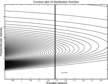
Fig. 1. Contour plot in equatorial Vz, |V ⊥ |space of the
“pan-cake” distribution function of Bell et al. (2000). Velocities are in dimensionless units.
of magnitude equal to the linear growth rate multiplied by a factor equal to the number of trapping oscillations undergone by the resonant particles (Nunn, 1990, 1993).
The following development will henceforth employ di-mensionless units defined as follows. The unit of time is given by
1t =1/ ω = 2/ e(eq),
where e(eq)is the electron gyrofrequency at the equator.
The unit of frequency and also the unit of growth rate is 1f = ω = e(eq)/2.
The unit of length is given by 1z =1/k = c/5eq,
where 5eq is the electron plasma frequency at the equator
and c is the velocity of light. The unit of wave number be-comes
1k = k = 5eq/c.
The unit of velocity is 1v = 1z/1t, and energy and mag-netic moment are referred to W = 1v2. Resonant particle distribution functions are referred to 1F = 1/(1v31x3). The linear cyclotron growth rate at frequency ω0was given
in Nunn (1990) in the following dimensionless form
γlin=c
Z ∞
0
|V ⊥ |3[∂F0/∂W
+(2/ω0)∂F0/∂µ]V z=V resd|V ⊥ |, (2)
where F0(µ, W )is the zero order distribution function as a
function of magnetic moment µ and energy W , and c is a dimensionless constant whose exact expression will not be
10 20 30 40 50 60 70 80 100
101 102 103
Pitch angle degrees
Resonant energy keV
Log plot of resonant energy vs pitch angle
Fig. 2. Dependence of particle energy on pitch angle for electrons cyclotron resonant with Omega pulses.
given here. Following Bell et al. (2000) we assume a zero order distribution function of the form
F0(µ, W ) = cW−n[µ/W ]m.
Here, we take n = 2.5, a little larger (and more realistic) than their Figure of 2, and m = 12.5, corresponding to a very anisotropic “pancake” pitch angle dependence varying as (sin α)25. In fact, the exponent of n = 2 used by Bell et al. (2000) gives the high energy tail of the hot electron distribution infinite kinetic energy, which we deemed to be unrealistic. Other parameters employed are f = 10200 Hz, L = 3.4, cold plasma density Ne =800/cc and electron
gy-rofrequency = 22400 Hz.
Figure 1 shows a contour plot of F0 in the |V ⊥ | ,Vz
plane. Note that γlinis given by integrating the gradient term
|V ⊥ |3F00along the line defined by Vz=Vres=(ω−)/ k
for the Omega signals at f = 10.2 kHz. Figure 2 plots the resonant electron energy as a function of pitch angle for this case; it is seen that the upper energy limit of the HYDRA detector is reached at a pitch angle of 79 degrees. The dis-tribution function at higher pitch angles can only be inferred by extrapolation.
We now compute the cumulative contribution to the linear growth rate as a function of the equatorial pitch angle α. This is given by the expression below, in dimensionless units; it is plotted as the dashed curve in Fig. 4.
γlin(α) = c Z V ⊥(0) 0 |V ⊥ |3[∂F0/∂W +(2/ω0)∂F0/∂µ]Vz=Vresd|V ⊥ |, (3) where V ⊥ (0) = tan(α)|Vres|.
Half the cumulative total is reached at a pitch angle of 72.5 degrees, where the gradient of the curve is maximal. The dominant contributors (80%) to the linear growth rate are
0 10 20 30 40 50 60 70 80 90 0 1 2 3 4 5 6 7 8
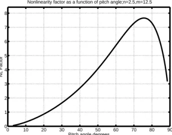
Nonlinearity factor as a function of pitch angle;n=2.5,m=12.5
Pitch angle degrees
NL Factor
Fig. 3. The nonlinearity factor η, as a function of pitch angle. This is approximately equal to the maximum number of trapping oscil-lations of resonant particles in the equatorial zone.
seen to be electrons with pitch angles in the range of α = 62– 82 degrees, with a maximum at 72.5 degrees. This figure is somewhat less than that of 80 degrees implied in Bell et al. (2000), partly because our attention is confined to elec-trons that are gyro-resonant at the frequency of the Omega signal.
It is believed that the process of VLF emission trigger-ing comes about from nonlinear wave particle interactions, since the process itself is clearly highly nonlinear in charac-ter (Nunn, 1990). Resonant particle nonlinearity is synony-mous with particle “phase trapping”, which in a parabolic inhomogeneity was looked at in some detail by Karpman et al. (1974) and Nunn (1990, 1993). We do not repeat all the calculations therein.
Assuming a saturated in-duct wave amplitude of 6 pT, a realistic but required choice, we have calculated the nonlin-earity factor η, which is the (maximum) number of trapping oscillations undergone by resonant particles in the equato-rial zone, within the physical trapping region length L(|V⊥|).
Referring to Nunn (1990, 1993) the dimensionless equations of motion of cyclotron resonant electrons may be written in the form below, assuming a CW pulse of constant amplitude 6 pT
v∗=Vz−Vres(z)
ψ0=kv∗
v∗0 = −Rk0|V⊥|/ω0·cos ψ + Q0(z), (4)
where R is the dimensionless wave amplitude given by R = e|E|k/mω2
and ψ is the phase angle between the perpendicular velocity vector and the wave electric field vector, and Q0(z)is the
ef-fective “force” due to the sum of all inhomogeneities present. This may be written in the form (Nunn, 1990)
Q0(z) = A(|V⊥|)z 40 45 50 55 60 65 70 75 80 85 90 0 0.1 0.2 0.3 0.4 0.5 0.6 0.7 0.8 0.9 1
Accumulated contribution to linear/nonlinear growth;n=2.5,m=12.5
Pitch angle degrees
NL Growth
Fig. 4. Accumulated fractional contribution to the linear equatorial growth rate (dashed curve) and nonlinear growth rate (solid curve) at f = 10.2 kHz, for the high anistropy “pancake” distribution. The nonlinear contribution is weighted by the size of the nonlinear trapping region.
A(|V⊥| = [χ (3Vres/ k0− |V⊥|2/2β) + νzVres2 /2γe], (5)
where Vres(z) = (ω0−2β)/ k0is the local cyclotron
reso-nance velocity, β(z) is the ambient magnetic field strength relative to that at the equator, and is assumed to have a parabolic dependence on z
β =1 + 0.5χ z2=B(z)/B(0)
and γ (z) is the corresponding quantity for cold electron den-sity
γe =1 + 0.5νχ z2=Ne(z)/Ne(0),
where ν = 0.5 throughout. From the equations of motion it is seen that the condition for just trapping is satisfied at Zt r,
where
Rk0|V⊥|/ω0=A(|V⊥|)Zt r
and hence the maximum possible trapping length L for a par-ticle of a specified perpendicular velocity is as below, where we are making the assumption that the wave field is constant L(|V⊥|) =2Zt r =2Rk0|V ⊥ |/(A(|V⊥|)ω0).
The nonlinearity factor η is defined as the maximum number of whole trapping oscillations that an electron may undergo in the equatorial zone, and is given by
η(|V⊥|) = L(|V ⊥ |)ωt r/2π,
where ωt r is the angular trapping frequency. For simplicity
we use the expression derived at the equator which is ωt r=
q
Rk02|V⊥|/ω0.
Nonlinearity factor η is plotted in Fig. 3, as a function of pitch angle. In a parabolic inhomogeneity, the trapping dy-namics are very complex, as the trap geometry is constantly
changing, and the above calculation is somewhat simplified. It is seen that the strongest nonlinearity occurs at a pitch gle of 75 degrees and falls off steadily at higher pitch an-gles. It was shown (Nunn, 1990) that the nonlinear trapping time goes as |V⊥|−0.5. The inhomogeneity factor S contains
a term in z|V⊥|. The point where phase trapping is first
per-mitted is where S = −1 and hence the width of the perper-mitted zone for trapping, L(|V⊥|)goes as |V⊥|−1.0at high pitch
an-gles.
The key question now is what is the relative contribution to the nonlinear growth rate as a function of pitch angle? Again, the nonlinear growth rate is purely local in space and time, but its order of magnitude is estimated by:
γnonlin∼η γlin.
We have estimated the cumulative contribution to the nonlin-ear growth rate through the expression
γnonlin(α) = c Z V⊥(0) 0 |V ⊥ |3η(|V ⊥ |) h ∂F0/∂W + (2/ω0)∂F0/∂µ i VzVres Ld|V ⊥ |, (6) where V ⊥ (0) = tan(α)|Vres|.
It should be noted that in reality the nonlinear growth rate is a function of space and time, and will be properly cal-culated in the simulation code. The above expression is a rough estimation of the size of the nonlinear growth rate and the relative contributions from electrons of different pitch an-gles. We have further weighted the contribution to the non-linear growth by the quantity L(|V⊥|), which is the size of
the nonlinear interaction region along the geomagnetic field line that becomes very small at extremely high pitch angles. The result is plotted as the solid curve in Fig. 4, and shows a maximum contribution from pitch angles of 72 degrees. The overwhelming contribution (80%) comes from the range be-tween 63–79 degrees. The curves for the accumulated contri-bution to the growth rate are actually very close in the linear and nonlinear cases, with the nonlinear case being shifted to-wards lower pitch angles.
Since the saturation in-duct amplitude has not yet been measured directly, it is important to ask: with the Bell et al. (2000) distribution, at what wave amplitude does nonlin-earity set in? We estimate this by assuming that trapping commences when the nonlinearity factor exceeds unity at some pitch angle. Some numerical experiments showed that this is close to 2 pT. Thus, for the pancake distribution func-tion the nonlinear theory of triggered Omega VLF emissions requires in-duct amplitudes to exceed 2 pT. This requirement must not be confused with the input amplitudes of the signals from the transmitter, which are of course small, ∼0.1 pT. The input signal is subject to considerable linear and nonlinear amplification during propagation to the equator, and further-more, in the nonlinear zone, the nonlinear growth rates can be very large (∼300 dB/s). 40 45 50 55 60 65 70 75 80 85 90 0 0.1 0.2 0.3 0.4 0.5 0.6 0.7 0.8 0.9 1
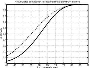
Accumulated contribution to linear/nonlinear growth;n=2.5,m=3
Pitch angle degrees
NL Growth
Fig. 5. Accumulated fractional linear and nonlinear growth rates, as functions of pitch angle for a low anisotropy distribution function
n =2.5, m = 3.
By way of comparison it is useful to consider a distribu-tion funcdistribu-tion with a more modest anisotropy, namely with n = 2.5, m = 3. Figure 5 shows the accumulated contri-bution to linear and nonlinear growth rates as a function of pitch angle for this case. In the linear case (dashed curve) the maximum contribution comes from pitch angles ∼55 de-grees, with the range of 40–71 degrees accounting for 80% of the power input. In the nonlinear case (solid curve) the con-tribution peaks at a higher pitch angle of 61 degrees, with the range from 46–73 degrees accounting for 80% of the power input. Experimentation with the simulation showed that, in this case, nonlinear trapping commences at wave amplitudes ∼1.6 pT.
It is clear that highly anisotropic pitch angle distributions do not radically alter the nature of resonant particle dynam-ics. Use of a Bell et al. (2000) type distribution function has raised the pitch angle of maximum nonlinear contribu-tion from 61 to 72 degrees, and reduced the particle nonlin-earity somewhat, in that the onset of trapping occurs at 2 pT rather than 1.6 pT. It seems that the in-duct wave amplitudes and the overall energetic electron fluxes are more important than the values of the anisotropy levels.
4 Numerical modelling of Omega triggered VLF emis-sions
We have established that, even with highly anisotropic en-ergetic electron distribution functions of the kind described by Bell et al. (2000), nonlinear trapping of cyclotron reso-nant electrons will be the domireso-nant feature of the wave par-ticle interaction process and the root cause of triggered VLF emissions. Such excellent particle and wave data are an op-portunity to put theory and simulation to the test. A logi-cal progression is now to undertake a full numerilogi-cal mod-elling of VLF emissions triggered by Omega pulses, using
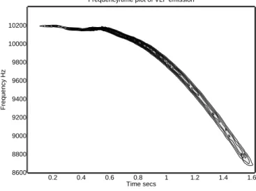
0.2 0.4 0.6 0.8 1 1.2 1.4 1.6 1.8 2 2.2 1 1.02 1.04 1.06 1.08 1.1 1.12 1.14 1.16 1.18 1.2 x 10⁴ Time secs Frequency Hz
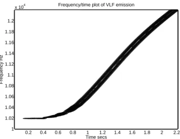
Frequency/time plot of VLF emission
Fig. 6. Run 1. Omega triggered riser. Frequency time spectrogram of the wave field data stream exiting from the interaction region. Actual numerical values are arbitrary.
the zero order distribution functions as described by Bell et al. (2000). We have used the highly anistropic model of Bell et al. (2000), based on the latitudinal dependence of electron fluxes. A model based on the ratio J⊥/Jk∼14 would have a
lower anistropy, but the main conclusions of this paper would apply in equal measure to cases of intermediate anisotropy.
The simulation code used is a 1-D Vlasov Hybrid Simu-lation code (VHS/VLF) whose methodology has been fully described in the literature (Nunn, 1990, 1993). A phase space simulation box is defined in a 4-dimensional space {z, V∗, |V ⊥ |,and ψ }. The coordinate z is the curvilinear distance from the equator along the ambient magnetic field line and covers a region of about 3000 km on either side of the equator, which is where nonlinear trapping occurs. The quantity ψ is the phase of the perpendicular velocity |V ⊥ | relative to the wave electric field, while V∗ = Vz −Vres
is the parallel velocity relative to the local initial cyclotron resonance velocity Vres. The phase box occupies a range
of V∗ equal to about 3 trapping widths plus the range of
resonant velocity appertaining to the simulation bandwidth. Since triggered emissions have sweeping frequencies, it is imperative that the phase box moves in V∗to track the local resonant region in z and t, and thus to resolve the nonlinear resonant particle dynamics at all times.
In the present problem a z grid of 2048 points is used, more than sufficient to resolve the spatial structure of the genera-tion region. The simulagenera-tion time-step is 1t = 1z/|Vres|,
which is small enough to integrate resonant electron trajecto-ries accurately. The number of grid points in V∗is NV∗=40
and in 9 is N9 = 16. The coordinate |V ⊥ | is relatively
“weak” in that only a few grid points are needed. We shall use a value NV ⊥ = 3 throughout. The unperturbed
distri-bution function taken is the “pancake” distridistri-bution of Eq. 1. We have reverted to n = 2, which is justified as the simula-tion only employs electrons with energy up to ∼20 keV. The
|V ⊥ | grid values will correspond to pitch angles of 66◦,
71◦and 77◦, which are the 25%, 50% and 75% values for
the integrated contribution to the nonlinear growth rates as shown in Fig. 4. At each time step the wave field is band-pass-filtered to a bandwidth of ∼20 to 40 Hz, somewhat less than the maximum trapping frequency ∼70 Hz here. When wider bandwidths of the order of the trapping frequency or greater are used, sidebands develop, causing detrapping of resonant electrons, reducing the degree of particle nonlin-earity and growth rates. Numerical experimentation showed that broad bandwidths give either weak triggering or none at all. The bandpass filtering operation is formulated to permit the development of linear spatial gradients in wave-number (Nunn, 1997, 1999).
The essence of the VHS technique is as follows. The phase box is evenly filled with simulation particles (SPs) at a den-sity of about 1.2 per grid cell. Each SP acts as a marker embedded in the Vlasov phase fluid. As the simulation pro-ceeds, each SP trajectory is integrated, and the integrated par-ticle energy change 1W is calculated. Using Liouville’s the-orem, which states that the distribution function F is exactly conserved along a particle trajectory, 1F is known at each SP location in phase space. At each step 1F is interpolated from the particles onto the phase space grid. With 1F de-fined on the phase grid, it is a simple matter to compute the resonant particle current Jresand, using the appropriate field
equation, to time advance the wave field. When particles fall outside the simulation box, they are discarded from the sim-ulation and their data destroyed. Such particles have either exited from the left-hand end of the spatial box defined in z (transmitter side) or else have fallen out of resonance with the local wave-field (i.e. V∗ is out of range). Conversely,
where the phase fluid is flowing into the phase box, new par-ticles must be carefully inserted into the phase fluid with the required density. Thus, the code has a dynamic particle pop-ulation, in that particles providing information which is not required are removed. Such a feature gives great efficiency gains, particularly in inhomogeneous wave particle interac-tion problems such as this.
One aspect of the triggered VLF emission problem causing some difficulty is that the purely 1-D problem in a parabolic field inhomogeneity becomes absolutely unstable in the non-linear domain, when the non-linear growth rate exceeds a thresh-old value, in this case, ∼40 dB/s. To perform a simulation of triggered emissions, this threshold must be exceeded, and it is then necessary to insert a saturation mechanism phe-nomenologically, even though the saturation mechanism lies outside the confines of this 1-D view of the process. Candi-date mechanisms for saturation are nonlinear unducting loss from a VLF duct, or the diffusion effect of electrostatic Lang-muir waves on the time averaged distribution function.
Overall, the VHS method has been found to be extremely robust and efficient, far outperforming the popular particle-in-cell method. The computational noise level is extremely low, due mainly to the fact that the code “pushes” 1F rather than F .
0 0.5 1 1.5 2 2.5 3 0 1 2 3 4 5 6 7 8 9
Plot of exit amplitude in pT
Time (secs)
Exit amplitude pT
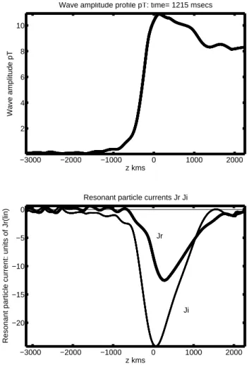
Fig. 7. Run 1. Wave amplitude at the exit from the simulation box as a function of time; note the build up over 1/2 s, and then saturation at t = 1.215 s. −3000 −2000 −1000 0 1000 2000 2 4 6 8 10 z kms Wave amplitude pT
Wave amplitude profile pT: time= 1215 msecs
−3000 −2000 −1000 0 1000 2000 −20 −15 −10 −5 0
Resonant particle currents Jr Ji
z kms
Resonant particle current: units of Jr(lin)
Jr
Ji
Fig. 8. Run 1. Snapshot at t = 1.215 s of wave amplitude, the in phase current Jr, and out of phase current JIas functions of z. Note
the characteristic structure of a dynamically stable riser generation region.
riser. The simulation uses the following data: L = 3.4;
−3000 −2500 −2000 −1500 −1000 −500 0 500 1000 1500 2000 −1000 −800 −600 −400 −200 0 200 400 600 800 z kms d/dz(Ji/|R| Hz/s
Plot of phi=Ad/dz(Ji/R) Hz/s and |R| pT
Fig. 9. Run 1. Plot of wave amplitude R = |E| (dashed line) and
8 = A d/dz{Ji/R}(solid line) as functions of z at t = 1.1 s. Note
the generally positive value of 8 ∼ +400 Hz/s.
input field magnitude Bin = 0.1 pT; saturation amplitude
Bmax=8.8 pT; linear equatorial growth rate γlin=78 dB/s;
cold plasma density N e = 800/cc; input pulse length = 1 s; f =10200 Hz. With these data the integrated linear amplifi-cation along the field line at the trigger frequency is ∼15 dB. This is only a little more than the figure of 14 dB calculated by Bell et al. (2000) from actual measurements of the par-ticle fluxes, though for this figure they make the reasonable assumption that the anisotropy extends to beyond the mea-sured maximum energy of 20 keV.
Figure 6 shows the frequency-time spectrogram derived from the wave field data stream exiting from the receiver side of the simulation box. The time t = 0 is that at which the leading edge of the triggering pulse exits from the simulation box. The spectrogram is presented as a shaded MATLAB contour plot, and shows the triggering, before the end of the initial pulse, of a strong riser with a sweep rate ∼ +2 kHz/s. Figure 7 shows the exit field amplitude as a function of time. The amplitude rises gradually to the saturation level over a period ∼0.5 s, but this is nothing like the slow exponen-tial growth reported in some Siple experiments (Helliwell, 1983). Further, there are oscillations due to the sideband instability. Figure 8 represents a snapshot at t = 1.215 s of the wave amplitude profile in the spatial box, and also shows the profiles of the resonant particle current component in phase with the wave electric field (Jr)and that in phase
with the wave magnetic field (Ji). Here z = 0 is the
equa-tor. Note that the in phase current gives (nonlinear) a wave growth proportional to −Jr, and that the out of phase
cur-rent JI changes the wave phase at a rate of AJi/|E|(Nunn,
1990, 1993). What we see here is essentially the nonlinear generation region (GR) of a triggered rising frequency VLF emission. This is a surprisingly stable dynamical structure not unlike a soliton in its behaviour. The form of the resonant particle current is readily understood as being due to phase trapping of cyclotron resonant electrons in the parabolic
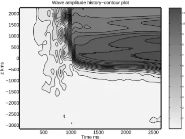
in-500 1000 1500 2000 2500 −3000 −2500 −2000 −1500 −1000 −500 0 500 1000 1500 2000 Time ms z kms
Wave amplitude history−contour plot
1 2 3 4 5 6 7 8 9 10 11
Fig. 10. Run 1. Exit wave amplitude (pT) history of the entire simulation as a contour plot in the z, t plane. Note the stable quasi-static envelope of the riser GR. Units of the grey scale are arbitrary.
500 1000 1500 2000 2500 −3000 −2500 −2000 −1500 −1000 −500 0 500 1000 1500 2000 Time ms z kms
In phase resonant particle current (Jr) history−contour plot
0 5 10 15 20 25
Fig. 11. Run 1. History of in phase current −Jr in the
simula-tion box, in units of Jr(lin); this component gives nonlinear wave
growth. The steady increase with time relates to the rising frequency of the emission, increasing resonant electron fluxes, and increasing growth rates.
homogeneity. Figure 9 shows the same snapshot and plots the quantity 8 = A d/dz(Ji/R)in Hz/s, where R = |E|. It
was shown in Nunn (1993) that 8 is the local rate of change of frequency due to the resonant particle current having a wavelength shifted from that of the in situ wave. It should be pointed out though that in a VLF emission generating region, a sizeable spatial gradient of wave number is set up, and the overall sweep rate seen by a stationary observer is due mainly to this. The graph reasonably shows a pronounced positive value in the GR of 8 ∼ +400 Hz/s.
The next three graphs (Figs. 10–12) give a history of the entire simulation. They are contour plots of wave
ampli-500 1000 1500 2000 2500 −3000 −2500 −2000 −1500 −1000 −500 0 500 1000 1500 2000 Time ms z kms
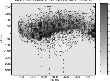
Out of phase resonant particle current (Ji) history−contour plot
0 5 10 15 20 25 30 35 40 45 50
Fig. 12. Run 1. History of out of phase current −Ji, which changes
the wave phase, in units of Jr(lin). The steady increase with time
relates to the rising frequency of the emission, increasing resonant electron fluxes, and increasing growth rates.
tude (in pT), in-phase current Jr and out of phase current Ji,
the latter in units of Jr(lin), the linear equatorial current that
would result at the triggering frequency and at the saturation amplitude. The most remarkable feature is the almost static nature and stability of the riser GR. This is a strongly non-linear case, with particles being trapped for many trapping periods. The nonlinear currents rise steadily with time, since the particle fluxes and linear growth rates increase with rising frequency. The overall current magnitudes go from ∼5 times linear to ∼25 times. This is an important result. Nonlinear growth rates are normally of the same sign as the linear one and larger by a factor of the order of the number of trapping periods for which resonant particles are trapped. Nonlinear growth rates may, therefore, be many times larger than linear ones.
The second run is a simulation of a faller. The parameters used are the same as for run 1, except that the linear equa-torial growth rate is higher, at 80 dB/s, the saturation level is set at 6 pT, giving a weaker degree of nonlinearity, and the simulation bandwidth is 22 Hz. Figure 13 shows the spectro-gram of the exit wave field data stream: a vigorous faller is triggered before the initial pulse ends. The sweep rate is very stable at −2000 Hz/s, and the emission terminates at 1.6 s due to the falling power input due to the decreasing frequency and corresponding increasing resonance velocity. Figure 14 gives a snapshot of the wave profile and 8 = A d/dz(Ji/R)
{Hz/s} at t = 1.0 s. The latter has a pronounced negative region ∼ −400 Hz/s, but becomes positive in the far tail of the GR. Note again that the sweep rate in a faller is mainly due to the establishment of a negative wave-number gradient across the GR.
It is of some interest to examine the behaviour of the distri-bution function in velocity space in the neighbourhood of the resonance velocity. Considering the |V ⊥ | “beam” with a
0.2 0.4 0.6 0.8 1 1.2 1.4 1.6 8600 8800 9000 9200 9400 9600 9800 10000 10200 Time secs Frequency Hz
Frequency/time plot of VLF emission
Fig. 13. Run 2. Omega triggered faller.
−2000 −1500 −1000 −500 0 500 1000 1500 −600 −400 −200 0 200 400 600 800 z kms d/dz(Ji/|R| Hz/s
Plot of phi=Ad/dz(Ji/R) Hz/s and |R| pT
Fig. 14. Run 2. Plot of wave profile R = |E| (dashed line) and
8(solid line) as functions of z at t = 1.0 s. Note the pronounced region where 8 is negative and the fact that the wave profile extends further upstream (towards the transmitter) in the case of a faller GR.
pitch angle of 71 degrees, Fig. 16 plots the integrated energy change dW (proportional to dF) as a function of gyrophase relative to the wave E field (ψ ) and V∗=V
z−Vresin units
of “trapping widths”. This is at the location z = +447 km on the receiver side of the equator, where inhomogeneity is negative and the phase locking (or trapping) angle lies in the quadrant 180–270 degrees, (Nunn, 1990). The “bunch” of stably trapped resonant electrons, defined by a large positive dW, manifests itself at once, and defines the physical location of the trap in ψ, V∗space. There is a popular misconception that the electrons trapped by the wave alone provide the en-ergy for wave amplification. Here trapped electrons are ac-celerated, but untrapped electrons give up more energy to the wave-field, giving net growth.
−2 −1 0 1 2 0 100 200 300 400 −0.04 −0.02 0 0.02 0.04 0.06
V||−trapping widths about Vres
Surface plot of dW; z= −42.74
Gyrophase of Vp wrt E−degs
Integrated particle energy change
Fig. 15. Run 2. Surface plot of dW, the integrated particle energy change in dimensionless units, in the V∗, ψ plane, for the |V ⊥ | beam with a pitch angle of 71 degrees; recorded at t = 1.0 s and at z = −42.7 km (on the ground TX side). The stably trapped particles in the “trap” correspond to the large positive values of dW. The gyrophase ψ is the phase of the V ⊥ vector relative to wave electric field. −2 −1 0 1 2 0 100 200 300 400 −0.02 −0.01 0 0.01 0.02 0.03
V||−trapping widths about Vres
Surface plot of dW; z= 447.2
Gyrophase of Vp wrt E−degs
Integrated particle energy change
Fig. 16. Run 2. Surface plot of dW, but at z = 447.2 km.
Figure 15 shows the same data further upstream, at z = −43 km. An overall positive contribution to dW is seen due to the start of trapping in the positive inhomogeneity, with negative peaks due to the history of trapping in the negative inhomogeneity region.
The final run (run 3) is with a much larger growth rate of 110 dB/s, strong nonlinearity being provided by a saturation amplitude of 9 pT, with an input amplitude of 0.12 pT, and a wider simulation bandwidth of 44 Hz. Trans-equatorial am-plification is now 22 dB, somewhat higher than the values considered by Bell et al. (2000). Strong power input often results in an oscillatory emission or “wandering tone” and
0.5 1 1.5 2 2.5 3 1 1.05 1.1 1.15 1.2 1.25 x 10⁴ Time secs Frequency Hz
Frequency/time plot of VLF emission
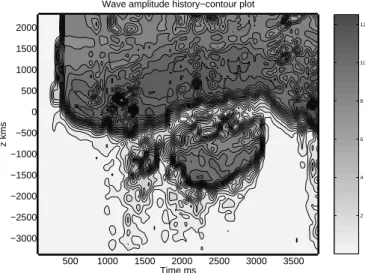
Fig. 17. Run 3. Omega triggered oscillating frequency emission. This kind of behaviour requires a high linear growth rate, here 110 dB/s. 500 1000 1500 2000 2500 3000 3500 −3000 −2500 −2000 −1500 −1000 −500 0 500 1000 1500 2000 Time ms z kms
Wave amplitude history−contour plot
2 4 6 8 10 12
Fig. 18. Run 3. Wave amplitude (pT) history of the simulation. The central region from t = 1.5 s to t = 3.0 s corresponds to a faller GR, which extends further upstream into the positive inhomogene-ity region. Note the consistent amplitude trough in the vicininhomogene-ity of the equator at z ∼ −500 km. This is a region of damping which occurs when the phase trapping angle moves between quadrants.
that is shown in the case here. Figure 17 shows the spec-trogram of the output field. Triggering takes place almost at once at t = 0.2 s, and a riser is produced with a sweep rate ∼1 kHz/s. This becomes a faller at 1.6 s and again a riser at 3.0 s. The next three graphs (Figs. 18–20) give a “history” of the event by plotting field wave field amplitude and the cur-rents Jr and Jiin the z, t plane. The generation region of the
faller (t = 1.5 to 3.0 s) extends further upstream (towards the transmitter) into the positive inhomogeneity region, where Ji
becomes positive and 8 = A d/dz(Ji/R)becomes negative
(Nunn, 1997, 1999). The latter term is responsible for
set-500 1000 1500 2000 2500 3000 3500 −3000 −2500 −2000 −1500 −1000 −500 0 500 1000 1500 2000 Time ms z kms
In phase resonant particle current (Jr) history−contour plot
−5 0 5 10 15 20
Fig. 19. Run 3. History of in phase current −Jrin units of Jr(lin).
Large positive values are evident 500 km upstream from the “am-plitude trough”.
ting up the negative wave-number gradients that cause the falling frequency. A noticeable feature of the faller GR is the consistent trough in wave amplitude just upstream from the equator. The Jr values become positive in this region,
giv-ing wave dampgiv-ing. By contrast the riser generation region is confined almost entirely downstream of the equator in the negative inhomogeneity region, where Ji is negative and 8
positive. Both riser and faller GRs are distinct and differ-ent stable dynamical structures. Transitions between the two may occur. Clearly, excess power, such as that which may occur with increasing frequency, will extend the wave profile upstream and change the GR into the faller type. Conversely, decreasing power, such as that which occurs with falling fre-quency, will either cause the wave profile to slip downstream and convert a faller GR into a riser GR, or else cause the termination of the emission. The increased oscillations in the plots are due to sideband activity permitted by the larger bandwidth of the simulation.
5 Conclusions
Bell et al. (2000) have reported useful, interesting and impor-tant observations of electron distribution functions in space at L∼3.4. For the energy range 1–20 keV “pancake” distribu-tions with very high anisotropies were observed consistently. They suggested that such new distribution functions would radically alter existing theories of triggered VLF emissions and chorus, based on the nonlinear trapping of cyclotron resonant electrons in a parabolic (B field) inhomogeneity. When the relative contributions of different pitch angles to the linear and nonlinear growth of Omega VLF pulses were investigated, however, it was found that the “pancake” dis-tribution functions did not make too much of a difference. The range of pitch angles providing the maximum power
500 1000 1500 2000 2500 3000 3500 −3000 −2500 −2000 −1500 −1000 −500 0 500 1000 1500 2000 Time ms z kms
Out of phase resonant particle current (Ji) history−contour plot
−5 0 5 10 15 20 25 30 35 40 45
Fig. 20. Run 3. History of out of phase current −JI in units of
Jr(lin). In the faller GR, positive values are encountered upstream
of the equator, which are directly instrumental in modifying wave phase such that wave frequency falls.
increased from ∼53–67 degrees to ∼67–77 degrees. For a fixed wave amplitude the degree of particle nonlinearity fell by only a small amount.
The space borne observations of distribution functions and actual energetic electron fluxes represent a priceless real data input to the theoretical problem of triggered VLF emissions. To make the most use of the data we decided to use a 1-D VHS code to simulate Omega triggered emissions with the Bell et al. (2000) “pancake” distribution function. Risers, fallers, hooks and oscillating tones were all simulated. Inter-estingly, the integrated trans-equatorial linear growth ∼15 dB used in the simulations (an indicator of particle fluxes) was only slightly larger than those calculated by Bell et al. (2000) from real data, though they did assume that the particle anisotropy extended beyond 20 keV, the limit of their mea-surements.
What are we to conclude? Certainly nonlinear trapping theory remains the only credible theory of triggered emis-sions and chorus on the table at the moment, though one must always remain receptive of new ideas and theories. Difficul-ties do remain, however; notably these are of understanding the saturation mechanism (nonlinear unducting) , the mech-anism whereby one chorus element triggers the next, and the reason why triggered emissions stay in so narrow a band when theoretically, the nonlinear wave particle interaction process is upper sideband unstable.
It is important that the scientific community does not get too carried away by these exciting new observations. It is not certain that “pancake” distribution functions are universal at L =3.4, let alone anywhere else. Satellite observations from Geotail at L = 10 showed quite low particle anisotropies, but discrete emissions were nonetheless simulated using this same VHS code (Nunn et al., 1997). Clearly, chorus and triggered/discrete emissions occur in a wide variety of
lo-cation in the near-Earth space environment, not to mention in Jupiter’s magnetosphere. The underlying plasma physi-cal mechanism is obviously the same. It would be a matter of some surprise if a “pancake” distribution observed at one location invalidated the theory.
Acknowledgements. All the authors acknowledge the financial
sup-port from NATO Linkage Grant EST.CLG 975144 and from INTAS grant 99-00502.
Topical Editor G. Chanteur thanks D. Shklyar and another ref-eree for their help in evaluating this paper.
References
Bell, T. F., Inan, U. S., Helliwell, R. A., and Scudder, J. D.: Simul-taneous triggered VLF emissions and energetic electron distri-butions observed on POLAR with PWI and HYDRA, Geophys. Res. Lett., 27(2), 165–168, 2000.
Carlson, C. R., Helliwell, R. A., and Inan, U. S.: Space time evo-lution of whistler mode wave growth in the magnetosphere, J. Geophys. Res., 95, 15 073, 1990.
Chanteur, G.: Vlasov simulations of ion acoustic double layers, in: Computer Simulation of Space Plasmas, Reidel, Dordrecht, 279, 1985.
Cheng, C. Z. and Knorr, G.: The integration of the Vlasov equation in configuration space, J. Comput. Phys., 22, 330, 1976. Denavit, J.: Numerical simulation of plasmas with periodic
smooth-ing on phase space, J. Comput. Phys., 9, 75, 1972.
Gurnett, D. A., et al.: The POLAR plasma wave instrument, The Global Geospace Mission, (Ed) Russell, C.T., Kluwer Academic Publishers, London, 597–622, 1995.
Helliwell, R. A.: A theory of discrete VLF emissions from the mag-netosphere, J. Geophys. Res., 72, 4773, 1967.
Helliwell, R. A., and Crystal, T. L.: A feedback model of cyclotron interaction between whistler mode and energetic electrons in the magnetosphere, J. Geophys. Res., 78, 7357, 1973.
Helliwell, R. A. and Katsufrakis, J. P.: VLF wave injection into the magnetosphere from the Siple station, Antarctica, J. Geophys. Res., 79, 2511, 1974.
Helliwell, R. A., Carpenter, D. L., and Miller, T. R.: Power thresh-old for growth of coherent VLF signals in the magnetosphere, J. Geophys. Res., 85, 3360, 1980.
Helliwell, R. A., Carpenter, D. L., Inan, U. S., and Katsufrakis, J. P.: Generation of band limited VLF noise using the Siple trans-mitter: a model for magnetospheric hiss, J. Geophys. Res., 91, 4381, 1986.
Helliwell, R. A.: Controlled stimulation of VLF emissions from Siple station, Antarctica, Radio Sci., 18, 801, 1983.
Helliwell, R. A. and Inan, U. S.: VLF wave growth and discrete emission triggering in the magnetosphere: a feedback model, J. Geophys. Res., 87, 3537, 1982.
Karpman, V. I., Istomin, Y. N., and Shklyar, D. R.: Nonlinear fre-quency shift and self modulation of the quasi-monochromatic whistlers in the inhomogeneous plasma (magnetosphere), Planet. Space Sci., 22(5), 859–871, 1974.
Molvig, K., Hilfer, G., Miller, R. H., and Myczkowski, J.: Self consistent theory of triggered VLF emissions, J. Geophys. Res., 93, 5665, 1988.
Nunn, D.: A nonlinear theory of sideband stability in ducted whistler mode waves, Planet. Space Sci., 34(5), 429–451, 1986.
Nunn, D.: The numerical simulation of VLF non-linear wave par-ticle interactions in collision free plasmas using the Vlasov Hy-brid Simulation technique, Computer Physics Comms., 60, 1–25, 1990.
Nunn, D.: A novel technique for the numerical simulation of hot collision free plasma; Vlasov Hybrid Simulation, J. Computa-tional Phys., 108(1), 180–196, 1993.
Nunn, D., Omura, Y., Matsumoto, H., Nagano, I., and Yagitani, S.: The numerical simulation of VLF chorus and discrete emissions observed on the Geotail satellite using a Vlasov code, J. Geo-phys. Res., 102, 27 083–27 097, 1997.
Nunn, D., Manninen, J., Turunen, T., Trakhtengerts, V., and Erokhin, N.: On the nonlinear triggering of VLF emissions by power line harmonic radiation, Ann. Geophysicae, 17, 79–94, 1999.
Omura, Y. and Matsumoto, H.: Computer simulations of basic pro-cesses of coherent whistler wave particle interactions in the mag-netosphere, J. Geophys. Res., 87, 4435, 1982.
Omura, Y., Nunn, D., Matsumoto, H., and Rycroft, M. J.: A review of observational, theoretical and numerical studies of triggered VLF emissions, J. Atmos. and Terr. Phys., 53, 351–368, 1991. Pasmanik, D. L., Nunn, D., Demekhov, A. G., Trakhtengerts, V. Y.,
and Rycroft, M. J.: Cyclotron amplification of whistler waves:
a parametric study relevant to the nature of discrete VLF emis-sions, Submitted to J. Geophys. Res., 2001.
Roux, A. and Pellat, R.: A theory of triggered VLF emissions, J. Geophys. Res., 95, 12 277, 1978.
Sa, L. A. D.: A wave-particle-wave interaction mechanism as a cause of triggered VLF emissions, J. Geophys. Res., 95, 12 277, 1990.
Scudder, J., et al.: Hydra- a 3-dimensional electron and ion hot plasma instrument for the Polar spacecraft of the GGS mission, in: The Global Geospace Mission, (Ed) Russel, C. T., Kluwer Academic Publishers, 459–495, 1995.
Smith, A. J. and Nunn, D.: Numerical simulation of VLF risers, fall-ers and hooks observed in Antarctica, J. Geophys. Res., 103(A4), 6771–6784, 1998.
Trakhtengerts, V. Y., Demekhov, A. G., Pasmanik, D. L., Titova, E. E., Kozelov, B. B., Nunn, D., and Rycroft, M. J.: Highly anisotropic distributions of energetic electrons and triggered VLF emissions, Geophys. Res. Letts., 28(13), 2577–2579, 2001. Trakhtengerts, V. Y., Rycroft, M. J., and Demekhov, A. G.: Inter-relation of noiselike and discrete ELF/VLF emissions generated by cyclotron interactions, J. Geophys. Res., 101, 13 293–13 301, 1996.