Direct Simulation and Deterministic Prediction of
Large-scale Nonlinear Ocean Wave-field
by
Guangyu Wu
B.S., University of Science and Technology of China (1994)
M.Eng., Chinese Academy of Sciences (1997)
Submitted to the Department of Ocean Engineering
in partial fulfillment of the requirements for the degree of
Doctor of Philosophy
at the
MASSACHUSETTS INSTITUTE OF TECHNOLOGY
June 2004
Massachusetts Institute of Technology 2004. All rights reserved.
A uthor ... ...
Department of Ocean Engineering
May 26, 2004
Certified by ....
...
Dick K.P. Yue
Professor of Hydrodynamics and Ocean Engineering
Thesis Supervisor
Accepted by...
...
Michael S. Triantafyllou
Professor of Ocean Engineering
Chairman, Committee for Graduate Students
MASSACHUSETTS INSITrhTE
OF TECHNOLOGY
SEP 0 1 2005
BARKER
Direct Simulation and Deterministic Prediction of
Large-scale Nonlinear Ocean Wave-field
by
Guangyu Wu
Submitted to the Department of Ocean Engineering on May 26, 2004, in partial fulfillment of the
requirements for the degree of Doctor of Philosophy
Abstract
Despite its coarse approximation of physics, the phase-averaged wave spectrum model has been the only type of tool available for ocean wave prediction in the past 60 years. With the rapid advances in sensing technology, phase-resolved nonlinear wave modeling, and high performance computing capability in recent years, the time has come to start developing a new generation tool for ocean wave prediction using di-rect phase-resolved simulations. The key issues in developing such a tool are: (i) proper specification of initial/boundary conditions of the nonlinear ocean wave-field; (ii) development of efficient algorithm for simulation of large-scale wave-field evolu-tion on high performance computing platforms; (iii) modeling of nonlinear physics in ocean wave evolution such as wave-wave, wave-current, wave-bottom and wave-wind interactions. The objective of this thesis is to address (i), (ii) and part of (iii).
For (i), a multi-level iterative wave reconstruction tool is developed to deter-ministically reconstruct a nonlinear ocean wave-field based on single or multiple wave probe records, using both analytic low-order Stokes solutions and High-Order-Spectral (HOS) nonlinear wave model. With the reconstructed wave-field as the initial con-ditions, the ocean wave-field can then be simulated and forecasted into the future deterministically with the physics-based phase-resolved wave model. A theoretical framework is developed to provide the validity of the reconstructed wave-field and the predictability of future evolution of the reconstructed wave-field for given wave conditions. The effects of moving probe, ambient current and finite water depth on the predictable region are studied respectively. To demonstrate its efficacy and useful-ness, the wave reconstruction tool is applied to reconstruct the full kinematics of steep two- and three-dimensional irregular waves using both wave-basin measurements and synthetic data. Excellent agreements between the reconstructed nonlinear wave-field and the original specified wave data are obtained. In particular, it is shown that the inclusion of high-order effects in wave reconstruction is of significance, especially for the prediction of the wave kinematics such as velocity and acceleration.
For (ii), a highly scalable HOS wave model is developed and applied to study both two- and three-dimensional ocean wave-field evolution for a realistic space and time
scale. Effective filtering tools are developed to model the wave breaking process in wave evolution. For (iii), the HOS wave model is enhanced to account for not only nonlinear wave-wave interactions, but also nonlinear wave interaction with variable ambient current. With this tool, the effects of variable ambient current on nonlinear wave-field evolution are investigated.
As a final illustration, this tool is applied in practical ship motion control. Based on the deterministically forecasted wave-field provided by this tool, an optimal path is obtained to reduce the RMS heave motion of ship in point-to-point transit.
Thesis Supervisor: Dick K.P. Yue
Title: Professor of Hydrodynamics and Ocean Engineering
Acknowledgments
Firstly, I would like to thank Professor Dick K.P. Yue, my thesis advisor, for his continuous guiding and helping me to gradually become mature and experienced both as an individual and as a scientific researcher. I am grateful for having the opportunity to work with him during the past seven years.
I owe my special thanks to Dr. Yuming Liu. Without his encouragement and tremendous help during the lows of the research, I would have never come to this point.
I want to thank Professor Nicholas M. Patrikalakis and Professor Nicholas C. Makris for serving on my thesis committee, and for the invaluable time and effort they have spent to help me in such an important stage of my life. I benefited a lot from their comments and suggestions on my thesis research.
I would also like to thank my colleagues in Vortical Flow Research Laboratory. In particular, I am indebted to Kelli L. Hendrickson and Benjamin S.H. Connell, not only for their great friendship which makes my life here more memorable, but also for their dedication to system administration of the laboratory which allows me to focus more on my research.
Finally, I dedicate this thesis to my wife, Zhoutao, for her endless support through-out all these years, and to my little son, Ryan, for the joy and inspiration he brings to me.
This research is financially supported by the Office of Naval Research and the Defense Advanced Research Projects Agency.
Contents
1 Introduction
1.1 Nonlinear wave dynamics and HOS 1.2 Data assimilation and initial conditions 1.3 Variable ambient current . . . . 1.4 Variable bottom topography . . . . 1.5 Wave dissipation due to breaking . . . . 1.6 Wave dissipation due to bottom friction. 1.7 W ind input . . . . 1.8 Thesis objective, approach, and outline .
2 Theory on deterministic predictability of ocean waves
2.1 B ackground . . . . 2.1.1 M otivation . . . . 2.1.2 Existing study in wave forecasting . . . . 2.1.3 Present study . . . . 2.2 Problem statement . . . . 2.3 Basic assumptions . . . . 2.4 Characteristics of ocean wave spectrum . . . . 2.5 Unidirectional wave predictability . . . .
2.5.1 Predictability of unidirectional wave based on single probe record 2.5.2 Prediction error of unidirectional wave outside the predictable
region . . . . 2.6 Multi-directional wave predictability . . . .
7 27 . . . . . 28 . . . . . 29 . . . . . 30 . . . . . 31 . . . . . 31 . . . . . 31 32 32 35 35 35 36 37 38 39 40 43 43 48 51
2.6.1 Predictability of directional wave based on decomposition of
single probe record . . . . 54
2.6.2 Prediction error outside the predictable region . . . . 61
2.7 Nonlinear effect in ocean wave predictability . . . . 61
2.8 Effects of probe motion, finite water depth, and ambient current . . . 65
2.8.1 Effect of probe motion . . . . 65
2.8.2 Effect of finite water depth . . . . 67
2.8.3 Effect of ambient current . . . . 68
2.9 Combined predictability of multiple probe records . . . . 72
2.9.1 Two-dimensional wave . . . . 72
2.9.2 Three-dimensional wave-field . . . . 73
2.10 Sum m ary . . . . 75
3 Multilevel nonlinear ocean wave reconstruction and forecasting 79 3.1 Background . . . . 79
3.1.1 Present study . . . . 80
3.2 High-order-spectral method . . . . 81
3.3 Multilevel nonlinear wave reconstruction and forecasting scheme . . . 82
3.3.1 Free wave components description . . . . 85
3.3.2 Definition of wave reconstruction error . . . . 86
3.3.3 Weighting function . . . . 87
3.3.4 Optimization schemes . . . . 87
3.3.5 Uniqueness of wave reconstruction . . . . 91
3.3.6 Direction resolvability and position of probes . . . . 93
3.3.7 Importance of optimizing direction of wave components . . . . 97
3.3.8 Continuous ocean wave representation . . . . 98
3.4 Computational effort estimation . . . . 100
3.5 Convergence test . . . . 102
3.6 Numerical verification of predictability theory . . . . 103
3.6.1 Two-dimensional case . . . . 103
3.6.2 Three-dimensional case . . . .
3.6.3 Importance of capturing nonlinearity in wave reconstruction .
3.6.4 Effect of probe motion . . . .
3.6.5 Importance of proper accounting for finite water depth . . . . 3.6.6 Importance of proper accounting for ambient current . . . . . 3.7 Wave reconstruction based on multiple probe records . . . .
3.8 Comparison of two-dimensional experiments with nonlinear wave re-construction . . . . 3.8.1 TAMU experiment . . . .
3.8.2 Wave elevation comparison . . . .
3.8.3 Importance of nonlinearity in wave kinematics and dynamics
reconstruction . . . .
3.8.4 Deterministic wave forecasting . . . .
3.8.5 Long-time nonlinear irregular wave reconstruction . . . .
3.9 Comparison with three-dimensional Bull's Eye wave experiments . . . 3.9.1 Experim ent . . . .
3.9.2 Reconstruction results . . . .
3.10 Sum m ary . . . .
4 Phase-resolved simulation of nonlinear wave spectrum evolution 4.1 Background . . . .
4.1.1 Present study . . . . 4.2 Generation of deterministic initial condition from spectrum . 4.2.1 Linear initial conditions . . . . 4.2.2 Initial stage of simulation . . . . 4.3 Evaluation of wave spectrum . . . . 4.3.1 Obtain wavenumber spectrum . . . . 4.3.2 Wavenumber spectrum to frequency spectrum . . . .
4.4 Wave breaking model . . . . 4.5 Two-dimensional spectrum evolution . . . .
. . . . . 147 . . . . . 148 . . . . . 149 . . . . . 150 . . . . . 152 . . . . . 154 . . . . . 154 . . . . . 155 . . . . . 158 . . . . . 159 9 107 111 111 114 114 117 126 126 127 128 135 136 140 140 140 142 147
4.6 4.7 4.8
Three-dimensional spectrum evolution . . . . Reconstruction of two-dimensional nonlinear wave spectrum . . . . .
Sum m ary . . . .
164 167 170
5 Ambient current effect on wave characteristics 171
5.1 Background ... ... .. 171
5.1.1 Collinear current . . . . 173
5.1.2 Shearing current . . . . 175
5.1.3 Other existing studies on wave-current interaction . . . . 177
5.1.4 Present study . . . . 178
5.2 Governing equations . . . . 179
5.3 First-order asymptotic solution for collinear current case . . . . 182
5.4 Change of wave characteristics with collinear current . . . . 184
5.4.1 Current profile . . . . 185
5.4.2 Numerical wave damping . . . . 185
5.4.3 Following current . . . . 186
5.4.4 Opposing current . . . . 190
5.4.5 Wave reflection/blocking in opposing current . . . . 193
5.5 Ocean wave evolution in variable current . . . . 201
5.5.1 Ocean waves moving on collinear variable current . . . . 201
5.6 Ocean waves propagating on horizontal shearing current . . . . 203
5.7 Sum m ary . . . . 203
6 Effect of measurement noise on wave reconstruction 209 6.1 Background . . . . 209
6.1.1 Present study . . . . 210
6.2 Monte-Carlo simulation . . . . 210
6.3 Sum m ary . . . . 212
7 Practical applications
7.1 Simulation of large-scale long-time ocean wave-field evolution . . . .
217 217
7.1.1 Computational effort requirement . . . . 217
7.1.2 Case demonstration . . . . 219
7.2 Application in ship motion control . . . . 221
8 Conclusions and suggestions for future work 223 8.1 Conclusions . . . . 223
8.1.1 Ocean wave prediction . . . . 224
8.1.2 Ambient current effect . . . . 224
8.1.3 Wave spectrum evolution . . . . 224
8.2 Future work . . . . 225
8.2.1 Wave reconstruction in combined predictable region using mul-tiple probe records . . . . 225
8.2.2 Reconstructing Waves from hybrid sensing data . . . . 225
A Linear, second-order Stokes and high-order HOS representations of irregular wave-field 227 A.1 Linear irregular wave model . . . . 227
A.2 Second-order irregular wave model . . . . 229
A.3 High-Order-Spectral (HOS) wave model . . . . 233
B Nonlinear dispersion relation 239 C Polynomial noise 241 C.1 Statistic HO S . . . . 242
C.2 Num erical case . . . . 246
C.3 Computational effort limitation . . . . 247
List of Figures
2-1 Sketch of the wave reconstruction problem in a directional ocean wave-field . . . . 39 2-2 P-M spectrum and JONSWAP spectrum. . . . . 41 2-3 Cosine-square angular spreading function. . . . . 43 2-4 Predictable region of a two-dimensional ocean wave-field, with the
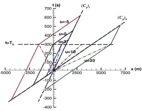
slowest and fastest group velocities Cg1 and C h, based on the mea-surement of a probe at xz0 in the time interval 0 < t < T. . . . . . 46 2-5 Error in predicting the wave property at a point outside the predictable
region based on measurement at x = 0 with t E [0, To]. : wave
dis-turbance measured by the probe; - - -: wave disturbance not measured by the probe. ... ... 49 2-6 Error contour in predicting the wave property at an arbitrary point
in wave-field based on measurement at x = 0. (a) JONSWAP spec-trum; (b) P-M spectrum. The region enclosed by the white line is the predictable region. . . . . 50 2-7 Cross-cut plots of Figure 2-6: (a) x=1000m; (b) t=360s. :
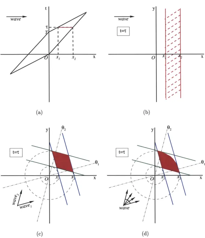
JON-SWAP spectrum; - - -: P-M spectrum. . . . . 52 2-8 Three-dimensional wave prediction extended from two-dimensional
the-ory. (a) Two-dimensional predictable region at t = T: [XI, X2]; (b)
predictable region of unidirectional wave in two-dimensional horizon-tal space; (c) predictable region of waves with two directional compo-nents; (d) predictable region of waves consists of components moving with directions within [01, 021. . . . . 53
2-9 Two kinds of predictable regions for t T < 0. (a) Predictable region
is enclosed by (abc); (b) predictable region is enclosed by (abcde). . . 55
2-10 Predictable region for 0
<t
= T . . . . 572-11 Two kinds of predictable regions for t = T > T. (a) Predictable region is enclosed by (abcde); (b) predictable region is enclosed by (abc). . . 58
2-12 Directional wave predictable region based on measurement at a fixed p oint. . . . . 60
2-13 Error in predicting the wave property at an arbitrary point in a three-dimensional wave-field based on measurements at x = 0. (a) t = 0; (b) t = T. The region enclosed by white lines is the predictable region. . 62 2-14 The nonlinear effect on predictable region. (a)Group velocity changes due to nonlinear dispersion relation; (b) predictable region changes due to nonlinear dispersion relation (T = 300s). , linear; -, (ka), = 0.1; , (ka), = 0.2; , (ka)e = 0.3; - - -, wave spectrum. 64 2-15 Effect of probe moving velocity on the predictable region. Dashed lines represent the wave record measured by the probe. . . . . 67
2-16 Effect of water depth on the group velocity . . . . 69
2-17 Effect of water depth on the predictable region. . . . . 69
2-18 Effect of current on the group velocity. . . . . 71
2-19 Effect of current on the predictable region. . . . . 71
2-20 Predictable region of an irregular wave-field, with the slowest and fastest group velocities CL and CH, based on the measurements of two probes at x=0 and x=CLT in the time interval 0 < t < T. . . . . 74
2-21 Comparison of combined predictable region of multiple probes with individual predictable regions at four time moments. (a) t = -105(s); (b) t = 0(s); (c) t = 300(s); (d)t = 390(s). - - -(green, black and blue): predictable region based on single probe; (red): combined predictable region from all three probes. . . . . 76
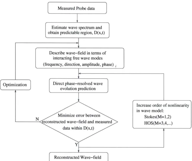
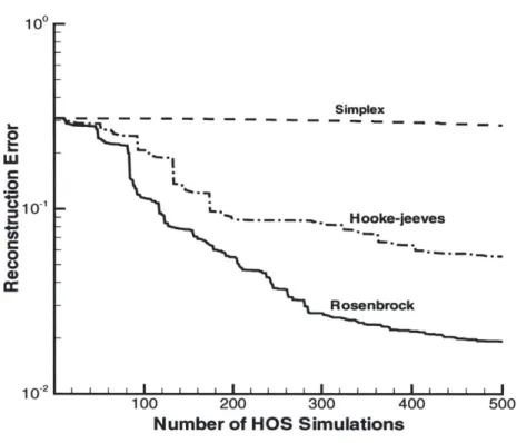
3-1 Flow chart of multilevel iterative optimization procedure for nonlinear wave reconstruction from probe measurements. . . . . 84 3-2 Comparison of different optimization schemes for HOS wave
recon-struction. : Rosenbrock method; - - -: Hooke-jeeves method; - - : Simplex method. . . . . 89
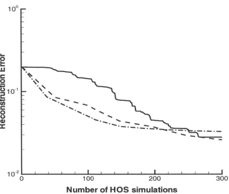
3-3 Comparison of different optimization schemes for HOS wave
recon-struction. : Rosenbrock method; - - -: Conjugate-gradient method;
- - : Quasi-Newton method. . . . . 90 3-4 Effect of the probe array geometry on wave reconstruction. Plotted
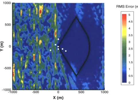
are the absolute error contour between the original wave-field and the reconstructed wave-field at time t = 0. (a) Regular array; (b) irregular array. The dark lines are the theoretically predictable region. The white circles are the positions of the probe array. . . . . 96 3-5 Effect of the probe array geometry on wave reconstruction. Plotted
is the absolute error contour between the original wave-field and the reconstructed wave-field at time t = 0. The dark lines are the
theo-retically predictable region. The white circles are the positions of the probe array. . . . . 98 3-6 Importance of including directions as optimization variables in wave
reconstruction. Plotted is the error contour at t = 0. The region en-closed by black lines is the theoretical predictable region. (a) Without direction optimization; (b) with direction optimization. . . . . 99 3-7 Reconstruction error when using different representations. (a) Discrete
representation; (b) continuous representation using Chebyshev series. 101 3-8 Convergence test. (a) Comparison of reconstructed wave record with
probe wave record: -- , probe wave record; - - -, wave reconstruction
with K 3, NW=512; -- . , wave reconstruction with K= 2, NW =
256; - - -, wave reconstruction with K_ 1, NW = 64; (b) the error between reconstructed wave record and probe record as a function of r,. 103
3-9 Verification of two-dimensional predictability theory using Monte-Carlo simulation (N, = 1000). The region enclosed by the solid line is the theoretically predictable domain. . . . . 105 3-10 Convergence test of Monte-Carlo simulations. . . . . 106 3-11 Directional wave-field reconstruction and forecasting: comparison of
reconstructed wave-field and original wave-field at fixed time point. Left: original wave-field; right: reconstructed wave-field. (a) t=0 (s); (b) t=300 (s); (c) t=360 (s). . . . . 108 3-12 Comparison of wave elevation from original wave-field and reconstructed
wave-field at cross sections at t=0. , original wave-field; - - -,
re-constructed wave-field. (a) Cross-section along the x direction at y=-1500m; (b) cross-section along the y direction at x=0. . . . . 109
3-13 Time history of elevation. original wave records; - - - - predicted
wave records. (a) x=0, y=0; (b) x=0, y=2000m. . . . . 110 3-14 Reconstruction of a nonlinear wave-field using different wave models.
Shown are the error contour between the reconstructed wave-field and the original wave-field. Region enclosed by black lines is the theoreti-cally predictable region. (a) Linear wave model; (b) second-order wave
model; (c) HOS wave model. . . . . 112 3-15 Reconstruction error when the probe is moving. - - -: moving probe
measured record; - - -: theoretically predictable region with fixed probe;
: theoretically predictable region with moving probe. . . . . 113
3-16 Reconstruction error for a wave-field with finite water depth h = 50m. Shaded area is the theoretically predictable region. (a) Correctly taking
into account the finite water depth; (b) using deep water relation. . . 115 3-17 Reconstruction error for a wave-field with current U = 0.2m/s. Shaded
area is the theoretically predictable region. (a) Correctly taking into account of the current; (b) using solution for U = 0. . . . . 116
3-18 Error contour for two-dimensional wave reconstruction based on two probe records. The reconstructed wave-field uses the same represen-tation as the one for reconstruction based on single record.
probe records; - - -: individual predictable region based on each single
probe record; -- : combined predictable region based on two probe records. ... ... 118 3-19 RMS wave reconstruction error as a function of base period. Two probe
records with t E [0, 300(s)]. . . . . 120 3-20 Successful wave reconstruction based on two probe records. Plotted is
the error contour between the reconstructed wave-field and the original
wave-field. --- : predictable region based on single probe record;
combined predictable region based on two probe records. . . . . 121 3-21 Successful wave reconstruction based on three probe records. Plotted is
the error contour between the reconstructed wave-field and the original wave-field. - - -probe records; : combined predictable region based on three probe records. ... ... 122 3-22 RMS wave reconstruction error as a function of base period.
single record (x = 0, t E [0, 300(s)]); - - -: two records (X1 = 0, x2 = 1000m, tI, t2 E [0, 300(s)]); - - -: three records (x1 = 0, x2 1000m,
X3= -100Gm, tI, t2 C [0, 300(s)], t3 E [100(s), 400(s)]). . . . . 123
3-23 Combined predictable region based on two probe records and con-structed single record for calculation of T. : combined predictable
region based on two records (x1 = 0, x2 = 1000m, tI, t2 E [0, 300(s)]); -- -: predictable region based on imaginary record (x = 0, t [tA, tB]) 124
3-24 Combined predictable region based on three probe records and con-structed single record for calculation of Tb. combined predictable
region based on three records (x1 = 0, x2 = 1000m, x3 = -1000m, tli, t2 E [0, 300(s)], t3 E [100(s), 400(s)]); - - -: predictable region based
on imaginary record (x = 0, t E [tA, tB]). . . . . 125 3-25 Experimental set-up . . . 127
3-26 Comparison of computed versus experimental free-surface elevation at the probe point as a function of time for irregular wave-fields (a) (ka)e=0.1; (b) (ka),=0.23. Plotted are: , the experimental record;
-- -, nonlinear reconstruction using HOS simulations (with NW=2048
spectral modes and order M=3); - - -, second-order reconstruction;
and - - -, linear reconstruction. . . . . 129 3-27 Comparison of computed versus experimental horizontal velocity at
the probe point as a function of vertical coordinate: A, experimental
measurement; - -- , HOS simulation with N7=2048 spectral modes and
M=3 order; - -, second-order prediction; - - -, linear prediction.
(a) (ka)e=0.1; (b) (ka),=0.23. The left part is the normal error. The right part is the velocity value at a given time point: (a) t = 114.725(s);
(b) t = 120.075(s). . . . . 131 3-28 Comparison of computed horizontal acceleration at the probe point and
a fixed time as a function of vertical coordinate: , HOS simulation
with NW=2048 spectral modes and M = 3 order; - - -, second-order prediction; - - -, linear prediction. . . . . 132 3-29 Comparison of computed Morison's inertia force on an imaginary
verti-cal cylinder as a function of time: , HOS simulation with NW=2048
spectral modes and M = 3 order; - -, second-order prediction; - - -,
linear prediction. . . . . 134 3-30 Comparison of harmonics of Morison's inertia force on an imaginary
vertical cylinder as a function of time: , HOS simulation with
NH = 2048 spectral modes and M = 3 order; - - -, second-order
prediction; - - -, linear prediction. . . . . 135 3-31 Nonlinear wave forecasting compared with experiment. (ka)e = 0.23.
(a) The wave elevation at x = 8m; (b) the wave elevation at x = 9m;
: experimental measurements; - - -: wave reconstruction and
fore-casting; - - -: indicating the theoretically predictable region. Wave
forecasting corresponds to t > T. . . . . 137 18
3-32 Comparison of computed versus experimentally measured free-surface elevation at a given point of a two-dimensional wave-field. (a) Eleva-tion as a funcEleva-tion of time; (b) Fourier Transform results, amplitude, and phase angle of elevation as a function of frequency. -- ,
experi-ments of Stansberg et al. (1995); - - -, HOS simulation with N-=16384 spectral modes and M=3 order. . . . . 138 3-33 Comparison of computed versus experimentally measured wave force
on a truncated cylinder. (a) Force as a function of time; (b) Fourier Transform results, amplitude, and phase angle of force as a function of
frequency. , experiments of Stansberg et al. (1995); - -, HOS
sim-ulation with NH=16384 spectral modes and M=3 order; - - -, second-order prediction; - - -, linear prediction. . . . . 139 3-34 Experimental setup of OTRC wave basin and wave probe positions. . 141
3-35 Comparisons of the reconstructed three-dimensional Bull's Eye wave-field to the wave-basin measurements (Liagre 1999): (a) free-surface snapshots of the wave-field from the experiment; and (b) the HOS simulation with NW=256 x 256 modes and M=3 order. . . . . 143 3-36 Comparisons of the reconstructed time history of the wave elevation to
the wave-basin measurements: (a) at probe points used in optimiza-tion, and (b) at probe points not used in optimization. From
measure-ments ( ), from HOS simulation with NW=256 x 256 modes and M = 3 order (- -) . . . . 144
4-1 The initial wavenumber spectrum for spectrum evolution simulation. (a) Two-dimensional case; (b) three-dimensional case. . . . 153
4-2 Estimation of S(wm, 0) from S(wij, Oij). . . . . 156 4-3 Comparison of the frequency spectrum obtained from the uniformly
discretized wavenumber spectrum with the original frequency spec-trum. -- : original; -- -: obtained from wavenumber spectrum. . . . 157
4-4 Comparison of numerical simulation of wave breaking due to side-band instability with experiment. A/A: amplitude of master mode in experiment/simulation; o/.: amplitude of lower sideband mode in experiment/simulation; EI/M: amplitude of higher sideband mode in experiment/simulation. . . . . 159 4-5 Energy spectrum evolution for a two-dimensional wave-field generated
from JONSWAP spectrum with -y = 3.3, a = 0.01 and wo = 1.885. (a) Wavenumber spectrum; (b) frequency spectrum. . . . . 161 4-6 Energy change in two-dimensional wave-field evolution. Significant
wave height change is also shown. . . . . 162
4-7 Energy spectrum in (k,w) space. (a) t = 0; (b) t = 500T. - - -: curves
for (w/n)2 = gk/n, n = 1, 2,3. . . . . 163 4-8 Wavenumber spectrum evolution for three-dimensional wave-field. (a)
t = 0; (b) t = 250Tp. The contour value is normalized by the peak
value of the wavenumber spectrum at t = 0. . . . . 165 4-9 Energy change in three-dimensional wave evolution. Significant wave
height change is also shown. . . . . 166 4-10 Nonlinear wave spectrum reconstruction. Black line: objective
spec-trum; green line: quasi-equilibrium spectrum using given spectrum as initial spectrum; red line: Optimized quasi-equilibrium spectrum. . . 169
5-1 The linear theory of current effect on wave characteristics. (a) Change of phase speed with collinear current; (b) change of wave number, amplitude, and steepness with collinear wave. . . . . 174 5-2 The linear theory of wave reflection in opposing current. Change of
wavenumber, amplitude, and steepness before and after reflection. . . 175 5-3 The linear theory of horizontal shearing current effect on wave
charac-teristics. (a) Change of wave direction with shearing current for differ-ent inciddiffer-ent angle; (b) change of wavenumber, amplitude and steepness with shearing current (Oo = 30 degree) . . . . 176
5-4 Computational domain setup for wave-current interaction. . . . . 185 5-5 Free-surface profile after the wave-current interaction reaches steady
state. The current profile is also shown as a reference. . . . . 187 5-6 Detailed free-surface profile after the wave-current interaction reaches
steady state. The current profile is also shown as a reference. . . . . . 188 5-7 The change of wave amplitude, wavenumber, and steepness with
cur-rent speed. The incident wave steepness is 0.001. : linear theory; *: numerical simulation. . . . . 189 5-8 The change of wave amplitude, wavenumber and steepness with current
speed. The incident wave steepness is 0.2. : linear theory; ., 0, A: amplitude, wavenumber and steepness from numerical simulation. 190 5-9 Detailed free-surface profile in an opposing current after the
wave-current interaction reaches steady state. The wave-current profile is also shown as a reference. . . . . 191 5-10 The change of wave amplitude, wavenumber, and steepness with
cur-rent speed in an opposing curcur-rent. The incident wave steepness is
0.001. : linear theory; *: numerical simulation. . . . . 192 5-11 The change of wave amplitude, wavenumber, and steepness with
cur-rent speed in an opposing curcur-rent. The incident wave steepness is 0.05.
: linear theory; o, M, A: amplitude, wavenumber, and steepness
from numerical simulation. . . . . 194
5-12 Current profile setup for wave-blocking study. Wave propagates from
left to right and current moves from right to left. x = 0 is the stopping
p oint. . . . . 197 5-13 Detailed free-surface profile when the wave is reflected by strong
oppos-ing current. (ka)' =0.001. -- : free surface elevation; - - -: current
profile. x = 0 corresponds to the stopping point from the linear theory. 198 5-14 Characteristics of incident wave and reflected wave as a function of
current velocity. (ka)'=0.001. ---- : linear theory; 0, A, o: numerical
results of amplitude, wavenumber, and wave steepness. . . . . 199
5-15 Detailed free-surface profile when the wave is reflected by strong
oppos-ing current. (ka)'=0.015. : free surface elevation; - - -: current
profile. x = 0 corresponds to the stopping point from linear theory. 200 5-16 Amplitude spectrum at x = 0 as a function of frequency for different
incident wave steepnesses. Both the amplitude and the frequency are normalized by parameters of the incident wave. From top to bottom: the incident wave steepnesses are: 0.001, 0.005, 0.01, 0.015; the local wave steepnesses at x = 0 are: 0.008, 0.04, 0.1, 0.2. . . . . 202 5-17 Surface plot of an irregular wave propagating on a collinear current.
(a) current speed profile; (b) no current case; (c) following current case: the maximum speed is 3.33m/s; (d) opposing current case: the maximum speed is 0.667m/s . . . . 204 5-18 Frequency spectra change due to a collinear current. : no current;
-- -: following current with U=3.33m/s; - - -: opposing current with U=-0.667m /s. . . . . 205 5-19 Horizontal shearing current profile. . . . 206 5-20 Surface elevation contour of a directional wave propagating through a
horizontal shearing current. (a) There is no current; (b) There is a strong horizontal shearing current . . . . 207
6-1 Original wave record and the corresponding measured record with
noise. "A": original wave record; "+": measured record with noise.
SN R = 14(dB). . . . . 212 6-2 Normalized error contour when probe measurements have noise. (a) no
noise; (b) o-/(Hs/2) = 0.025; (c) -/(H,/2) = 0.125; (d) u/(H,/2) = 0.25;213 6-3 Error increase due to noise in probe measurement for different wave
steepnesses. ... ... 214
7-1 Instantaneous surface plot of a large-scale ocean wave-field (30km x 30km ). . . . 219
7-2 Instantaneous surface plot of part of the ocean wave-field shown in Figure 7-1. Shown domain size is 2km x 2km. . . . . 220 7-3 Comparison of heave motion during ship transition for different paths.
( Courtesy of Franz S. Hover and Kenneth M. Weems.) . . . . 221
8-1 Predictable region of a two-dimensional ocean wave-field, with the slowest and fastest group velocities C91 and Cgh, based on the instan-taneous surface profile at t = 0 and x E [0, L]. . . . . 226
B-1 Definition of the angles ?mn, 6mn and 9
mn associated with wavenumber
vectors km and k.. ... ... 240
C-1 Different modes of polynomial noise as a function of x at different time. (a) t=0; (b) t=16T; (c) t=32T; (d)t=48T. -- : ?7o; : 1;
.2; - 3; . . . . 248 C-2 Amplitude of different modes of polynomial noise as a function of
wavenumber at different time. (a) t=0; (b) t=16T; (c) t=32; (d)t=48T.
- :
; : 1; _ : 12; :13; ...249
List of Tables
2.1 P-M spectrum energy distribution. . . . . 2.2 JONSWAP spectrum energy distribution .. . . . .
41 42 2.3 Maximum and minimum group velocity in nonlinear ocean waves. . . 65
3.1 Reconstruction error for wave-fields with different wave steepness. . . 106
7.1 Estimation of computational effort requirement for direct simulation of nonlinear ocean wave-field evolution . . . . 218
C.1 Number of coupled equation groups in polynomial noise representation. 247
Chapter 1
Introduction
Ocean wave-field evolution involves many complicated physical processes, including wind input via air-sea interactions, nonlinear energy transfer through wave-wave inter-actions, wave dissipation caused by surface breaking and bottom friction, and charac-teristic variations under the effect of environmental current and bottom bathymetry. It is a very challenging task to accurately predict the evolution of an ocean wave-field because details of many of these dynamic processes are still not well understood or properly modeled.
In fact, statistics-based spectral wave models such as WAM and its variations, SWAN and WAVEWATCH, are the only practical wave prediction tools available. These so-called third-generation wave models were developed based on the phase-averaged energy balance equation with all physical processes modeled as source terms. The energy balance equation can be written as:
aE
S+c .,7E=
Szn + SnI + S (.1
at
Here E is the energy density, cg the group velocity, Si, the energy input from wind,
SnI the energy transfer from nonlinear wave-wave interaction, and SdS the energy
dissipation.
Despite the progress and success of spectral wave models in the past thirty years, the inherent homogeneous and stationary assumptions, the linear transportation
equation, and the approximate source formulations have limited their further devel-opment. Dingemans (1998) gave a comprehensive review of the problems in spectral wave models and pointed out that a reconsideration is required for the basic formu-lations.
Recently, with the rapid development of computing technologies, phase-resolved direct simulations are becoming feasible alternatives to spectral wave models. Over the past fifteen years, a powerful and efficient high-order spectral method (HOS) for direct simulation of nonlinear wave dynamics has been developed and applied to the study of nonlinear wave-wave, wave-body, wave-current, and wave-bottom interactions. The efficacy of the HOS method (with exponential convergence and linear computational effort proportional to both nonlinear order M and number of modes N) enables the simulations with M ~ 0(10) and N 0 0(106-7) on today's
powerful parallel computing platforms.
Employing the fast algorithms for phase-resolved simulations of nonlinear wave dynamics, this thesis aims to develop a new-generation wave prediction model for direct simulations of large-scale nonlinear ocean wave-field evolution. In this model, for the first time, all the physical processes will be modeled, evaluated, and calibrated in a direct physics-based context. In the following sections, several key scientific processes and issues will be discussed for developing such a powerful tool, and the problems addressed by this thesis will also be identified.
1.1
Nonlinear wave dynamics and HOS
In the context of potential flow, the HOS method is capable of accounting for nonlinear wave interactions up to an arbitrary order M in the wave steepness. This enables us to effectively model the nonlinear wave-wave interactions in a broadband spectrum including: (i) energy transfer due to resonant wave-wave interactions (with quartet resonance occurring at the third order in the wave steepness and quintet at the fourth order); (ii) energy transfer due to side-band (Benjamin-Feir) instability; (iii) change of the wave kinematics due to non-resonant wave interactions; and (iv) energy cascading
to short waves due to non-resonant wave interactions.
Over the past fifteen years, the HOS method has been applied to study mech-anisms of nonlinear wave-wave interactions (Dommermuth & Yue 1987b) including the presence of atmospheric forcing (Dommermuth & Yue 1988), long-short wave in-teractions (Zhang, Hong & Yue 1993), finite depth and depth variations (Liu & Yue 1998), and submerged or floating bodies (Liu, Dommermuth & Yue 1992; Zhu 2000). To develop a new-generation wave model, we seek to extend the capabilities of the HOS method to study large-scale nonlinear ocean wave-field evolution.
1.2
Data assimilation and initial conditions
It is obvious that the above nonlinear wave dynamics can only be solved when the ini-tial conditions are available. For mechanisms study, the iniini-tial conditions are usually given as a regular wave with certain wave steepness, which can be obtained from a fully nonlinear Stokes wave solution (Schwartz, 1974), while for ocean wave-field sim-ulation, the initial wave-field is irregular and unknown. This requires an efficient data assimilation tool to generate initial conditions from observations and measurements on the ocean wave-field.
Data assimilation techniques have been used in spectral wave modeling as well. However, the initial conditions are not important because the memory of the initial conditions will vanish soon after the model starts up. The major motivation for wave data assimilation in spectral wave modeling is to improve the wind-field analysis instead of the wave-field analysis.
For the deterministic phase-resolved simulation of nonlinear wave dynamics, the accuracy of the initial conditions is critical. For short-term ocean wave-field pre-diction, deterministic free-surface elevation and wave kinematics can be accurately predicted when given accurate initial conditions. For long-term ocean wave-field pre-diction, the initial conditions have a strong effect on how the energy will transfer due to wave-wave interactions.
The major purpose of this thesis is to develop an effective data assimilation tech-29
nique that can reconstruct the two-/three-dimensional ocean wave-field from the free-surface elevation measurements of single/multiple probes. With the reconstructed wave-field as the initial conditions, we apply HOS simulations to predict the future evolution of the ocean wave-field. Chapters 2 and 3 discuss the major achievements of our research on this problem.
Hereafter, we refer to the data assimilation process of reconstructing the wave-field from measurements as wave reconstruction.
1.3
Variable ambient current
The current effect on the ocean wave-field prediction has two aspects: (1) for the wave reconstruction, correct interpretation of the measured data depends on properly accounting for the environmental current. Ignoring the existence of current can result in incorrect initial conditions; (2) for the wave simulation, the presence of a variable current can result in wave characteristics change, wave refraction, and wave reflection, which can lead to the generation of very large waves.
As a first-order physics-based model of variable current, we take into account the effect of the current on the waves while ignoring the reverse effect of the waves on the current. We also assume the total flow field is still irrotational and the current field is prescribed. To include the current effect into the direct simulation of the wave-field, we decompose the total velocity field, V, into two parts:
V(x, z, t) = U(x, z, t) + 7b (x, z, t) (1.2) Here U is the prescribed current velocity field. The boundary conditions of the nonlinear wave dynamics will be modified accordingly. Chapter 5 of this thesis dis-cusses our research on the current effects on wave characteristics for both two- and three-dimensional wave-fields. The wave reflection phenomenon is studied in partic-ular detail.
1.4
Variable bottom topography
For practical near-shore applications, finite water depth and rapidly varying bottom topography play an important role and their effects need to be considered in the prediction of nonlinear wave-field evolution. The effect of variable bottoms can be represented directly through phase-resolved simulations (Liu & Yue 1998). Signifi-cantly, non-slowly varying bottom topography is included in a straightforward way.
1.5
Wave dissipation due to breaking
With proper filtering, the phase-resolved HOS simulations are able to continue be-yond wave breaking and still obtain reasonable predictions of the post-breaking wave-field. When spilling wave breaking is present, the use of a simple low-pass filter in HOS simulation is effective in accounting for the physical energy dissipation. This has been demonstrated in the case of two-dimensional wave train evolution where HOS predictions are excellent compared to experiments well beyond the point of intense two-dimensional breaking, crescent-shaped three-dimensional breaking, and two-dimensional spilling breaking in the experiments (Dommermuth & Yue 1987a).
When plunging wave breaking is present, the use of a low-pass filter is inadequate as the energy loss in wave breaking spreads into the entire wave spectrum. In this case, a sophisticated filtering technique employing local smoothing in the physical space needs to be applied.
In this thesis, the low-pass filter and the physical-space local smoothing technique are combined to account for both types of breaking.
1.6
Wave dissipation due to bottom friction
Among different types of bottom dissipations, we consider only bottom friction be-cause it is the dominant bottom dissipation process over the continental shelves. For other special bottom conditions such as mud or permeable bed, other processes should be considered.
In general, the thickness of the turbulent bottom boundary layer is very small and the friction can be neglected for deep water waves. In the case of finite water depth, the wave motion extends down to the bottom and the bottom friction effect needs to be taken into account, especially when the bottom is rough.
To model the bottom dissipation process the direction simulation, an equivalent space-time varying viscosity can be applied to the surface waves based on the viscous dissipation in the bottom boundary layer (Ursell, 1952). This dissipation can in turn be represented as damping terms in the wave evolution boundary conditions. With this approach, the bottom dissipation is accounted for as a function of local wave characteristics and the distribution of bottom dissipation over the whole wave spectrum is obtained automatically.
1.7
Wind input
Perhaps the least known part of an ocean wave-field evolution process is the generation of waves by wind. Effective modeling of wind input due to wave-wind interactions is an extremely challenging task due to the lack of understanding of the complex dynamic processes involved. One approach is to model wind pumping as a variable pressure distribution over the free surface (Al-Zanaidi & Hui 1984) with the wind pressure specified in terms of both wave steepness and wind speed (Phillips 1963). This ignores in some sense the highly stochastic nature of the wind field (Sobey 1986) but is expected to provide realistic large-scale prediction.
1.8
Thesis objective, approach, and outline
The objective of this work is to develop a deterministic wave reconstruction and forecasting tool for a nonlinear ocean wave-field, which includes:
e reconstruction of a nonlinear ocean wave-field from single/multiple probe mea-surements of wave elevation.
" forecasting of nonlinear ocean wave-field evolution using a high-order nonlinear wave model
" demonstration of the application of the wave reconstruction and forecasting tool for large-scale wave-field evolution and practical ocean operation
To achieve this objective, this thesis
" reconstructs and forecasts a nonlinear wave-field using a multi-level optimization scheme, which can account for the arbitrary order of nonlinearity. It is scalable for high-performance computing and can be extended to hybrid-sensed wave data.
" extends HOS for simulation of large-scale ocean wave-field evolution with vari-able ambient current. It is based on the Zakhrov equation and mode-coupling, and can account for arbitrary high-order nonlinearity. The convergence is ex-ponential and the computational effort is linearly proportional to the number of wave modes and order of nonlinearity.
" implements HOS nonlinear wave models on high-performance computing plat-forms for large-scale simulations and practical applications. The computational domain size can be up to ~ O(102 3km2) and the evolution time can be up to
~ O(103-4sec.).
This thesis is organized as following: Chapter 1 introduces the problem of direct simulation wave modeling and identifies the key issues to model ocean wave dynam-ics; Chapter 2 introduces the predictability theory on deterministic reconstruction of irregular waves for both two- and three-dimensional cases; the effect of probe motion, ambient current and water depth on the predictable region are discussed; Chapter 3 introduces the multi-level nonlinear wave reconstruction scheme. The comparison between the numerical results and the experiments shows the importance of captur-ing nonlinearity in wave kinematics and dynamics reconstruction; Chapter 4 studies the wave spectrum evolution using large-scale direct simulation; Chapter 5 studies the variable ambient current effect on wave propagation; Chapter 6 studies the noise
effect on the wave simulation and reconstruction; Chapter 7 demonstrates practical applications of the deterministic wave forecasting tool. Chapter 8 discusses possible improvements in the future;
Chapter 2
Theory on deterministic
predictability of ocean waves
2.1
Background
2.1.1
Motivation
In ocean engineering applications, one of the key issues is to understand the ocean wave effect on offshore structures or vessels. To study this effect, the information of the wave-field around the structures or the vessels has to be available. However, to accurately measure the wave-field as a function of both position and time will require a very large number of probes. Therefore, in practice, people usually measure the wave-field using only a few probes and try to reconstruct the whole wave-field based on the time records from these probes. With the reconstructed wave-field, offshore structure and ship models can be evaluated for the purpose of design or performance improvement.
Wave forecasting is another key factor that can significantly affect the safety of offshore operation. Even though we know the behavior of the structures or ships under certain wave conditions and have incorporated many safety features into the design, we still do not want to run into severe wave conditions. Therefore, if we can forecast the future wave-field, we will be able to avoid severe wave conditions with an
effective control system or take certain measures in advance to protect the structure or ships. This can make the offshore operation much safer and reduce loss in human life and property damage.
2.1.2
Existing study in wave forecasting
Unfortunately, while a lot of results are obtained for regular water waves, the research on irregular ocean waves is very limited due to the complexity of the randomness. It was not until the World War II that people started to study the forecasting of ocean waves. To help the Allies in their beach-landing operation, Sverdrup and Munk developed a theory for ocean wave forecasting by introducing the concept of significant wave height and relating it to the wave amplitude in regular wave theory. Their theory was later published in U.S. Navy Hydrographic Office Publication Number 601, 1947. In 1955, Pierson introduced the stochastic process into the wave dynamics and started to use the concept of wave spectrum to describe the ocean wave-field. With the wave spectrum, all other statistical properties of the wave-field can be easily obtained. This started a new era of ocean wave modeling and forecasting. Much work has been done since that time to improve the wave spectrum model. One method that is still used worldwide by meteorologists is WAM, which was firstly developed by The WAMDI Group in 1988. Despite the success of the spectrum wave model in the prediction of wave spectrum evolution in very large spacial and/or temporal scales, they cannot obtain information on deterministic details of a wave-field, which are of critical importance for accurate modeling of complex ocean dynamic processes (such as wave breaking, wave-wind interactions, etc.) and development of wave-dodging technologies in naval operations and offshore explorations. And in the past fifteen years, almost no significant progress has been made in wave spectrum modeling, which is believed to be mainly due to the limitation of this approach.
Compared to the difficult statistical wave forecasting of ocean waves, deterministic wave forecasting seems almost impossible and the research even less abundant. The one attempt we find is by Morris et al. in 1998, in which they suggested that it is possible to forecast linear irregular wave-field deterministically for a short-term and
that the phase speed might be used to decide the predictable region. It was the first time that one realized that there is a predictable region for deterministic wave forecasting, although it will be shown in this thesis that it is the group velocity instead of the phase speed that plays the critical role in deciding the predictable region.
2.1.3
Present study
With the recent fast development of high-performance computing technology and numerical modeling of nonlinear waves, deterministic phase-resolved simulation is evolving to become an important alternative to phase-averaged statistic models for ocean wave predictions.
With deterministic wave reconstruction, one is capable of obtaining (i) the neces-sary initial conditions for deterministic simulations of nonlinear wave dynamics (and interactions with objects); (ii) the necessary kinematics for the estimation of hydro-dynamic loads on offshore structures; (iii) necessary information for phase-resolved forecasting of ocean wave evolutions; and (iv) a base for calibration/validation of experimental measurements.
Because only limited information about the original ocean waves is measured and available in wave reconstruction, the reconstructed wave-field is by no means the same as the original one. Therefore, it is important to know where and when the recon-structed wave-field matches the original one before we can apply it to applications.
It was pointed out by Pierson et al. (1955) that due to the dispersion effect of different group velocities, the wave-field, at the point at which the forecast is to be made, is determined by wave components with such group velocities that they could just arrive at that point at the forecasting time. In our research, through systematic computations and validations, we find that (i) with finite duration of probe data or finite area of surface images, in general, a portion of the random wave-field can be deterministically reconstructed and forecasted for a certain time; (ii) the forecastable region for a given time is determined by the group velocity range and angular spreading range of the wave components, and the length of the probe records; and (iii) this forecastable region decides how to properly use wave data from different
probes in deterministic wave reconstruction procedures.
2.2
Problem statement
Currently, many different types of sensing technologies are applied to measure the ocean wave-field. For example, air-borne radar and ship-mounted radar can mea-sure the instantaneous surface profile of the ocean wave-field, while the directional waverider buoy can measure the time history of the wave height and the wave di-rection spectrum. A general wave reconstruction tool is to make use of all available hybrid-sensed data to reconstruct an ocean wave-field such that the data from the reconstructed wave-field matches the measurements from the original wave-field.
For simplicity and to study the fundamental physics, in our study we assume the measurements are wave elevation history from single or multiple probes and the objective is to reconstruct the space-time wave-field and forecast its evolution based on the probe records. For more general cases, the present work can be generalized to account for hybrid-sensed data, as shown in 7.2.
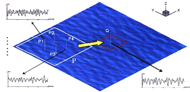
We define a right-handed Cartesian coordinate system o - xyz with the x- and
y-axes located on the mean free surface and the z-axis positive upward, as shown in Figure 2-1. Referring to this coordinate system, the problem of wave reconstruction and forecasting can be mathematically described as follows: given the probe data of wave elevation i(x, t), where x = (x, y), at specified locations x=x,,, n=l,..., N, for a limited period of time t E [0, T], using a wave model to construct a wave-field TI(x, t) in the domain P(x, t) such that
I](x-, t) =i (xpn, t) for tE [0,T] , n = 1, ... , Np. (2.1) As the wave-field in P(x, t) evolves, it will forecast the wave-field in the domain
Q(x, t) for t > T. In more general case, the probes can be mobile with controlled
paths, i.e., xP can be a function of t. 38
,YV Vmvv
Figure 2-1: Sketch of the wave reconstruction problem in a directional ocean wave-field.
2.3
Basic assumptions
For deterministic wave reconstruction and forecasting based on wave probe measure-ments, we make the following assumptions:
" the wave energy spectrum is assumed limited in both frequency band and di-rection spreading; no assumption is made about the stationarity or the homo-geneity of the spectrum; and no information about the shape of the spectrum is assumed because all the statistic information can be obtained from the probe measurements.
" the flow is assumed to be a nonlinear potential flow with wind input, viscosity, and bottom friction effects neglected; effects of finite water depth, ambient current, and wave breaking are taken into account.
" the probe measurements are assumed perfect, noise-free. To study the effect of measurements noise on the wave reconstruction and forecasting, we use a
Monte-Carlo simulation method in Chapter 6. 39
PPP-2.4
Characteristics of ocean wave spectrum
To justify our assumption about the wave spectrum, we now study the characteristics of ocean wave spectrum.
Ocean waves have long been measured and analyzed using statistics. Based on many time records, the frequency spectrum of ocean waves can be obtained. There-fore, frequency spectrum is often used to describe the state of an ocean wave-field.
In 1955, Pierson et al. first introduced the wave energy spectrum, which can be defined as a function of frequency and direction. The energy spectrum of ocean waves cannot have arbitrary form; instead its form is decided by the physics involving wave generation, propagation, and breaking.
Pierson and Moskowitz (1964) proposed a frequency spectrum for a fully developed sea based on similarity theory and measurements as
S(w) = 0.0081g2W-5e-0.7494(UW)-4. (2.2)
Here S is the energy density, g the gravity, w the wave frequency, and U the wind speed measured at a height of 19.5 meters above the sea surface. This is called the P-M spectrum.
In 1973, a lot of ocean wave spectra was measured in the JONSWAP project and
it was realized that the spectrum of a growing sea has a much sharper peak than the
P-M spectrum. Therefore, a new spectrum was proposed:
(w- W)2
5( w -4 aw
S(w) = ag2 w-e- 4 e (2.3)
Here a = 0.0081, -y is the peak enhancement factor, and wo is the peak frequency.
o- = 0.07 when w < wo and 0.09 when w > wo. This is called the JONSWAP spectrum. Figure 2-2 shows the comparison between the P-M spectrum and the JONSWAP spectrum with wo = 0.52. The total energy of these two spectra are the same. From this figure we can see that the wave energy of long waves or short waves are very small and most of the wave energy is contained within a finite frequency band around the
S (O) 20 15 10 5 0-0 (m2s) 'I Ii Ii Ii Ii I' I ~ I ~ 1\ I I I 0.5 1 1.5 co (rad/s) 2
Figure 2-2: P-M spectrum and JONSWAP spectrum.
w1 W2 E(wi,w2)/Eo
0.39 0.83 80% 0.37 0.99 90% 0.35 1.17 95% 0.33 1.72 99%
Table 2.1: P-M spectrum energy distribution.
dominant frequency, which corresponds to the peak of the spectrum. For JONSWAP, it is more obvious. To see it more clearly, we define the energy within a frequency
band [w1, w2] as
IW2
E(w,,W2) Lif S(w)dw.
Then the total energy can be written EO = E(0, oc). In Table 2.1 and Table 2.2 we
showed the ratio between E(wi, w2) and EO for some frequency bands
[w
1, w2] for theP-M spectrum and the JONSWAP spectrum.
From these tables we can see that more than 95% of wave energy is contained within a frequency band of 0.7 ~ 0.8 rad/s, although the wave spectrum itself extends