DISTRIBUTED PARAMETER ACTIVE VIBRATION CONTROL OF SMART STRUCTURES
by Scott E. Miller
S.B., Massachusetts Institute of Technology (1986)
SUBMITTED TO THE DEPARTMENT OF MECHANICAL ENGINEERING IN PARTIAL FULFILLMENT OF THE REQUIREMENTS
FOR THE DEGREE OF MASTER OF SCIENCE
IN
MECHANICAL ENGINEERING at the
MASSACHUSETTS INSTITUTE OF TECHNOLOGY
April 26, 1988 ( Scott E. Miller 1988
The author hereby grants to M.I.T. and the C.S. Draper Laboratory, Inc. permission to reproduce and to distribute copies of this thesis document in whole or in part.
Signature of Author
Department of Mechanical Engineering ,April 26, 1988 Certified by
Dr. James E. Ulkbbard, Jr. ThYsis SupervisorC,. E-Technical Staff Accepted by
Professor Ain A. Sonin Chairman, Department Thesis Committee
MASSWCHUSETTS INSTITU
F TFr/'4-'t .G0rV MAY 5 1988
UBRARIES
DISTRIBUTED PARAMETER ACTIVE VIBRATION CONTROL OF SMART STRUCTURES
by Scott E. Miller
submitted to the Department of Mechanical Engineering in partial fulfillment of the
requirements for the degree of Master of Science ABSTRACT
A vibration control strategy for multi-component structures has been developed in which the structural components are actively damped beam members. Each com-ponent is mart in the sense that it is an active vibration control system which is autonomous of all other structural components. Distributed sensor and actuator transducers constructed from polyvinylidene fluoride (PVF2) are embedded in each
beam element. Lyapunov's direct method was used to develop a vibration control strategy for a generalized system consisting of an arbitrary number of smart beam members rigidly joined at a common boundary. The analysis leads to a smart com-ponent control law which guarantees stability to the global system. The distributed transducer electric fields may be varied to provide controllability to all modes or to specific modal subsets of a structure. Guidelines are presented for choosing film electrode spatial distributions to meet design goals. A universal spatial film distri-bution is proposed which has the potential of providing active damping to all modes of many structures with nearly arbitrary boundary conditions.
To develop the control methodology, theoretical models for spatially distributed transducers on flexible beam components were derived. An analytical model for spatially distributed sensors on flexible beam elements was developed without the necessity of modeling the beam in terms of its component vibrational modes. The model provides insight into the observability of beams with nearly arbitrary bound-ary conditions. The sensor electrode surface may be spatially distributed so as to function similar to point sensors or to produce a signal in which certain vibrational modes of the structure are weighted more than others. A previously derived model for PVF2 actuators is presented in terms of its duality with the distributed
sen-sor analysis. The sensen-sor model was verified experimentally for spatially uniform and linearly-varying sensors applifed to a clamped-free beam. The signals provided by the distributed sensors were compared to the outputs of corresponding point sensors.
PVF2 sensors and actuators situated on the same structural component developed radiative noise problems which were effectively compensated with noise reduction circuitry.
Experimental results were obtained which validate the smart structure control strategy. A smart beam component was constructed, the component was can-tilevered, and controllability was demonstrated for the first two vibrational modes. A multi-component structure was then constructed from three rigidly joined au-tonomous smart components, and the smart structure control methodology was validated experimentally. Frequency and transient response data for the first four modes demonstrate that the smart structure control strategy is effective in providing active damping. A digital simulation using MSC-NASTRAN and CTRL-C yielded results which support the experimental analysis. The simulation demonstrates a methodology for modeling and analyzing smart structures.
Thesis Supervisor: Dr. James E. Hubbard, Jr.
Title: Lecturer of Mechanical Engineering, MIT C.S. Draper Laboratory Technical Staff
ACKNOWLEDGEMENT
This thesis is dedicated to Carole Stacy Berkowitz. in her brief life Carole brought warmth into the lives of many people: I feel fortunate to have been one of those individuals. She always strived to repair the many injustices that we face in our world, and so she chose to dedicate her life to helping the deaf and the emotionally ill. Carole had a gift of human understanding that has touched many. Carole will always be missed, and will be forever with me.
You are never given a dream without also given the power to make it true.
Completing my Masters degree at MIT is the fulfillment of a dream for me, and one that would not have been possible without the support of many truly caring people. My mother and father taught me as a child to pursue my dreams, and as an adult that sharing one's dreams with the people one loves is the essential element that makes life a joyful experience. My brother, Eric, is my friend as well, and I am thankful that we are close. Tamar Siegel, who has had to endure her share of neglect over the past few months as I have been laboring over my thesis, has always been a terrific provider of encouragement and support. Bob Litt and Fran Myman helped to pull me through some difficult times, and have proven themselves to be people I can always count on.
This thesis would not have materialized if not for the support of some extraor-dinary minds at Draper l.aboratory. I would like to thank Jim Hubbard for being my thesis advisor, and for putting his confidence in me to help me to grow both technically and individually. Alex Gruzen is a LATEX wizard, and has really helped to make Draper a pleasant environment for me. Tom Bailey has been an invaluable help to me over these past wo years, and to Tom I leave a thousand questions and all of my retired MORIA characters. Shawn Burke and John Connally have been excellent sources of good judgement at times when I wasn't: to both of them I leave all of my stability issues. There are a great many people both in and outside of Draper that must go unmentioned (or I may never finish this thesis), which I apologize for. You have all been invaluable.
I hereby assign my copyright of this thesis to The Charles Stark Draper Labora-tory, Inc., Cambridge, Massachusetts.
Scott Miller
Permission is hereby granted by The Charles Stark Draper Laboratory, Inc. to the Massachusetts Institute of Technology to reproduce any or all of this thesis.
TABLE OF CONTENTS
Section Page
1 Introduction ... 1
2 Theoretical Analysis of Smart Components ... 4
2.1 Distributed Sensing Using PVF2 Film ... 4
2.2 Distributed Actuation Using PVF2 Film ... 6
2.3 Derivation of Smart Component Control Law . ... 9
2.4 Spatial Shaping of PVF2 Transducers . ... 10
2.4.1 Application of Spatially Distributed Sensors ... 11
2.4.1.1 Uniform Sensor Distribution . ... 11
2.4.1.2 Linearly-varying Sensor Distribution ... 14
2.4.1.3 Other Spatially Varying Sensor Distributions . . . 15
2.4.2 Application of Spatially Distributed Actuators ... 18
3 Theoretical Analysis of Smart Structures . ... 20
3.1 Equations of Motion for a Generalized Structure . ... . 20
3.2 Smart Structures Control Strategy ... 26
3.3 Smart Component Spatial Distributions . ... 29
3.4 Design Guidelines for the Application of Smart Components .... 40
4 Experimental Analysis of Sensor Model . ... 42
4.1 Spatially Uniform Sensor on a Cantilever Beam . ... . 42
4.2 Linearly-varying Sensor on a Cantilever Beam . ... 47
4.3 Radiative Cross-coupling Between PVF2 Sensors and Actuators . . . 48
5 Experimental Anaiysis of Control Methods ... 56
5.1 Experimental Verification of Smc, Component Control Law . . . . 56
5.2 Experimental Verification of Smart Structures Concept ... 60
6 Smart Structures Computer Simulation ... . 75
6.1 Finite Element Model ... 75
6.2 Simulation of the Control Law Using CTRL-C ... 76
7 Conclusions and Recommendations ... 86
A NASTRAN Simulation Data ... .. 89
LIST OF FIGURES
Geometry of beam-film composite structure ...
Geometry of a smart structural component ...
Spatially uniform film distribution ...
Linearly varying film distribution. ...
Spatial sensor distribution for a clamp-clamped beam.. Spatial sensor distribution for a clamp-clamped beam.. Geometry of an arbitrary multi-component structure .. Two rigidly joined smart components ...
Choice for transducer distributions ...
Choice of transducer distributions ...
Choice of transducer distributions ...
Universal distribution
...
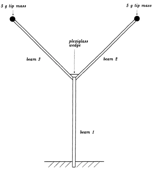
Top view of Y-structure
...
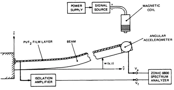
Experimental configuration for the uniform sensor analysis ...
Operational amplifier buffer circuit. ...
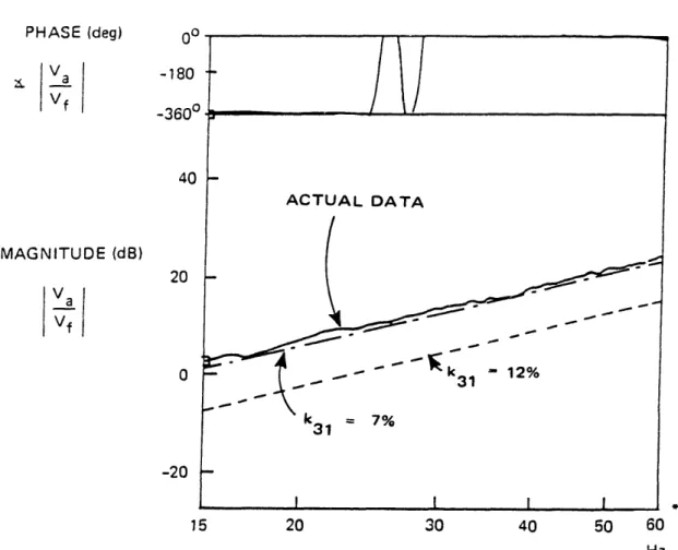
Uniform sensor distribution results, 15 to 60 Hz data... Linearly-varying sensor applied to a cantilever beam, side view.... Linearly-varying sensor distribution results.
Radiative cross-coupling phenomenon
Differential circuit to reduce cross-coupling effect.
Experimental configuration with cross-coupling rejection circuit in-cluded .
Experimental results with rejection circuitry included.
Frequency spectrum data for the cross-coupling experiment ...
Experimental configuration for control analysis. First mode results ...
Second mode results . ...
Geometry of Y-structure common junction.
vii Page 5 9 12 12 16 16 Figure 2-1 2-2 2-3 2-4 2-5 2-6 3-1 3-2 3-3 3-4 3-5 3-6 3-7 4-1 4-2 4-3 4-4 4-5 4-6 4-7 4-8 4-9 4-10 5-1 5-2 5-3 5-4
...
21
..
...
..
31
.... . .33
... .. 34 ... .. 36 ... 37...
..
39
43 44 46 49 49 51 52 53 54 55 57 58 59 62Experimental setup for the Y-structure control experiment. Analog compensation circuitry ...
Modeshape for the first bending mode of the Y-structure. . . First mode transient response data ...
Modeshape for the second bending mode of the Y-structure. Second mode frequency response data ...
Modeshape for the third bending mode of the Y-structure. Third mode frequency response data ...
Modeshape for the fourth bending mode of the Y-structure. Fourth mode frequency response data ...
Location of discrete sensor and actuator pairs ...
Magnitude Bode plots for the base beam ...
Phase Bode plots for the base beam ... Magnitude Bode plots for beam 2 ...
Phase Bode plots for the base beam ...
viii1 5-5 5-6 5-7 5-8 5-9 5-10 5-11 5-12 5-13 5-14 6-1 6-2 6-3 6-4 6-5 63 64 66 66 68 69 70 71 72 73
....
80
....
81
... .
82
... .
83
... .
84
LIST OF TABLES
Table
4-1 Uniform Sensor Analysis Experimental Parameters ...
4-2 Linearly-varying Sensor Analysis Parameters ... 5-1
5-2
5-3
Experimental Results for Component Control Analysis ...
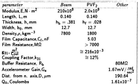
Y-structure Experimental Parameters ... Smart Structure Control Analysis Results ...
45 50 60 74 74 6-1 Modal Frequency Estimates. ... 85
ix
Chapter
1
Introduction
The component elements used in systems such as large space structures are typically light, flexible, and have a large number of vibrational modes. These modes are generally lightly damped. Mission requirements, such as weight constraints, often preclude the incorporation of passive damping treatments. As a result, interest has been generated in the past several years regarding the application of active control techniques to the vibration control of distributed systems [1]. Traditionally, active dampers used in this context have been based on the implementation of a finite number of discrete sensors and actuators [2,3,4,51. Since the flexible components are continuous and in theory possess an infinite number of degrees of freedom, these control schemes truncate the system model to a finite number of discrete modes [51.
It is often difficult to determine the number of modes required to accurately model the structure, and to reconcile the location of the sensors and actuators.
A research effort was initiated at MIT to apply a distributed actuator to the vibration control of a flexible beam [6,71. The active damper consisted of a layer of the piezoelectric polymer, polyvinylidene fluoride (PVF2). PVF2 is a polymer which
can be made piezoelectrically active through appropriate processing during manufac-ture. A voltage field applied across the faces of the film layer results in a longitudinal strain over its area. Analysis has shown that controllability for nearly arbitrary beam boundary configurations can be achieved by permitting the distributed actuator's control to vary in space as well as in time [1]. The results further indicate that for a broad class of boundary conditions, controllability can be achieved by producing an electric field across the distributed film actuatoe that is proportional to a unique feedback parameter [81.
CHAPTER 1. INTRODUCTION
The research study described herein was begun in part to design and construct distributed sensors using PVF2 film. The study emphasizes the versatility of film
sensors in particular applications relating to lightly damped beams, with the intention of showing how distributed sensors may be used in alternate applications. The use of PVF2 film as a sensor has been studied in applications that have included detecting tactile information for robotic endeffectors
[91,
utilizing PVF2 as a tactile stimulatorand mechanical transformer element in a reading aid for the blind [101, implementing piezoelectric film in high frequency audio speaker systems [11,12,13], and others [14].
In the area of elastic continua, some research has been completed in which general observability and controllability conditions for a flexible body have been developed.
it has been shown that in many cases, controllability and observability of all flexural modes can be achieved in theory with only one sensor and actuator pair co-located at a free boundary [15].
A model for the design and analysis of spatially distributed sensors is presented which shows that observability for nearly arbitrary beam configurations is possible
by utilizing distributed sensors whose strain field is caused to vary spatially. In this study PVF2 constitutes the active element: however, the analysis is applicable to
all candidate materials which behave in a distributed manner to produce an electric field from applied strain. The model was derived without the necessity of modelling the beam in terms of its component vibrational modes. The model shows that the sensor electrode layers can be spatially varied so as to produce signals similar to point sensors or signals in which certain vibrational modes are weighted more than others. Experimental results are presented which support the model for two separate spatially varying electrode distributions on a cantilever beam. The film sensors were compared to corresponding point sensors. Radiative cross-coupling effects between PVF2 sensors and actuators were investigated, and a simple compensation technique was devised which effectively eliminates adverse noise corruption.
The main intent of this research effort was to develop a vibration control strategy for multi-component flexible structures. The control methodology that has subse-quently been developed and presented herein utilizes distributed transducers in order to preserve the ability to simultaneously control all modes or a specified subset of modes. The distributed sensor and actuator models are combined with Lyapunov's
CHAPTER 1. INTRODUCTION
second method, leading to a control law for flexible beam components. These ac-tively controlled beam components are smart in the sense that all of the essential elements of the active damper are self-contained (the component is a beam/PVF 2
composite in which the control algorithm may be embedded on a microchip). A strategy is developed for the vibration control of a generalized structure consisting of an arbitrary number of smart structural members rigidly joined at a common boundary. The global system can be controlled by enforcing the component control law applied locally to each smart structural element. Lyapunov's second method is used to derive the multi-component structure control strategy. Enforcing the con-trol law guarantees the stability of the global system for any spatial distribution of the transducer strain fields. Guidelines are presented for choosing spatial distribu-tions to meet design goals. A "universal" smart component transducer electrode distribution is presented which has the character of providing active damping to all modes of a structure for many structural configurations.
Experimental results were obtained which validate the smart structure control strategy. A smart beam component was constructed, the component was can-tilevered, and controllability was demonstrated for the first two vibrational modes. A multi-component structure was then constructed from three rigidly joined au-tonomous smart components, and the smart structure control methodology was validated experimentally. Frequency and transient response data for the first four modes demonstrate that the smart structure control strategy is effective in providing active damping. The greatest increase in modal damping was observed at the sec-ond mode of the structure, for which the damping ratio was increased by a factor of 28.8. A digital simulation using MSC-NASTRAN and CTRL-C yielded results which support the experimental analysis. The simulation demonstrates a methodology for the computational modeling of smart structures.
Chapter 2
Theoretical Analysis of
Smart
Structural Components
2.1
Distributed Sensing Using PVF
2Film
For uniaxially polarized PVF2 film, a longitudinal strain induces an electric field
across its faces [161. The induced field may be varied spatially by shaping the electrode plating over the faces of the film or by varying the film's thickness [1].
Although in this study the active element is PVF2, the analysis assumes only that the
distributed sensor produces an electric field from longitudinal strain. The analysis is therefore applicable to other candidate materials.
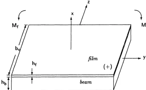
The geometric configuration of a beam/sensor composite is shown in Fig. 2-1. A PVF2 sensor layer is adhered to the top surface of a beam component. The film
polarity vector is oriented such that the positively charged surface of the film is the outermost surface. The strain induced on the outer face of the sensor film, Ef(y, ),
is a function of the curvature:
Ef(y,t) =
-D
2 77(2
-
1)
Oy2
where D is the distance from the neutral axis to the sensor film surface, is time, yq(y,t) is the elastic deflection of the neutral axis of the beam component parallel to the x-axis, and 82 is the curvature. The distance, D, is given by
D Ebh2 + Efh2 + 2Efhbhf hf
=
b+
2 f-
-- (2-2)(Ebhb + Efhf) 2
where Eb and Ef are the moduli of elasticity for the beam and film, and hb and hf are the thicknesses of the beam and film layers, respectively. Note that if the film
CHAPTER 2. THEORETICAL ANALYSIS OF SMART COMPONENTS
z
Mf
Y
hb
Figure 2-1. Geometry of a beam with a film transducer adhered to a single surface. thickness is much smaller than the beam thickness then
D hb
+hf
(2- 3)
2
The charge developed at a point on the surface of the sensor film is directly proportional to the longitudinal strain acting on the film at that point,
q(y,) =
(
k 31(y)(y)
(2
-
4)
where 2(y) is the distribution of the electric field parallel to the z- axis, k31 is the
electromechanical coupling factor, and g31 is a piezoelectric film constant ( )
The choice of the spatial weighting function, 2(y), may be enforced in a number of ways, such as varying the geometric shape of the electrode plating or altering the film thickness. The electromechanical coupling factor indicates the ability of the piezoelectric material to exchange mechanical energy for electrical energy, and is a function of both frequency and the quality of adhesion between the film and beam. It is assumed that the thickness of the electrode layer on the surface of the PVF2 film is negligible, so that spatially distributing the electrode plating does not
significantly change the stiffness of the PVF2 layer (electrode thickness is typically
on the order of 400A0 for Ni-AI plating on 28,/m film [161).
CHAPTER 2. THEORETICAL ANALYSIS OF SMART COMPONENTS 6
The total charge accumulated on the film surface, Q(i), is the spatial summation of all point charges, q(y, t), along the entire length of the electroplated film surface,
L: L
Q(j)
,/ q(y,i)dy
=
(2
-
5)
Combining Eq.'s (2-1), (2-4), and (2-5) gives
)(i)
g3=
)
a2D
07(y,
)
2(y)dy
(2 - 6)
It is preferable to nondimensionalize i(y) with respect to the width of the beam, b,, so that
2(y)
A(y) = --- y (2-
)
bo
where A(y) represents a nondimensional spatial distribution function. By considering the capacitive effects of the film as a dielectric material and combining Eq.'s (2-6) and (2-7), a relation for the film sensor output voltage, Vf, is obtained:
vf()=-Qc / afc-y1
-A(y)dy
.(2-8)
Eq. (2-8) is the governing distributed parameter sensor r ion. Cf is the film
capacitance. The constitutive charge coefficient, Qo, has units of Coulombs and is defined in terms of the pertinent piezoelectric and geometric constants:
Qo b k31D (2 - 9)
g31
The central concepts which generated the model were the strain-curvature relation-ship for a beam in bending and the applicable piezoelectric relationrelation-ship between
. longitudinal strain-and charge developed on the film surface.
2.2
Distributed Actuation Using PVF
2Film
The flexural vibrations of an elastic beam compone... having a PVF2 actuation
layer bonded to one face (see Fig. 2-1) have been described by Bailey [6]:
a
2[E ae
mV(y,)]
+pL
(210)
8yl MO-A = ; 0 < y < L (2 - 10)
CHAPTER 2. THEORETICAL ANALYSIS OF SMART COMPONENTS where
pA = pbAb + pfAf
(2-11)
El = EbIb + EfIf
(2-12)
EbEfhbbom
= -d31(hb +
hf)
2(Eh + Efhf)
(2-13)
In the above expressions r/(y,j) is transverse displacement, d31 is a piezoelectric constant, hb is the beam thickness, hf is the thickness of the film layer, and bo is the beam width. Bailey implicitly assumed throughout his analysis that the polarity vector of tie film layer was oriented such that the positively biased surface of the film actuator was the outermost surface. The linear inhomogeneous equation (Eq. (2-10)) is the Bernoulli-Euler beam model with a bending moment term, m.V(y, ), that results from the distributed action of the PVF2 actuation layer. The control moment
is as characterized a constant, m, which depends on the constitutive geometric, material, and piezoelectric properties of the composite structure and expresses the applied bnding moment per volt. The actuation layer may be spatially varied in order to weight the function of the distributed moment, as is described in 18]. Eq. (2-10) may be non-dimensionalized for convenience, giving
04w
2w
2V
y
4+
2
=< Y < 1
(2 - 14)
where the non-dimensionalized variables have the following definitions:
Y
=
y- (2-15) w = ? (2-16) LmL
V = El V (2-17)t
t(p--)
(2-18)
Eq. (2-14) may be used to determine the complete response of a particular sys-tem when combined with the appropriate set of boundary conditions. However the present form of Eq. (2-14) is ideally suited for investigating the behavior of
CHAPTER 2. THEORETICAL ANALYSIS OF SMART COMPONENTS
distributed actuation. The application of spatially varying actuator (and sensor) distributions is discussed in section 2.4.
A distributed parameter control algorithm was derived by Bailey [21,61 and Burke [8] using the second, or direct method of Lyapunov [23j. A Lyapunov func-tional was chosen that represents the sum of the beam's strain potential and kinetic
energies:
F=1
[ay
2
w
+ -
dY
(2-19)
Deriving the control algorithm using the Lyapunov functional in Eq. (2-19) allows for vibration damping to be implemented based on total system energy considerations and avoids the truncation of the system model. Burke showed that for a nearly arbitrary combination of boundary conditions for a given beam element, the time derivative of the Lyapunov functional (Eq. (2-19)) may be combined with the system governing equation (Eq. (2-14)) and written in the following form [81:
dF ' ar3w (Yt)dYwn(w
w
2dt
o
a2t
V(Y,
t)dY
+
fcn
t)
-(-
yt,
t),f(t),g(t))
(2 - 20)
where ~ represents the boundary point Y = 0 or Y = 1, and f(t) and g(t) are arbitrary forcing terms. The (normalized) control voltage to the actuation film, V(Y,t), appears only in the spatial integral term. In order to insure that energy is always removed from the system, V(Y, t) must be chosen to force the spatial integral term in Eq. (2-20) to always be negative. The control voltage may be written as the superposition of a control input time function, p(t), and a spatial distribution function, A(Y), such that
V(Y, t) = VoA(Y)p(t)
(2 - 21)
where Vo is the gain of the control signal. If the boundary terms are ignored in Eq. (2-20) and Eq. (2-20) is combined with Eq. (2-21), then
dF
I
1
a3w
d
= VOp(t) / ay2a A(Y)dY
(2 - 22)
This result will be combined in the next section with the distributed sensor relation-ship (Eq. (2-8)) in order to formulate a generalized control law for smart structural components.
CIHAPTER 2. THEORETICAL ANALYSIS OF SMART COMPONENTS z Mf
a
Mf
actuator(+)
hb beaensor (+)
Figure 2-2. Geometry of a smart structural component.
2.3
Derivation of Smart Component Control Law
Specific constraints regarding the geometry of smart structural components must be rigidly obeyed in order to give validity to the control law presented in this section. In a smart component two distinctly separate layers of piezoelectric film are adhered to both faces of a flexible beam element as shown in Fig. 2-2. In this study PVF2 is
used as the candidate material, but the analysis lends itself to any material which can function in a distributed way to produce charge proportional to strain or induce strain due to an electric field applied across its faces. One film layer acts as a sensor and the other as an actuator. Both film layers must be oriented such that the polarity of each layer is positively biased on the outer surface and negatively biased on the inner surface. In this way the sign convention presented hereafter in the control law derivation is maintained. It is further assumed that both film distributions maintain identical spatial geometries. Regardless of what shape is chosen for a particular application, it is essential that both the sensor and actuator distributions are of the same shape. Finally, the sensor and actuator pair must be co-located on the structure so that the smart component is symmetrical along the y-z plane as shown in Fig. 2-2.
The distributed sensor model (Eq. (2-8)) may be non-dimensionalized in terms
CHAPTER 2. THEORETICAL ANALYSIS OF SMART COMPONENTS 10
of the new variable set described in Eq. (2-15), giving
Vf(t) =
-| 1 a 2 w(Y, t)A(Y)dY
(2-23)
where Vf = Vf o is the nondimensionalized film sensor voltage. If the control signal time function, p(t), in Eq. (2-22) is defined to be proportional to the time derivative of the sensor film output such that
p(t) = dVf (2 - 24)
dt
then the time derivative of the Lyapunov functional, Eq. (2-22), becomes
dF
-=v0
[ jY2t
0,WA(Y)dY]
(2
-
25)
Eq. (2-25) is a major result which validates the smart component control law given in Eq. (2-24). Eq. (2-25) is always non-positive, indicating that enforcing the control law (Eq. (2-24)) guarantees that energy will be removed from the system. The linear control law insures stability but does not optimize the amount of energy extracted from the system. The control law is applicable to any choice of spatially shaped film distributions, provided that the actuator and sensor distributions are identical and co-located. The control law insures that any film shape will provide controllability to the system; however, the character and effectiveness of the con-troller will ultimately be determined by the spatial distribution (see section 2.4). Similarly stability is insured, in the sense that if Eq. (2-24) is obeyed then energy can not be added to the system. A poor choice in a transducer shape may result in no active energy dissipation for certain vibrational modes, but will not provide excitation to those modes. The control law derivation has not required a modal analysis of the dynamic system; hence, the results are applicable to broad class of beams with nearly arbitrary boundary constraints.
2.4
Spatial Shaping of PVF
2Transducers
In this section, theoretical results are presented which show that by spatially varying the electric field of the PVF2 sensor and actuator layers, specific modal
CHAPTER 2. THEORETICAL ANALYSIS OF SMART COMPONENTS
subsets of an arbitrary beam system can be selectively controlled or all modes can be controlled simultaneously. A detailed treatment of spatially varying distributed sensors will be presented first, and analogies will then be made which link the behavior of spatially shaped sensors to the behavior of spatially shaped actuators.
2.4.1
Application of Spatially Distributed Sensors
The electric fields of distributed PVF2 sensors and actuators may be varied so as to sense a distributed parameter or provide pure distributed actuation. PVF2
trans-ducer shapes may be carefully chosen in order to induce response functions similar to discrete transducers. Certain PVF2 sensors can be described as measuring point
angular and linear displacements, while similar PVF2 actuators can be modeled as
generating concentrated moments and forces. This representation is easily accom-plished through the use of generalized functions, which are a notational restatement of singularity functions [17]. The generalized step function, h(Y - a), is equal to zero for all Y < a and equal to unity for all Y > a. Throughout the ensuing analysis it is assumed that distributed transducer electric fields are caused to vary by spa-tially shaping the electrode plating on the film surface. A spaspa-tially uniform electrode distribution which extends along the entire beam surface is denoted as
A(Y) =
h(Y)- h(Y - 1)
.
(2
-
26)
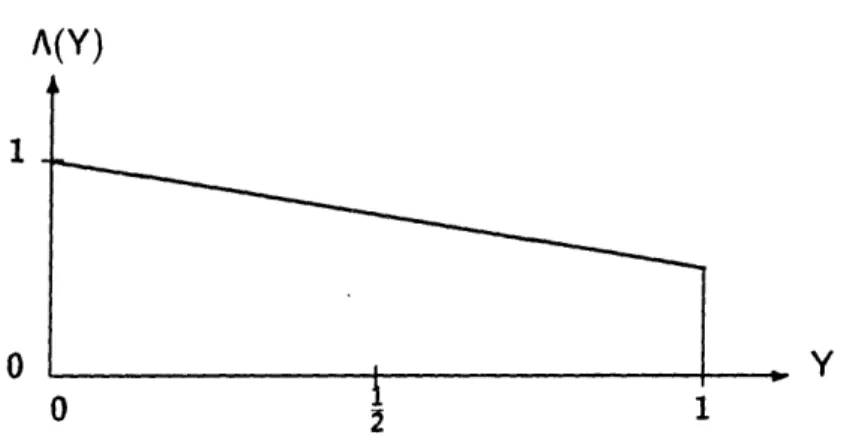
Similarly a "linearly-varying" electrode distribution extending along the entire length of the beam is written as
A(Y) = (1- Y) [h(Y) - h(Y-1)] . (2 - 27) Both distributions are illustrated in Fig.'s 2-3 and 2-4.
2.4.1.1 Uniform Sensor Distribution
If the uniform distribution (Eq. (2-26)) is applied to the sensor mooei (Eq (2-23)) and the integral is solved, the result is
Vf(t)
=
[aY
(O,t) - ay(1 t)]
(2
-
28)
THEORETICAL ANALYSIS OF SMART COMPONENTS
A(Y)
1
0
0
i
2Figure 2-3. Spatially uniform film distribution.
A(Y)
1
0
0
I
Figure 2-4. Linearly varying film distribution.
Y 1 Y I S p
CHAPTER 2.
12 IiCHAPTER 2. THEORETICAL ANALYSIS OF SMART COMPONENTS
This result has been arrived at based on the underlying assumption that the strain-curvature relation (Eq. (2-1)) is valid and the governing relation (Eq. (2-23)) is integrable along the entire domain. If boundary constraints are such that both
aY(0,t) and "y(1,t) are equivalent (e.g. clamp-clamped boundaries), then the uniform sensor distribution will fail to induce charge on the film surface. If the beam is clamped at Y = 0 and free at Y = 1, then the sensor will observe angular displacement at the free end, (1, t).
Spatially uniform sensors can observe all modes of any beam configuration in which one boundary is either clamped or sliding and the opposing boundary is either pinned or free. For a cantilever beam every mode is characterized by a nonzero angular displacement at the free boundary, and therefore every mode gives a positive contribution to the sensor output. In this sense all modes are observable. The output of a spatially uniform sensor will always be a measurement of angular displacement.
In a clamp-clamped configuration, however, both aw(,t) and w(1,t) are always equivalent and equal to zero, so that all modes are unobservable. Similarly a clamp-sliding configuration produces no sensor output.
An analysis of a uniform sensor on a pin-pinned beam lends insight into how distributed sensors function. The mode shapes of a pin-pinned (simply supported) beam are sinusoidal. Odd order modes exhibit even symmetry about the midspan, while for even modes the opposite is true. With all odd order modes, aw(0,t) -a(1,t, t),the integral in Eq. (2-23) is nonvanishing and thus all odd order modes are observable. For even modes aw(0,t) = aw(1,t), the integral in Eq. (2-23) vanishes and the uniform sensor is ineffective. The uniform nsor distribution may be represented as essentially half of a square wave in space and may be described in terms of a Fourier sine series containing only odd harmonics:
4
sin((2n + 1)rY)
(2-29)
Y7r
n=O=
2n +1
The modes of a simply supported beam are sine functions,
00
w(Y,t)
=
Esin(mwrY)q(t).
(2 - 30)
m=O
If the two preceding equations are appropriately included in the sensor relation 13
CHAPTER 2. THEORETICAL ANALYSIS OF SMART COMPONENTS
(Eq. (2-23)), then the resulting constitutive relation nearly becomes a restatement of modal orthogonality for odd order modes of the pin-pinned beam. All even values for the mode number, m, cause the integral in Eq. (2-23) to be zero, since these even modes are orthogonal to every spatial harmonic in the Fourier decomposition of the uniformly distributed sensor.
2.4.1.2 Linearly-varying Sensor Distribution
If the linearly-varying distribution (Eq. (2-27)) is applied to the governing equa-tion (Eq. (2-23)) and the integral is solved, then for all admissible curvatures the result is
Vf(t)
=
(a
(O,t) + w(O,
t) - w(1 t))
.(2 - 31)
The preceding equation reveals in part the significance of applying spatially varying sensors to certain beam configurations. Whereas the spatially uniform sensor cannot sense motion in a clamped-sliding beam, the linearly-varying sensor can: all modes become observable in the sense that each mode contributes a nonzero linear tip displacement at the sliding boundary.In the case of the pin-pinned beam, the linearly-varying film distribution de-scribed in Eq. (2-27) may be used to effectively observe all structural modes. When the boundary constraints are applied to Eq. (2-39), the linear displacement terms vanish and only the angular displacement term at the Y = 0 boundary remains. A Fourier decomposition of this distribution would include all of the sin(mirY) mode shapes. By replacing A(Y) in the sensor governing equation (Eq. (2-23)) with the Fourier series of the ramp functional, the result would essentially be a restatement of orthogonality for both odd and even modes of the pin-pinned beam. With the uniform distribution the angular displacements at both boundaries are equivalent for even modes and cancel each other in Eq. (2-28). The linearly-varying distribution eliminates this effect and allows for all modes to be observable in the sense that the charge induc.Ed or the film will be the sum of nonzero contributions from all modes. The linearly-varying sensor analysis reveals some unique features of spatially varying the sensor within the framework of generalized functions. Discontinuous
step changes result in the sensing of angular displacements and discontinuous slope 14
CHAPTER 2. THEORETICAL ANALYSIS OF SMART COMPONENTS
changes result in the sensing of linear displacements. The uniform film distribution (Eq. (2-26)) on a cantilever beam senses angular displacement at the free end, whereas the linearly-varying distribution (Eq. (2-27)) applied to a cantilevr beam clamped at Y=O senses linear displacement at Y=1. Distributed sensors act as discrete sensors when in these configurations, provided that the beam curvature is admissible in the sense that the linear strain-curvature relationship (Eq. (2-1)) is applicable.
2.4.1.3 Other Spatially Varying Sensor Distributions
In this section, spatially varying sensor distributions that are neither uniform nor linearly-varying will be considered. The preceding discussion lends insight into how a distributed sensor may function comparatively with a point displacement sensor. Uniform and linearly-varying distributions may be applied to a broad class of boundary configurations to produce an output parameter which is the sum of contributions from even, odd, or both even and odd modes of the beam. Furthermore it is possible to synthesize spatial sensor distributions that will weight the angular displacement measurement more than the linear displacement measurement, or vice versa. The result may be a sensor signal that is more sensitive to odd modes than to even modes, etc., depending on the particular beam/sensor configuration.
The clamp-clamped beam provides an interesting example. A clamp-clamped beam will have modes with either a vanishing displacement or a vanishing slope at the midspan, but never both. Using insights gained from the previous analysis, an appropriate film distribution which senses contributions from all vibrational modes can be found. A spatial distribution with a discontinuous amplitude (step) change and slope change at the midspan will provide observability, and the magnitude of either the step or slope change may be varied to weight certain modes more than others. The spatial distributions in Fig.'s 2-5 and 2-6 have both step and slope
changes at Y = . However, the magnitude of the slope change in the former figure is twice that of the latter: thus in Fig. 2-5 odd modes are weighted twice as heavily as even modes relative to Fig. 2-6.
In certain applications it may be advantageous to resort to distributions which 15
CHAPTER 2. THEORETICAL ANALYSIS OF SMART COMPONENTS A(Y) 1 0 0 Y 1
Figure 2-5. Spatial sensor distribution for a clamp-clamped beam.
A(Y) 1
i
0 0 12 Y 1Figure 2-6. Spatial sensor distribution for a clamp-clamped beam.
g aim
CHAPTER 2. THEORETICAL ANALYSIS OF SMART COMPONENTS 17
have continuous slope changes that are non-uniform. An interesting example is that of sensing a single vibrational mode. Consider a beam configuration where the cur-vature relation corresponding to a particular mode has been determined analytically
or approximated through computational methods. For most beam systems it is often impractical to determine the curvature relation corresponding to a specific mode; however, the purpose of this section is merely to demonstrate a unique example in which a nonlinear film distribution may be applied.
For a beam which obeys the Bernoulli-Euler equation there are two principle statements of modal orthogonality. They are described mathematically as [181
/D kj(Y)1k(Y)dx = 6jk (2 - 32)
ID
j(Y>)1"'(Y)dx = 6jk (2 - 33)where oj(Y) and 4'k(Y) are eigenfunctions which correspond to the j and k modes
(the notation ()' indicates spatial differentiation), respectively, and
bj·k
{j 5-k
(2-34)
If Eq. (2-33) is integrated twice by parts, the result is
ID
i(Ok
it(Y)>
(Y)dx
(Y- [j(Y)'(Y
J (Y)'Ok Y --(Y y .D k(Y)]
D = = jk(2
-35)
Realizing that an admissible solution to the Bernoulli-Euler equation is a displace-ment field, w(Y,t), of the form
00
w(Y,t) = Ao
E
l/ni(Y)eiwt
(2
- 36)
m=1
and comparing Eq. (2-35) with Eq. (2-23), one observes that if A(Y) is chosen to vary spatially as the curvature, 0k"'(Y), of the k'th mode, then the sensor output will be proportional to the k'th mvde only, subject to the constraint
CHAPTER 2. THEORETICAL ANALYSIS OF SMART COMPONENTS
A pin-pinned beam is an example of a configuration which conforms to this
con-straint.
2.4.2 Application of Spatially Distributed Actuators
If the uniform film distribution, Eq. (2-26), is applied as a distributed actuator then the control input expression (Eq. (2-21)) becomes
V(Y, t) = Vo [h(Y)
-
h(Y
-
1)] p(t)
(2
-
38)
The control input appears in the governing actuator equation (Eq. (2-10)) in terms of its Laplacian due to the beam moment curvature constitutive equations. The effective loading that the uniformly distributed actuator presents to the beam is found by examining the Laplacian of Eq. (2-38), which is given by
02V
ay
2= Vo
['(Y)
- 6'(Y- 1)] p(t)
(2 - 39)
where the 6' terms are "doublet" or "concentrated point moment" functions. If the linearly varying distribution is applied as an actuator then the control input expression becomes
V(Y, t)
Vo(1 -
Y) [h(Y)
-
h(Y
-
1)] p(t)
(2
-
40)
for which the Laplacian is given by a2V
ay2
-V
[(Y) + 6(Y)
-
(Y
-
1)] p(t)
(2 -41)
where the terms represent "Dirac delta" or "concentrated point force" functions. A detailed treatment of PVF2 as a distributed actuator is presented by Burke [81, who rigorously shows that discontinuities in amplitude give rise to point moments,
while discontinuities in slope give rise to point forces. Prior studies have shown experimentally that the location of the discontinu;4ies can be varied so as to im-plement an actuator which will provide control to all modes or to a desired subset of modes [1]. Distributed actuator behavior is therefore analogous to that of dis-tributed sensors in the sense that PVF2 sensors observe angular displacements at
CHAPTER 2. THEORETICAL ANALYSIS OF SMART COMPONENTS 19
locations of amplitude discontinuities and linear displacements at locations of slope discontinuities. All of the theoretical observations made in the previous sections re-garding spatially shaped sensor distributions are applicable to distributed actuators as well.
Chapter 3
Theoretical Analysis of
Smart
Structures
3.1
Equations of Motion for
a
Generalized Structure
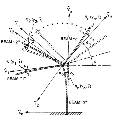
In this chapter the control law stated in Eq. (2-24) is applied in a general sense to a system constructed from an arbitrary arrangement of several smart structural elements. A generalized system is depicted in Fig. 3-1 in which an arbitrary number of smart components are rigidly joined to the free end of a cantilever beam. This system was chosen to facilitate an extension of the analysis which follows to a broad class of arbitrary structure geometries. The results of this chapter indicate that the energetic reactions between the component members will not degrade the stability of the actively controlled structure. The equations of motion are derived using Hamilton's Principle. Lyapunov's direct method is then applied to the system in conjunction with the distributed sensor and actuator models presented in the previous chapter to arrive at a control law for the generalized system.
Fig. 3-1 shows the geometry of the system. For convenience it is assumed that all beam components have a characteristic length, L. An inertial reference frame, designated as the XOYoZo frame is attached to the base of the cantilever beam.
Rotating reference frames are assigned to each of the elements that are rigidly con-nected to the free end of the cantilever. The frame associated with the j'th member is the designated as the xjyjzj frame. The yj unit vect.r is defined as tangent to the j'th element at the common junction, as show, in the figure. When the structure is at rest, the xjyjzj frame is rotated with respect t the inertial frame through the angle j in the Zo direction. The elastic deformation of the j'th element, 77j(yj,f),
is defined as the distance along a line perpendicular to the uyj-axis from any
CHAPTER 3. THEORETICAL ANAL SIS OF SMART STRUCTURES Yo 7r2 (Y2, t) Xnt'l ,,. 0 * * '71 yUt) VB1 "1" BEAM " 1 " x2
o(Yo t)
BEAM"O"Figure 3-1. Geometry of a superstructure formed from an arbitrary number of smart structural elements.
bitrary point pj on the uyj-axis to a point qj on the j'th smart component. For a system consisting of n components, a set of generalized coordinates which com-pletely specifies the system configuration at any instant of time can be expressed as
Ej=o0
7j(yj,t). This set of coordinates is completely independent since each coordi-nate can be arbitrarily varied while keeping all other coordicoordi-nates fixed. Not shown in the figure are arbitrary forces, fj(f), and arbitrary moments, gj(f), which may act at every boundary point yj = 1.To find the equations of motion it is first necessary to locate the point qj with
21
CHAPTER 3. THEORETICAL ANALYSIS OF SMART STRUCTURES 22
respect to the inertial frame. From Fig. 3-1,
Rqo Youyo + O70UXo (3 - 1)
and
Rqj
= LYo +
70o
y
+
yj
+
7Uxj
j
1,...,n
(3
-
2)
where 7L is defined as the translation of the 0'th component (i.e. the base beam) in the Xo direction at Yo = L. The velocities of the points qj with respect to the inertial frame are found by differentiating the displacement vectors:
-. dRq0 Vq - di 7/O0Xo (3 - 3) and dRq. dyi d.
Vqj = dt
-
LG
xYJ
+
+u/
d[
+(3 - 4)
di =t1- 1UXc+7 di . + di where j = 1, ..., n.The time derivative of a unit vector in a rotating frame is defined as the cross-product between the angular velocity of the frame with respect to the inertial refer-ence frame and the unit vector. Defining '0(t) as the slope of the base beam (beam "0") at Yo = L, i.e. (t) = (L,t), then the angular velocity of frame xjyjzj in inertial space is given by iu0ZO. Since the unit vectors Zo and 0z; in the inertial frame and in the xjyjzj frame, respectively, are equal,
d
=
x
xj
=
Y(3
-
5)
and
dO
-dt =
j
Yj
=
Ux;
(3-6)
The Xo vector can be expressed as the sum of components in uxj and iy'.
UXo
= sin(oj + k)uxj - cos(j + )yj
(3 - 7)
Combining Eq.'s (3-5), (3-6), and (3-7) with Eq. (3-4) yieldsCHAPTER 3. THEORETICAL ANALYSIS OF SMART STRUCTURES
The kinetic coenergy, T*, of the system is the sum of kinetic coenergy terms arising from each component beam member,
T =y
E
2mj
Vj *
Vjdyj
(3-9)
j=owhere mj = pjAj is the mass per unit length of the j'th beam, and torsional effects
of the beam have been ignored. Assuming small motions Eq.'s (3-3) and (3-8) may be inserted into Eq. (3-9) giving
T
=
2
o
02dyo
+
E{2
0
[7
-
27jyj
+
2±7Li7jsin(j + p)] dyj
J0oj
2y
i+
_ [1L3 +
L)L
2/Ltsin(5j +
I)]
}
(3-10)
where higher order terms (greater than 2nd order) have been neglected and terms not containing j(yj,t) were evaluated through the bounds of the integral.The total potential strain energy of the system, V, is determined based on the assumption that no shear strains are present, i.e. all structural members are modeled as Bernoulli-Euler beams. The total potential is given as
j=
L2
Jo
/Ab EbjyEj dAbjdyj + 2 A Ebjifj dAfjdyj (3- 11)where bj and ej are the axial strains of the beam and film layers, respectively, of the j'th component due to bending. Abj and Afj represent the cross-sectional areas of the beam and film layers of the j'th element; Ebj and Efj are the Young's Moduli pertaining to each element. Assuming small transverse displacements, the normal strains for the beam and film sublayers of the j'th component become
217j
Ebj = -xj a- say- (3 - 12)
and
efj = -X-y~4-
%
Eo
(3 - 13)
where xj is the distance in the uxj direction from the neutral axis to an arbitrary point within the beam/film composite. An initial prescribed prestrain, ,o, has been
CHAPTER 3. THEORETICAL ANALYSIS OF SMART STRUCTURES 24
added to the elastic strain of the film to account for strain induced through the piezoelectric effect. Combining Eq.'s (3-12) and (3-13) with Eq. (3-11) gives
V--I -j
)
dAbdyj
± [2 Eb+ ) dAfjdyjJ=O [
Joo
J(3- 14) The area moment of inertia of the j'th beam about its neutral axis is given by
Ibj
=
fA
xdAbj
(3
-
15)
bj
and similarly the area moment of inertia for the film layer is
= f| xzjdAf, (3 - 16)
The total moment induced on the j'th structural element due to the film, Mfj, is
M fj= f EfjeoxdAfj (3 - 17)
Af]
Eq. (3-14) may be combined with Eq.'s (3-15), (3-16), and (3-17) and reduced, giving the following expression for the strain energy of the system:
V=
{(J
[(El,)
(Y2 ) -
)2M7jyj2
dyj
+
Efie2dAfidyjj=0
2
y2
j
(3 - 18)
where (El)j = (EI)bj + (El)f.
The expressions for T* (Eq. (3-10)) and V (Eq. (3-18)) are used in conjunc-tion with Hamilton's Principle to arrive at the equaconjunc-tions of moconjunc-tion for the system.
Hamilton's Principle (Lagrange's Equation) is stated as
jt2 (T-
6V +
j(j)di
--
=
0
(3- 19)
where --j are nonconservative forces not represented in the expression for V. In this system it is assumed that arbitrary forces, fj(i), and arbitrary moments, gj(t), act on each element in the structure at the boundary point yj = L. When applying the
CHAPTER 3 THEORETICAL ANALYSIS OF SMART STRUCTURES 25
calculus of variations to the potential strain energy term it is essential to realize that both 6ti and 6t2 are equal to zero. The prescribed strain, co, is constant and can not be varied. The equations of motion are found by varying T' - V and integrating the result by parts in both spa. e and time until the independent variational variables are no longer in differential form. When integrating by parts the geometric boundary constraints at yj = 0 must be obeyed; namely, i7j(O,t) = 0j(O,t) = 0 for all j= 1, ..., n. The following system of governing equations are derived (j = 1, ..., n):
Beam 0: moio + (El)o
A1
4 =AM
2 (3-20)O4j + mjOL
sin(,~f
Beam
j:
mjj
+ (EI)j
a
t
-
mjy
j +
mjL
sin
+
)
(3-21)
The system is subject to the following natural boundary conditions at y = L:
E1
{
sin(*Jj + + ---.- m.o ,) mjj.in(*j + )dyi +(EI),o = M+
fo(T)(3
-22)
and- mj L3 m. L 2
,(omjL3
j sin(Oj+
+
- miyjijdy
i
+
(El)o
-
g3
( f
+
Y?
=
Mfo
+so(t)
(3-23)
The equations of motion also include two natural boundary constraints at yj = L
(i-= 1,...,n):
(El)j
= Mfj + gj(f) (3- 24) and 03rjaMfj
(El)ayj
yj
+fj()
(3-25)
Oyj3 OyjThe equations of motion have been derived based on the assumptions of small motions and the absence of shear strains. Eq.'s (3-21) through (3-25) may be nondimensionalized according to the following new set of variables for j=1,...,n:
J- L
CHAPTER 3. THEORETICAL ANALYSIS OF SAMART STRUCTURES
tj =
KjF
i
mjL4-MfjL
j
;
(EI)j
The system equations in
Equations of Motion:
82wo beam :at2
02wj beam j:
tnondimensional form are written as
4Wo a2 Mo
+
Oy4 =
a
2(3-26)
04 w__~
22Wo
a21~j
+
O
4- Ya
2 ++
sin(+
sin(
) at)82
(tj)=
aM
(3-27)
Natural Boundary Conditions at Yo = 1:
n 1
~~~2,.
s2 slll\~j + - 2w~·r _dv ,innj V~)-~.-
+
e2eao
m
2i'etj
-etJ
z'-'
n(j+ ) sd~j
+-tf=
it+fo(to)
j=Z J JO
j=j i i
,,2w
82W -Yd+ %2
'
+ = AO + go(to)wi YjdY - 4 i,(Oj + ) or.2
-
' ati J 2Jy i 0·1· · ·- 1· Natural Boundary Conditions at Yj = 1 (j = ,..., n):93wj
=
Ij Y3?
a-j
+fj(tj)
,9j
ayJ
02wj aV2 = IVlj + gj(tj) a3.2
Smart
Structures Control Strategy
In this section the smart structures control strategy is derived based on Lya-punov's second method [23]. Distributed actuator and sensor governing equations are combined with the Lyapunov functional time derivative to arrive at a smart
and n
j=l
(3 .- 28) ,t,/o'
I
O, -3 t (3 - 29) and(3
- 30)
(3 - 31) 26CHAPTER 3. THEORETICAL ANALYSIS OF SMART STRUCTURES
component control law which guarantees the controllability of the global system. It is assumed that the (undamped) generalized structure does not contain any unsta-ble modes. The (nondimensionalized) Lyapunov energy functional pertaining to the generalized structure is given as
1
2 2 ( )
F2
1
[(
(Yw
+
(8
dYo2
lo
0(
- ) 8YRj [Y)
+
,+
(Y*jj
+,,i(
ti,)
dYj.
(3-32)This functional is valid for small motions only: terms greater than second order have been neglected in order to be consistent with the assumptions made in deriving the equations of motion. The first and second terms in the first integral represent the potential strain and kinetic energies of the base beam, respectively. The first and second terms in the second integral represent the potential strain and kinetic energies of the j'th element. Differentiating the functional with respect to time gives an expression for the power in the system:
F=J_0 [ a yi.YOO+ -,,to
-"_
dYo'
+
E
{ Yj + sin(+jt
+)(l
-
+ sn(j +
(1)
t)
t)]
]
_ 0 a
+
"Y:j 2wj5
dYj
.(3-33)
+
i
The equations of motion (Eq.'s (3-26) and (3-27)) can be substituted into the above expression to replace the kinetic energy time derivative terms:
o 82w. o + - 4 dY +j - -Y*::(*% - " . y-4-y- dY
+
X
E
Yj + sin(-i +
) =;Ua
X
aa
j= J ' J (3-34) 27CHAPTER 3. THEORETICAL ANALYSIS OF SM,ART STRUCTURES
Differentiating both integrals by parts twice gives
F
=
101
o
MO+
3
MdYj
aw o O 03Wo Y| °
02Wo
02W
YO=1ato 8Y, aY3 ,V o,=o0 aYoat ay2 o0
+
F
ant
Yjat + sin(]j +
tj)
[1,
r)
aw=[·
atj
atj
OYJ2ayj[anj
ayYO
(
1 J Y=0
-
j
Otj
Wi
mi]
.
atj
J(3-35)
NA2
,
dtj 02w.1 Yy=iFinally Eq. (3-35) may be combined with the natural boundary constraints of the
system (Eq.'s (3-28)-(3-31)) to give the result
n 1 3w _ [ 2W. 02
w. 3w 1
F
= / 0 wjMjdYj +fcn
t J - ,tJ(, 'j(tj) ,tj)(tj),j=o
"
tJ j=O(3 - 36)
Eq. (3-36) shows that regardless of the energetic interactions between compo-nents in the large structure the moment induced by the film only appears in the spatial integral term. Recall that the (nondimensionalized) piezoelectrically induced moment is proportional to the (nondimensionalized) film voltage and varies in both space and time:
Mj = VojA(Yj)p(tj) (3 - 37)
where Voj is the gain of the control signal for the j'th component. Combining Eq. (3-37) with Eq. (3-36) and ignoring the boundary terms since they are independent of
Mj gives
VojPj(tj)] ay2tA(Yj)dYj (3 - 38)
j=o 10 0YJt
Tne film sensor governing equation for the j'th component fiows directly from Eq. (2-23):
()j=
-|
o
y2
(Yjtj) j(Yj) dYj
.
(3 - 39)
28CHAPTER 3. THEORETICAL ANALYSIS OF SMART STRUCTURES
In order to extract energy from the global system each structural component is
au-tonomouJly controlled according to the following control law for the j'th component:
pj(t)
=d
('f).
(3--40)
Applying Eq. (3-40) by differentiating Eq. (3-39) and substituting the result into Eq. (3-38) gives
l
=
E[Vojt
1 0wj
O~o
qn~,)~i,.
A(Yj)dYj
aw12
(3 - 41)
(3 - 41)
j=O
Eq. (3-41) shows that if each smart component is independently controlled ac-cording to the control law stated in Eq. (3-40) then the multi-component structure can not be destabilized since energy is always removed from the global system. Be-cause the negative definiteness of Eq. (3-41) the system is certain to be stabilizable, although the character and effectiveness of the global control strategy will ultimately be determined by the choice of spatial distributions and actuator orientations. It is important to note that at worst a poor choice in transducer shapes will render certain modes uncontrollable but will not provide excitation to these modes. It has
been assumed that all eigenvalues of the undamped structure are nonpositive. The result also implies that for systems of even greater complexity the same control law will still provide global stability. For instance, a system where an arbitrary num-ber of additional beams were rigidly joined to the free end of the n'th component (n
#/
0) of the current structure will lead to a new set of boundary terms at Yn = 1 to replace the fn(tn) and gn(tn) forcing functions. These terms will be similar to the natural boundary constraints that exist at Yo = 1 of the current system. New coupling terms will appear in the equations of motion that will also appear as kinetic energy terms in the Lyapunov functional: these terms will vanish in the final result through the substitution of the equations of motion into the Lyapunov functional time derivative.3.3
Smart Component Spatial Distributions
By choosing different PVF2 electrode spatial distributions for the component
members, it becomes possible to implement a controller that can control all modes
CHAPTER 3. THEORETICAL ANALYSIS OF SMART STRUCTURES
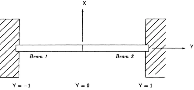
of a structure simultaneously or provide vibrational attenuation to a selected modal subset. In order to develop a methodology for choosing an effective combination of spatial distributions and actuator orientations, it is first necessary to approach a specific example system. Consider the simple structure shown in Fig 3-2, in which two smart components are rigidly joined at a common boundary and clamped at opposing ends. It is assumed that both components are characterized by the identical geometric and material constants. The specific constraints described in section 2.3 regarding the geometry and polarity of each component necessarily apply to this example system. The Lyapunov functional for the structure can be written as the superposition of functionals corresponding to each functional member:
fo {2w1Z
I-d
0Y2)
a(al2
dY
+ 1 (0a2a2)2
O(w
22dY
Taking the time derivative of the above expression yields
dF
o
2w,
0\
w
1awl
dY
ayf2I1 ay1
-t
&2
dt
-1\ y2 j\
2
y
\
tJ
\
at
f
{eW2
90
3W2
+
aw2
)
0
2w
2dY
Jol2)y2
J
yat)
at
at2
JJ
Eq. (3-43) is reduced by applying the equation of motion (Eq. (2-1, nate the transverse linear acceleration terms, integrating by parts, and boundary constraints. The resulting expression for ddF becomes
a{, dF
dt
J
o
(aOw V1dY+
l)V2dY93w -1 Oa2Yat \Yaat (3-43) 4)) to elimi-applying the (3 - 44)which is a restatement of the generalized expression (Eq. (3-36)) for this particular system. If the control input is restated according to Eq. (2-21) then
dF =
VolP1()
a2
3at AldY
+
Vo2P
2(t)fo (a
2at) A
2dY
dt
- 2Yo
(3 - 45)which is similar to Eq. (3-38).
Eq. (3-45) is suited for exploring various choices in smart component actuator shapes and global geometries. As a first case, consider the application of two smart
1