OF A CANTILEVER BEAM USING A
DISTRIBUTED-PARAMETER ACTUATOR
by
Thomas Lee Bailey
SUBMITTED TO THE DEPARTMENT OF MECHANICAL ENGINEERING
IN PARTIAL FULFILLMENT OF THE REQUIREMENTS FOR THE DEGREES OF
BACHELOR OF SCIENCE IN MECHANICAL ENGINEERING and
MASTER OF SCIENCE IN MECHANICAL ENGINEERING
at the
MASSACHUSETTS INSTITUTE OF TECHNOLOGY September 1984
Copyright 1984 Massachusetts Institute of Technology
Signature of Author r \v, i - /
Department of Mechanical' Engineering September, 1984 Certified by i.JJames E. Hubbard, Jr. Thesis Supervisor Accepte d by Warren M. Rohsenow Chairman, Department Thesis Committee
ARCHIVES
vASSACHUSET S itJSTTU E OF TEC(HNOLOG OCT 0 2 1984
3!-Distributed-Parameter Vibration Control of a Cantilever Beam using a Distributed-Parameter Actuator
by
Thomas Lee Bailey
Submitted to the Department of Mechanical Engineering on September 7, 1984 in partial fulfillment of the requirements for the degrees of Bachelor of Science and Master of Science in Mechanical Engineering.
Abstract
An active vibration damper for a cantilever beam was designed using a distributed-parameter actuator and distributed-parameter control theory. The distributed-parameter actuator was a piezoelectric polymer, poly(vinylidene fluoride). Lyapunov's second method for distributed-parameter systems was used to design a control algorithm for the damper. If the angular velocity of the tip of the beam is known, all modes of the beam can be controlled simultaneously. However, only the linear acceleration at the tip was measured, so the remaining analysis and the testing was done on a single mode at a time, up to the third mode. A simulation algorithm was developed to predict the effect of the active damper on the free decay of a single mode of vibration. A parameter study for the first mode was performed using varying control voltage limits and passive damping values.
Testing of the active damper was performed on the free decay of the first mode and with continuous excitation of both the first and second modes of the cantilever beam. A linear, constant-gain controller and a nonlinear constant-amplitude controller were compared in the free decay tests. The baseline damping of the first mode was ii=0.003 for large amplitude vibrations (2 cm tip displacement) decreasing to =0.001 for small vibrations (0.5 mm tip displacement). The constant-gain controller provided more than a factor of 2 increase in the modal damping with a feedback voltage limit of Vmx = 2 0 0 V rms. With the same voltage limit, the constant-amplitude controller achieved the same damping as the constant gain controller for large vibrations, but increased the damping by a factor of 40 to at least 1=0.040 for small vibration levels.
For the continuous excitation testing, the clamping fixture for the beam was mounted on a shaker. The beam was excited by bandlimited random noise that was
centered on the resonant frequency of interest so that only one mode of vibration would be present. Only the constant-gain controller was implemented for the continuous excitation tests. For the first mode, with the highest rms level of base acceleration and a control voltage limit of Vm =130 V rms, the loss factor was increased from a baseline damping of p=0.0040 to Tief=0.0054. With the lowest rms level of base acceleration and a control voltage limit of Vmx"=100 V rms, the damping was increased from rp=0.0026 to eff=0.020 . This corresponds to a 15 db reduction in the magnitude of the resonance. For the second mode, with the highest rms base acceleration and Vmax=2 5 V rms, the damping was increased from lp=0.0016 to Tieff=0.0 02 3 . For the lowest rms base acceleration and Vmax=30 V rms, the damping increased from lp=0.0014 to neff=0.003 9 . This is a 10 db reduction in the magnitude of the resonance.
Thesis Supervisor: James E. Hubbard, Jr.
Acknowledgements
I would like to thank my parents, Phillip and Darlene, for their unending physical and spiritual support. I would especially like to thank them for helping me to develop a very inquisitive nature and for passing along a good deal of 'common sense'. Little did they know that taking the time to deal with the multitude of questions from a young boy would someday lead to a degree from MIT.
I would also like to thank my wife, Beth. IHer love and support have never waivered during the past three years, even through the writing of this thesis. By providing a calm oasis away from the problems of school and research, she has helped to make MIT a much more enjoyable experience. I only hope that I can repay her for all the late evenings and weekends (weeks) of neglect.
Thanks to the others that have helped to make my stay here more enjoyable: Mr. Excitement and the other members of the Old Farts Club, Steve, Jon, Andrei, and all the
rest. Where would we be without friends?
Thanks to Shawn Burke for his technical help and analytical insight that often seemed to come at the most opportune moments.
I must also thank Jim Hubbard for his guidance and support throughout the past year. I greatly appreciate his faith in me and his friendship. My only regret from this thesis is that I didn't meet Jim sooner in my academic career.
Table of Contents
Abstract 2 Acknowledgements 4 Table of Contents 5 List of Figures 7 List of Tables 11 1. Introduction 12 1.1 Background 12 1.2 Objective of Research 132. Overview of the System 14
2.1 The Distributed Actuator 14
2.2 The Flexible Structure 15
2.3 The Active Damper Configuration 19
3. Theoretical Analysis 21
3.1 Modeling the Active Damper 21
3.2 Deriving a Distributed-Parameter Control Algorithm 26
3.3 Alternative Control Laws 29
3.4 Simulation of the Lyapunov Control Law for a Single Mode 30
3.4.1 The simulation algorithm 31
3.4.2 Bending strain energy as a function of tip displacement 31
3.4.3 Work done by the active damper 33
3.4.4 Energy dissapated by passive damping 35
3.4.5 Demonstrating the simulation algorithm 36
3.5 Parameter Study Results 40
4. Experimental Analysis 69
4.1 Construction of Scaled Test Structure and the Active Damper 69
4.1.1 Scaled Beam and Active Damper Construction 69
4.1.2 Fixture Construction 72
4.2 Stationary Fixture Tests 73
4.2.1 Measuring the Torque Constant 74
4.2.2 Impact Testing 76
4.2.3 Free Decay Testing 78
4.2.3.1 Apparatus and Procedures 78
4.2.3.2 Results and Discussion 79
4.3 Continuous Excitation Testing 89
4.3.1 Apparatus and Procedures 89
5. Conclusions and Recommendations 100
5.1 Conclusions 100
5.2 Recommendations 103
Appendix A. Equations of Motion For the Active Damper 105
A.1 Effect of the Piezoelectric Strain 105
A.2 Variational formulation of equations of motion 110
A.3 Non-dimensionalizing the equations of motion 113
Appendix B. Determining Mode Shapes 118
Appendix C. Dynamic Scaling of a Cantilever Beam 120
Appendix D. Effective Loss Factor from the Decay Envelope of a Free 128 Vibration
Appendix E. Distributed-Parameter Optimal Control for a Cantilever Beam 129
E.1 The Control Problem 129
E.2 The Cost Functional 131
E.3 Finding Canonical Equations 132
E.4 Forming the Distributed-Parameter Riccati Equation 138
E.5 Possible Weighting Matrices 142
E.6 Possible Problems with this Formulation 143
References14
List of Figures
Coordinate system for the PVF2.
Flexible test structure at the Charles Stark Draper Laboratory [11. Cantilever beam model of an arm of the Draper structure.
Active damper configuration. Active damper configuration.
The applied voltage produces a negative prestrain. Detail of composite beam cross section.
Several steps of a simulation.
Typical simulation results for free decay of first mode.
Figure 3-8: Tip displacement vs. time, decay envelope. loss factor varied.
Figure 3-7: Tip displacement. vs. time, decay envelope. loss factor varied.
Figure 3-8: Tip displacement vs. time, decay envelope. loss factor varied.
Figure 3-9: Tip displacement vs. time, decay envelope. loss factor varied.
V maz=4xlO 8. VMz=4xlO. 5 Vmaz=4x 10⁻⁴. Vm =8x10-malzz 4. Passive 44 Passive 44 Passive 45 Passi.e 45
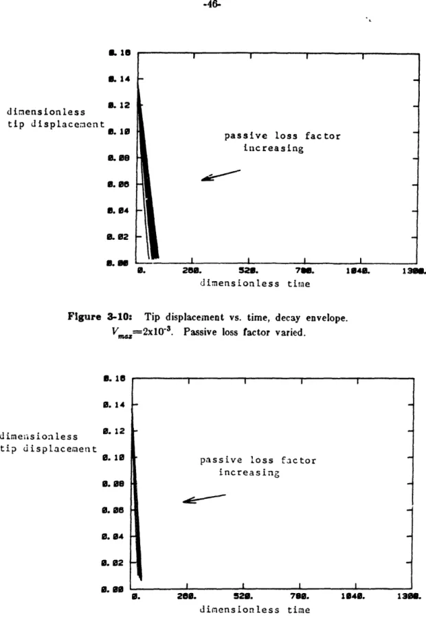
Figure 3-10: Tip displacement loss factor varied.
Figure 3-11: Tip displacement loss factor varied.
Figure 3-12: Tip displacement voltage varied.
Figure 3-13: Tip displacement voltage varied.
Figure 3-14: Tip displacement voltage varied.
Figure 3-15: Tip displacement voltage varied.
Figure 3-16: Tip displacement voltage varied.
vs. time, decay envelope.
vs. time, decay envelope.
vs. time, decay envelope.
vs. time, decay envelope.
vs. time, decay envelope.
vs time, decay envelope.
vs. time, decay envelope.
V =2x 10⁻³. V-,,=4x10O3. Tr=0.000 11p=0.001 qp=O.002 qp=0.003 np=0.005 Passive 46 Passive 46 Control 47 Control 47 Control 48 Control 48 Control 49 Figure Figure Figure Figure Figure Figure Figure Figure Figure 2-1: 2-2: 2-3: 2-4: 3-1: 3-2: 3-3: 3-4: 3-5: 14 17 18 20 22 24 32 39
Figure 3-17: Tip displacement voltage varied.
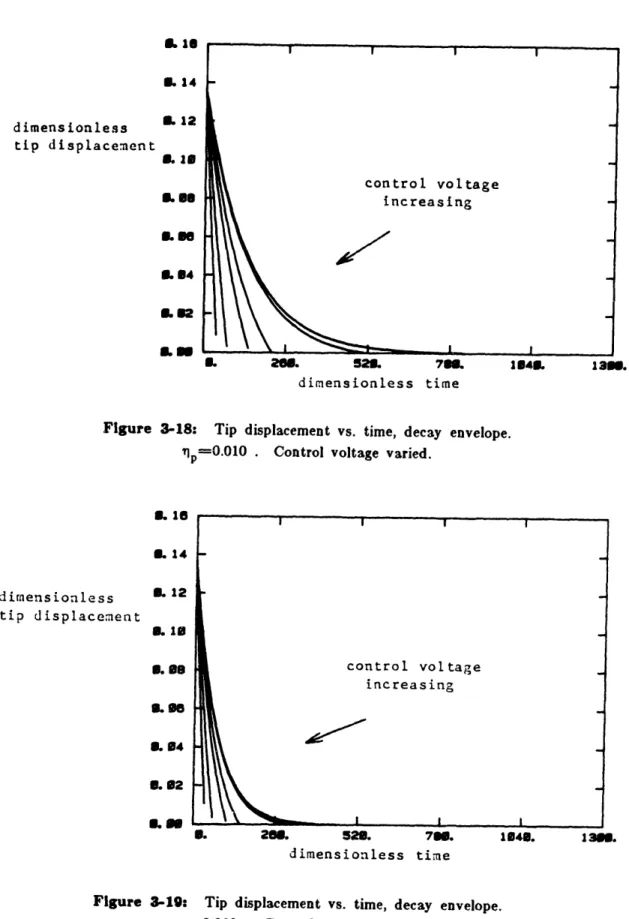
Figure 3-18: Tip displacement voltage varied.
Figure 3-19: Tip displacement voltage varied.
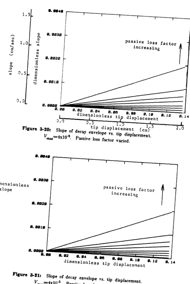
Figure 3-20: Slope of decay Passive loss factor varied.
Figure 3-21: Slope of decay Passive loss factor varied.
Figure 3-22: Slope of decay Passive loss factor varied.
Figure 3-23: Slope of decay Passive loss factor varied.
Figure 3-24: Slope of decay Passive loss factor varied.
Figure 3-25: Slope of decay Passive loss factor varied.
vs. time, decay envelope. ip=0.007 . Control
vs. time, decay envelope. ip=0.010 . Control
vs. time, decay envelope. p =0.020
V
.41
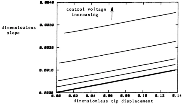
Control8envelope vs. tip displacement.
envelope envelope envelope envelope envelope vs. tip displacement. vs. tip displacement. vs. tip displacement. vs. tip displacement. vs. tip displacement.
"
-4x10
' 6V =4x10'
5.
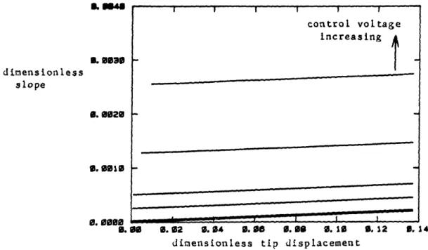
V =4x 10⁻⁵. Vm=8x10O-4. 1maOX10 3. V '=-1x10-fntlz 0-33. 49 50 50 53 53 54 54 55 55Figure 3-26: Slope of decay envelope vs. tip displacement. voltage varied. Figure 3-27: Slope of voltage varied. Figure 3-28: Slope of voltage varied. Figure 3-20: Slope of voltage varied.' Figure 3-30: Slope of voltage varied. Figure 3-31: Slope of voltage varied. Figure 3-32: Slope of voltage varied. Figure 3-33: Slope of voltage varied. Figure 3-34: Effective loss factor varied.
Figure 3-35: Effective
loss factor varied.
decay envelope vs. tip displacement.
decay envelope vs. tip displacement.
decay envelope vs. tip displacement.
decay envelope vs. tip displacement.
decay envelope vs. tip displacement.
decay envelope vs. tip displacement.
decay envelope vs. tip displacement.
p=0.000 p- =0.001 p pr =0.002 qp=0.00.3 Tp p=0.005 p-=0.007 p =0.010 Tp p=0.020
loss factor vs. tip displacement. Vmaz=4:;10-8
loss factor vs. tip displacement. Vma=4x10-5.V a--xl'S
Control 56 Control 56 Control 57 Control 57 Control 58 Control 58 Control 59 Control 59 Passive 62 Passive 62
Figure 3-38: Effective loss factor varied.
Figure 3-37: Effective loss factor varied.
Figure 3-38: Effective loss factor varied.
Figure 3-39: Effective loss factor varied.
Figure 3-40: Effective voltage varied. Figure 3-41: Effective voltage varied. Figure 3-42: Effective voltage varied. Figure 3-43: Effective voltage varied. Figure 3-44: Effective voltage varied. Figure 3-45: Effective voltage varied. Figure 3-48: Effective voltage varied. Figure 3-47: Effective voltage varied.
loss factor vs. tip displacement.
loss factor vs. tip displacement.
loss factor vs. tip displacement.
loss factor vs. tip displacement.
loss factor vs. tip displacement.
loss factor vs. tip displacement.
loss factor vs. tip displacement.
loss factor vs. tip displacement.
loss factor vs. tip displacement.
loss factor vs. tip displacement.
loss factor vs. tip displacement.
loss factor vs. tip displacement.
Vmaz =4x10⁻⁴. V =8x10- 4. V =2x10'3. Vm= 4x10O3. -=0.000 - =0.001 Ip=0.002 1p =0.003 ^p=0.005 ]p =0.007 p=0.010 qp=0.020 Passive 63 Passive 63 Passive 64 Passive 64 Control 65 Control 65 Control 66 Control 66 Control 67 Control 67 Control 68 Control 68 Figure 4-1: Figure 4-2:
Schematic of the active damper in stationary fixture. 70
Detail of tip mass. 71
Figure 4-3: Schematic of apparatus used to determine the effective torque constant.
Figure 4-4: Schematic of apparatus used for impact testing.
Figure 4-5: Typical transfer function from impact tests (first mode).
Figure 4-6: Schematic of apparatus used for free decay testing of the active damper.
Figure 4-7: Free decay of first mode results for the uncontrolled beam.
Figure 4-8: Free decay of first mode results for the constant-gain controller. V max =- 100 V rms.
Figure 4-0: Free decay of first mode results for the constant-gain controller. V max = 200 V rms. 75 76 77 78 82 83 84
Figure 4-10: Free decay of first mode results for the constant-amplitude controller. Vm&x = 100 V rms.
Figure 4-11: Free decay of first mode results for the constant-amplitude controller. Vm=X = 200 V rms.
Figure 4-12: Simulation results for the Lyapunov control law for two voltage limits. np = 0.002 .
Figure 4-13: Schematic of apparatus used for continuous excitation testing.
Figure 4-14: Continuous excitation testing, first mode, highest base acceleration.
Figure 4-15: Continuous excitation testing, first mode, medium base acceleration.
Figure 4-18: Continuous excitation testing, first mode, lowest base acceleration.
Figure 4-17: Continuous excitation testing, second mode, highest base acceleration.
Figure 4-18: Continuous excitation testing, second mode, medium base acceleration.
Figure 4-19: Continuous excitation testing, second mode, lowest base acceleration.
Figure A-1: Active damper configuration.
Figure A-2: The control voltage introduces a negative prestrain.
Figure A-3: Two layer beam in bending.
Figure C-: A cantilever beam with tip mass and tip inertia.
Figure D-1: An example of a free decay vibration.
Figure D-2: A free decay vibration plotted on a logarithmic scale.
85 86 88 89 94 95 96 97 98 99 105 106 108 121 126 127
List of Tables
Table 2-I: Table 2-II: Draper Table 3-I: Table 4-I: Table 4-II: Table 4-II1: Table B-I: Table C-I: Table C-II:Typical PVF2 film properties [2]. 16
Comparison of final design parameters for the scaled beam vs. the 19 structure.
Summary of Conditions for Parameter Study. 41
Parameters for the Active Damper. 73
Impact Test Results. 77
Summary of conditions for continuous excitation testing. 93 Eigenvalues and Predicted Natural Frequencies. 119 Possible choices for the scale model beam. 124 Final design parameters for the scaled beam. 125
Chapter 1
Introduction
1.1 Background
Satellites and other large spacecraft structures are generally lightly damped due to low structural damping in the materials used and the lack of other forms of damping, such as air drag. In large structures, these vibrations have long decay times which can lead to fatigue, instability, or other problems with the operation of the structure [1, 3. Flexible structures such as these are distributed-parameter systems having a theoretically infinite number of vibrational modes. Current design practice often is to model the system with a finite number of modes and to design a control system using lumped-parameter control theory. 'Truncating' the model may lead to performance tradeoffs when designing a control system for distributed-parameter systems 4].
Using distributed-parameter control theory to design the control system will avoid these tradeoffs by including all the vibrational modes in the design process and gives the potential for controlling all modes of vibration. There exists a wealth of distributed-parameter control theory in the literature, including the extension of many aspects of lumped-parameter control theory to distributed parameter systems. References [51 through [14] are a small sampling of the work being done. However, there are relatively few applications in the literature, especially for flexible mechanical systems. One reason may be the difficulty of using distributed-parameter control theory with spatially discrete, or lumped-parameter, sensors and actuators which introduce spatial non-linearities into the system. Distributed-parameter sensors and actuators would significantly ease the use of distributed-parameter control theory for flexible structures.
1.2 Objective of Research
The goal of this study is to design and evaluate an active vibration damper for distributed-parameter systems using a distributed-parameter actuator and to show some advantages of distributed-parameter control theory. The distributed-parameter actuator is a piezoelectric polymer, poly(vinylidene fluoride), or PVF2. At the Charles Stark Draper Laboratory, a scale model of a flexible satellite has been designed and built as a test structure for active vibration control schemes [1, 3. This test structure consists of a hub mounted on an air bearing table with four perpendicular arms extending radially from the hub. The arms rotate in a horizontal plane and are flexible laterally while being very stiff vertically. The active damper developed in this study will eventually be tested using the Draper structure. The damper is to be applied to the flexible arms. This thesis reports the development and preliminary testing of the active damper for the Draper test structure.
For the development work, an arm of the test structure was modeled as a cantilever beam with a tip mass and tip inertia. A smaller dynamically scaled model of one of the arms (including the use of a tip accelerometer) was used for the preliminary testing. Chapter 2 presents an overview of the system. The distributed-parameter actuator (PVF,), the Draper test structure and the dynamic scaling of the arm, and the active damper configuration are discussed. The theoretical analysis is presented in Chapter 3. The modeling of the active damper and the derivation of a distributed-parameter control algorithm are presented. Also a simulation algorithm is developed and a parameter study is performed. Chapter .1 presents the experimental work performed for the preliminary testing of the active damper. The construction of the test fixtures and the cantilever beam is discussed. The active damper was tested with the beam in a stationary fixture and in a vibrating fixture. The results from these tests are also presented and discussed. The final chapter summarizes the results of this study and presents some recommendations for further research.
Chapter 2
Overview of the System
2.1 The Distributed Actuator
The active element being used in this damper is a piezoelectric polymer film, poly(vinylidene fluoride), or PVF2. PVF, is a polymer that can be polarized, or made piezoelectrically active, by exposing it to intense electrical fields. In its non-polarized form, PVF2 is used as an electrical insulator, a capacitor dielectric material, and as a chemically inert coating, among many other uses. In its polarized form, PVF2 is essentially a tough, flexible piezoelectric crystal. Polarized PVF2 has been used in many applications ranging from ventilation fans [15, 161 to electroacoustic transducers (speaker and microphone elements) [17j to ultrasonic transducers for medical use [18J. More information on PVF2, other piezoelectric polymers, and their applications can be found in References [19] through [25].
A sketch of a piece of PVF2 film is shown in Figure 2-1. A layer of nickel or aluminum is generally deposited on each face to conduct the applied field or voltage, V(x), along the surface of the PVF2.
film
r(Vr ) on both faces
Figure 2-1: Coordinate system for the PVF2. ' '
a longitudinal (x-direction) strain. This is the d31 component of the piezoelectric activity. (Biaxially polarized PVF2 would strain in both the x- and z-directions.) The strain occ'lrs over the entire area of the PVF2 making it a distributed-parameter actuator. Note that if the voltage, V(x), is varied spatially, the strain will also vary spatially. This allows the added possibility of varying the control spatially as well as with time. The sign convention used in this study is that a positiv. voltage, as shown in Figure 2-1, results in a positive longitudinal strain.
The PVF2 used in this study was obtained from the Pennwalt Corporation, King of Prussia, PA. It is commercially available as a thin polymeric film with a coating of ni :kel or aluminum on its faces. Table 2-I gives some typical properties for Pennwalt's KynarTM brand PVF2 film 1[2.
2.2 The Flexible Structure
At the Charles Stark Draper Laboratory, a scale model of a flexible satellite has been designed and built as a test structure for active vibration control schemes 1, 3]. A sketch of the test structure is shown in Figure 2-2. This test structure consists of a hub mounted on an air bearing table with four perpendicular arms extending radially from the hub. The arms rotate in a horizontal plane and are flexible laterally while being very stiff vertically. This minimizes the effect of gravity on the motion of the structure. The arms are 1.2 m long and have either thrusters or weights for tip mass. The thrusters are mounted on one pair of opposing arms and are used to control the vibrations of the structure as well as perform attitude manuevers. Accelerometers at the tip of the arms are used to monitor the vibrations of the structure during and after the attitude manuevers. The damper developed in this study is to be applied to the flexible arms of the test structure to demonstrate the use of a distributed-parameter actuator for active control of a distributed-parameter system.
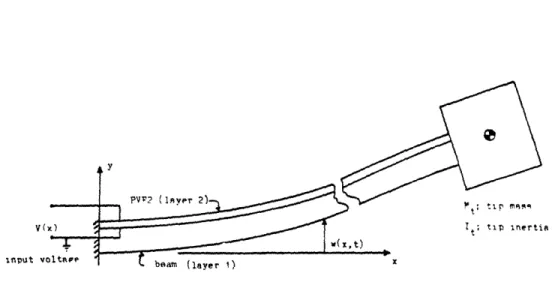
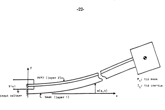
For the development work, an arm of the test structure was modeled as a cantilevered Bernoulli-Euler beam with both a tip mass and tip inertia (rotary inertia). A sketch of the top view of the cantilever beam model is shown in Figure 2-3. The nomenclature is as follows:
on the following page(s)
are not legible in the
original.
Table 2-I: Typical PVF2 film properties [21.
PROPERTY I VALUE UNITS
Thickness
!
6-125 mSurface Coanductivity1 A 1-4
nf IMetallized Film Ni 10-25
Static Piezelectric dt)-25 pCN- Ipni - I
Strain Constant * 0-22
Static Voltage g31 0.20 'mN
Output Coefficient . g 0.210 Electromech an<cali
Coupling actor : 9-15 , at 100 Hz
Pyroelectric Cotfficient p 23-27 uCm -'° OK '
Shrinkage n 60C 2 % after anailrng
Machine Direction 80oC 4 100 hi s.
Relative Dielectric
P ernm.Jtti. ; .I ' 12 -- 1 at 10(0 !iz Dielectric Lozs
Factor tan 6 0. .0i-J.u2 at 1000 Hz
Volume Resistivt P 10 .n Tensile Strength 1 Sm at ;e!d !" -i i I't.>:;;,: S:.': .:g'n ) , 2 at Break TD 3__-_ _ Elongation at I . D 4 Break TD 28-430 1bung's Iduu. of . ID 1.5 : Elasticity = E astic --- -N Strff!ess = c- TD 1 1-2.-4 Meiting P.,:::t i 63-180 : Flaninabrilitv. LO(I -44 ' 2 Thermal Cuiductivitv (J. 13 i W K
Specific Heat 2.5 NIJaf K
Density 1.8 g cn)
Therm::l E :p::., C,,¢!:'cic': I 10
iSound VlCILY: 1.5-2.2
'neasurement, \ ere rmadt :n hvdraulic pre- 'c- , -\11) -Machine D)rettv,n , I ad t'I'D TrIn- Icre 1fet l,,n t. film ,rlntatpn I2
RPL - EXPERIMENT TEST APPARATUS
CENTRAL HUB ASSEMBLY
(INCLUDES ANGLE ENCODER FUEL STORAGE TANKS)
\
-"ACTIVE BEAM TIP IINCLUDES TllnUSTEfS, ACCELEnOMETER AND VARIABLE MASS) AIn BEARING TABLE En .2 *J.
Figure 2-2: Flexible test structure at the Ch:arles Stark Draper Laboratory [1].
p is the density (mass per volume) of the beam E is the Young's modulus
I is the area moment of inertia of the cross-section about the neutral axis of the beam
I is the flexible length of the beam (x-direction) h is the thickness of the beam (y-direction) b is the depth of the beam (z-direction) Mt is the tip mass, and
It is the tip inertia taken about the z-axis at the end of the beam.
Note that the end of the beam is not necessarily the center of gravity of the tip mass. This study will only look at w(x,t), the transverse motion of the beam. The first step in the development of the damper was to dyamically scale an arm of the Draper structure to a more manageable size using the same techniques as Kelly used to design the structure
y
Ia
beoa
Figure 2-3: Cantilever beam model of an arm of -the Draper structure.
originally [1, 31. The scale model would also use an accelerometer at the tip of the beam to monitor the vibrations. The procedure used to scale the arm is given in Appendix C. The basic idea is to determine the dimensionless parameters that are used to describe the motion of the structure and then choose the physical parameters of the model so that the dimensionless parameters are preserved 1261. There are many possible combinations of physical parameters that will satisfy this criteria so some criteria other than just dynamic scaling must be used to chose a final design.
Other considerations in choosing the final design parameters for the scaled beam were:
1. The model size should be chosen so that the PVF2 film thickness would not be excessive when it is scaled and applied to the Draper test structure,
2. The scaled tip mass must be large enough to allow an accelerometer to be used as part of the tip mass, and
3. The beam should be easy to make and not have tight toler lices on the dimensions that are determined during construction.
The final design dimensions for the scaled beam are listed in Table 2-II along with the corresponding dimensions for an arm of the Draper structure. The beam material was chosen because it was found that steel feeler gauge stock was readily available in a wide range of
Table 2-II: Comparison of final design parameters for the scaled beam vs. the Draper structure.
Draper Scaled structure 11 model material Al steel modulus, E (Nm'2) 76x109 210x100 density, p (kgm-3) 2840 7800 length, I (m) 1.22 0.146 thickness, h (mm) 3.18 0.381 depth, b (cm) 15.2 1.27 tip mass, Mt (kg) 2.04 6.73x10⁻³ tip inertia, It (kgm2) 1.1x10⁻² 5.0x10⁻⁷
thicknesses, 1.27 cm depth (width), and up to 30 cm in length. Since the thickness of feeler gauge stock is held to a relatively tight dimensional tolerance, the most critical dimension of the scaled beam is already controlled. A thickness of 0.381 mm (0.015") was chosen. For this beam thickness dynamic scaling calls for a flexible length of 14.6 cm (5.766") and a tip mass of 6.73 g, more than adequate to include a 2 g accelerometer as part of the tip mass. Section 4.1 will discuss the actual construction of the scaled beam and the clamping fixtures.
2.3 The Active Damper Configuration
The simplest possible damper configuration was used for this study; a layer of PVF, bonded to one side of the cantilver beam. Figure 2-4 shows a top view of the resulting composite beam. The PVF2 is oriented as shown in Figure 2-1 so that a positive voltage across the film leads to a positive piezoelectric strain in the x-direction. It will be shown in Section 3.1 that this gives rise to a spatially distributed torque along the length of the beam. The resulting behavior is similar to that of bimetallic springs which coil and uncoil due to
Inpu '
Figure 2-4: Active damper configuration.
differential thermal expansion as the temperature changes. The basic understanding gained from this simple damper configuration can easily be applied to more complicated damper configurations such as PVF2 on both on both sides of the beam and/or multi-layer dampers that may include viscoelastic materials for added passive damping.
a
Chapter 3
Theoretical Analysis
This chapter describes the theoretical analysis performed to provide insight to the physical behaviour of the active damper. Section 3.1 describes the modeling of the active damper and the derivation and non-dimensionalization of the equations of motion. Section 3.2 presents the derivation of a distributed-parameter control law and Section 3.3 presents two additional control laws. Section 3.4 develops a simulation algorithm to predict the effectiveness of the active damper. Section 3.5 presents the results of a parameter study that was performed using the simulation algorithm. After the equations of motion have been non-dimensionalized in Section 3.1, the remaining analysis in this chapter is performed using dimensionless variables, unless otherwise stated. The results of the parameter study are presented in dimensionless form, although some representative plots also have dimensional axes that correspond to the scaled beam.
3.1 Modeling the Active Damper
The configuration of the active damper is shown in Figure 3-1. This is essentially a two layer cantilever beam. A subscript ()1 refers to the original cantilever beam while a subscript (')2 refers to the PVF2 layer. Only transverse vibrations of the beam, w(x,t, will be analyzed. The full equations of motion are derived in Appendix A. The derivation presented here is a summary and focuses on the effect of a voltage applied to the PVF.2
The effect of a voltage, V(x), applied an unbonded piece of PVF2 is to cause a strain, ep, in the PVF 2 which is given by
d31
p(,t) = V(x,t) · (3.1)
h2
where d31 is the appropriate static piezoelectric constant, h2 is the thickness (y-direction) of the PVF2 layer, and both are assumed to be uniform along the length of the PVF2. The PVF2 is assumed to be oriented so that a positive voltage yields a positive strain. When the PVF2 is bonded to the cantilever beam, this would be the equivalent of introducing a
1
input v
Figure 3-1: Active damper configuration.
negative prestrain, -Ep, in the PVF2 layer. The prestrain is negative because the PVF2 would strain p if it weren't bonded to the beam and it would take a prestrain of -ep to move the PV 2 back into place to be bonded. This is shown in Figure 3-2.
PVP, v I/// / // / / /// ._ .j pP 4-p Strain due to applied voltage. Prestrain needed to keep PVF2
the same length.
\ \ \ \
\ \ \ \\ \
Beam\
\ \\ \ \
Figure 3-2: The applied voltage produces a negative prestrain.
This prestrain has two effects on the beam. One effect is a longitudinal strain, el, to keep a force equillibrium in the axial (x) direction. The value of El can be found by solving the force equillibrium and is given by
I
I
IL
iiiq ... J. -E liB. I IE2h2
EXx,t) E = p(xt) (3.2)
Elhl+E2h2
where E is the modulus of elasticity and h is the thickness of the layers, again assumed to be uniform along the length of the active damper. The result of the prestrain and the longitudinal strain is a net force in each beam layer due to the applied voltage.
The other effect of the prestrain is that the net force in each layer acts through the moment arm from the midplane of the layer to the neutral axis of the composite beam, producing a torque, T(x,t), given by
T(x,t) = Elh lbE( - D + E2h2b( - p) h + 1 - D) (3.3) where b is the depth of the beam (assuming that bl=b 2) and D is the location of the
neutral axis of the composite beam, given by
Elhl2 + E2h22 + 2h h2E2
D = (3.4)
2(El1h + E2h2)
Figure 3-3 shows a detail of the cross-section of the composite beam. Substituting for the neutral axis in Eqn. (3.3) and reducing yields
EhlEh2b
( h +
2
T(x,t) (Eh + E ,h.) 2 (3.5)
Notice that all the terms involving El have been eliminated. This means that the torque depends only on the prestrain, not the longitudinal strain. Combining Eqns. (3.1) and (3.5) gives
ElhlE 2b
(
h + h2 )(Elh + E2h2) 2 dl Vxt)
c V(x,t) (3.6)
where c is a constant, for given beam materials and geometry, expressing the torque per volt. It is assumed that the material properties and geometry of the composite beam do not change along its length.
Combining Eqn. (3.6) with a conventional Bernoulli-Euler beam analysis yields the equations of motion for the transverse vibrations, w(x,t), for the composite beam. (See Appendix A for the derivation.) Assuming the longitudinal strain is negligible, the governing
Figure 3-3: Detail of composite beam cross section. equation is a4w a2w a2V(x,t) (3.7)
El -
+ pA -
- c-
for x: O<x<l
ax 4 at2 ax2 with boundary conditionsaw w = - = 0 for x=O ax a2w a3w
El -
= - I
+ c.V(x,t)
(3.8)
ax2 t2ax Sw a2w ~for x=--l a3w a2w av(x,t) El = M + c ax3 t at2 axwhere EI=E1I+EI 212, I is the area moment of inertia of the crosssection of the layer about the neutral axis, pA=plAl+p 2A2, p is the density of the layer, A is the cross-sectional area of the layer, I is the flexible length of the beam, and Mt and It are the tip mass and tip inertia, respectively.
These equations of motion can be non-dimensionalized to aid in scaling the analytical results from the scale model to the test structure and to provide insight into the important parameters of the system. The derivation in Appendix A suggests the following dimensionless variables.
x w W I /El cl
V
V
(3.9)
EI Mt Mt =- pAlIti
t
pAPUsing these dimensionless variables in Eqns. (3.7) and (3.8) gives the dimensionless equations of motion, which are
a4w a2w a2V(z,t)
+ -= for x: 0<x<l (3.10)
az4 at2 aZ2
with boundary conditions
3aw w = - = 0 for x--0 ax a2w a3w
-
-
I
t
=
fi
+ V(z,t)
(3.11)
ax2 at2az for z=1 a3 w a2w avIXt)M- +
For the development work, the simplest damper would have a uniform geometry and have a spatially uniform voltage applied along its length. For this configuration, the spatial derivatives of the input voltage are zero for the system described in Eqns. (3.10) and (3.11), leaving
a4w a2w
+ - = 0 for z 0<z<l (3.12)
axz at2
aw w = - = 0 for z=0 ax a2W a3w a2 I t t2 + V(t) (3.13) a3w a2W for z-l
= XM
Notice that the control voltage only appears in one of the boundary conditions. Therefore, Eqns. (3.12) and (3.13) describe a linear distributed-parameter system that has only boundary control. Since the actuator is a distributed-parameter actuator, the control was easily included in the equations of motion without nonlinear terms (e.q., spatial delta functions). This allows one to keep a linear distributed-parameter model throughout the analysis, avoiding any problems that may be caused by 'truncating' the model.
3.2 Deriving a Distributed-Parameter Control Algorithm
Distributed-parameter control theory was used to design a control algorithm for the active damper. This allows one the possibility of controlling all the modes of vibration at once, provided that the system is controllable through the actuator. Hence one may avoid problems with the spillover of the uncontrolled modes [4].
The control problem is to actively damp the vibrations of the system described by Eqns. (3.12) and (3.13) using the dimensionless input voltage, Vt), as the control variable. This dimensionless derivation can easily be converted to a dimensional formulation by substituting from the definitions of the dimensionless variables given in Eqn. (3.9). Assuming that there is some practical limit on the magnitude of V, i.e.,
I V t)1 < Vs~.a (3.14)
For the moment, assume there is no restriction on the type of sensors available.
Lyapunov's second or direct method can be used as a design method for control systems that can easily deal wila bounded inputs and can be extended to distributed-parameter systems [6, 271. With this method, one defines a functional that may resemble the energy of the system and chooses the control to minimize (or make as negative as possible) the time rate of change of the functional at every point in time. An appropriate functional for the system described by Eqns. (3.12) and (3.13) is the sum of the squares of the displacement
and velocity, integrated along the length of the beam, or
I2 I Ia(\ 2 (3.15)
=-/ f ( U~
2
o
+ O )dz
\at
Taking the time derivative of the functional yields
F l] au, a W a2w 2W
= . - -. dx
(3.16)
at o at at at2
Substituting from the governing equation, Eqn. (3.12), gives
atF at a4w at
-
=
w
...
dz
(3.17)
Integrating the second term by parts twice to introduce the boundary conditions yields
aF 1 a w a3w a2w
- -- w.-
-
dxat
o at a xa2w aw l a3w a2w
-
M.-.
II
*
at2 a-
t
-=l
at2az ataz-
1a2w
+ V(t) (3.18)
atax
The input voltage, vprime, only appears in one term. Therefore, to minimize Eqn. (3.18), the control voltage should be chosen so that the term it appears in is always as negative as possible, or
t) 2 sgna .
where a2w is the dimensionless angular velocity at the tip of the beam. The control voltage should be chosen with as large a magnitude as possible and should generate a torque that always opposes the angular motion of the tip of the beam. In this manner, the maximum amount of work is being done against the beam at all times, taking as much energy as possible out of the system at every point in time. Since the Lyapunov functional used was related to the energy of the system, this was the goal of the design method. The torque produced using this control law would be similar to the torque produced by angular coulomb friction at the tip of the beam.
modes have been truncated. This control law will (theoretically) work on any and all modes of vibration of a cantilever since every mode has some angular motion at the tip of the beam. Secondly, the control law depends only on the angular velocity at the tip of the beam, not an integral along its length. This means that only one discrete sensor is needed to implement this distributed-parameter contol law.
There are also several disadvantages with this control law. The sgn(.) function is nonlinear and discontinuous when its arguement is zero. This nonlinear control law could lead to problems such as limit-cycling and/or sliding modes [6]. A practical drawback for this study is that the angular velocity of the tip of the beam is not readily available. However, the accelerometer at the tip of the beam measures the linear acceleration which can be integrated to find the linear velocity of the tip. Also, for any given mode of vibration, the linear velocity is directly proportional to the angular velocity at the tip of the beam, although this relation does not hold if more than one mode of vibration is present. Therefore, it was decided to perform the preliminary testing of the damper on only one mode of vibration at a ime. The first mode was chosen for the free decay tests because it was the easiest mode to isolate. The Lyapunov control law will be revised in Section 3.3 to use the linear velocity rather than the angular velocity of the tip of the beam. Note that the analysis has been broken into separate modes due to sensor limitations, not analytical or computational, and that the limitation has nothing to do with having a distributed-parameter system.
There also exists distributed-parameter optimal control theory where a cost function involving the states and control of the system is minimized. An extension of the classical variational approach to lumped-parameter optimal control for distributed-parameter systems is described by Tzafestas [131. Appendix E describes an attempt to apply this method of optimal control to a cantilever beam without tip mass or tip inertia. A state vector is chosen and the equations of motion are written in matrix form. The system matrices are similar to those found in lumped-parameter control theory, but may include spatial operators such as differentials or integrals. A general cost function is described which would allow spatial crossweighting of elements in the state and control vectors as well as weighting between elements. This cost function is augmented with Lagrange multipliers to include the constraints imposed by the equations of motion.
Following the approach described by Tzafestas 1131, the canonical equations needed to minimize the augmented cost function are derived using distributed-parameter calculus of variations. There are some difficulties in following Tzafestas' formulation directly due to singular matrices in the system boundary operator, but these can be avoided by expanding the matrix notation, performing the desired operation (e.g., applying Green's theorem) on each equation, and recombining the results back into matrix notation as needed. After finding the canonical equations, one assumes a feedback solution for the adjoint states and proceeds to derive a distributed-parameter Riccati equation from the canonical equations. The solution to this Riccati equation could then be used to determine the optimal control torque. No dedicated attempt was made to solve this equation.
This approach is very analogous to lumped-parameter optimal control theory, but having both space and time as continuous dimensions adds a good deal of mathematical complexity. Questions as to the validity of certain operations during the optimization were raised. More information about the properties of certain matrices is necessary to answer these questions. The reader is referred to Appendix E for the derivation of the Riccati equation and discussion of the questions.
3.3 Alternative Control Laws
The Lyapunov control law could not be implemented because the angular velocity of the tip of the beam is not available, but if only one mode of vibration is present the linear velocity is proportional to the angular velocity at the tip of the beam. Rewriting the Lyapunov control, Eqn. (3.19), in terms of the linear velocity at the tip of the beam gives
V(t) = - sgn f -
I
)
Vnaz (3.20)where f is a constant which expresses the ratio between the dimensionless angular velocity and the dimensionless linear velocity at the tip of the beam. This constant, f, is needed as an arquement in the sgn(-) function because the sign of f affects the phase of angular velocity relative to the linear velocity. If f were negative and were not included in Eqn. (3.20), the resulting control would drive the vibrations of the beam, not damp them. This control law will work for any given mode of vibration as long as only that mode is present.
control law, Eqn. (3.20). Written in terms of the linear velocity at the tip of the beam, they are
Constant-gain negative velocity feedback;
V(t) - k (ft- l ), V(t)1 < VIn , (3.21)
Constant-amplitude negative velocity feedback;
'vt)
=
-k(t)
.(f
),
Vt}
<
V,
(3.22)
where k is a feedback gain. As with the Lyapunov control law, the modified Lyapunov controller is nonlinear and discontinuous. The constant-gain controller is both linear and continuous. It can be derived from physical insight (negative velocity feedback tends to stabilize the system) or more rigorously from a modal control viewpoint. The drawback to this controller is that as the amplitude of the velocity decays, so does the feedback voltage amplitude. This will reduce the effectiveness of the damper at low vibration levels, for a given voltage limit. The constant-amplitude controller compensates for the decaying velocity
amplitude by adjusting the feedback gain, k(t), to keep the amplitude of the feedback voltage constant. This controller is continuous but nonlinear, and will be less effective (approximately 20%) than the modified Lyapunov controller because a square wave has more area than a sine wave if they have equal amplitude. However, the constant-amplitude controller may be more practical since the control circuitry will not have to produce high voltage step changes. The constant-gain and constant-amplitude controllers were evaluated experimentally (Section 4.2.3).
3.4 Simulation of the Lyapunov Control Law for a Single Mode
This section develops a simulation algorithm to predict the effect of the active damper on the free decay of a single mode of the cantilever beam. Section 3.4.1 presents the simulation algorithm. The next three sections develop equations that are needed for the simulation algorithm. Section 3.4.2 describes a method used to determine the strain energy in the beam as a function of the modal displacement. Section 3.4.3 determines the work done on the beam by the active damper. The energy issapated by passive damping is determined
the composite cantilever beam.
3.4.1 The simulation algorithm
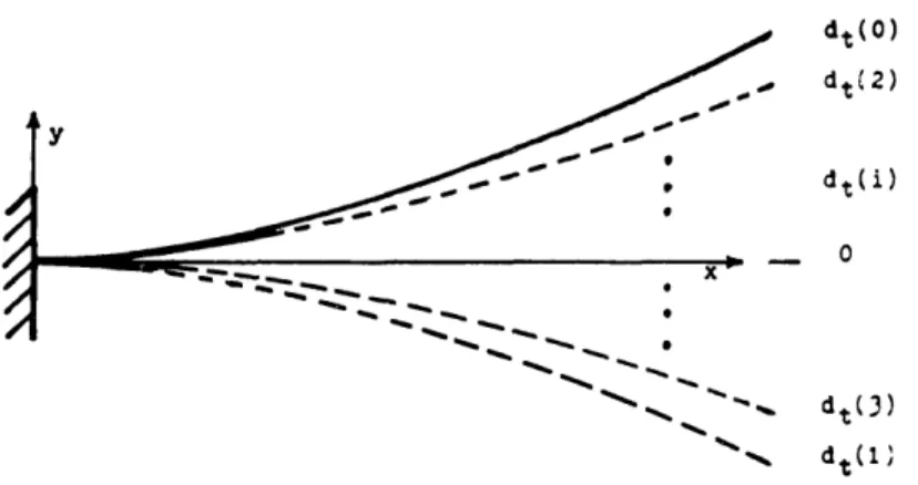
The simulation algorithm is as follows:
1. Start with the beam having some initial displacement amplitude (only one mode shape may be present) and an initial velocity of zero.
2. For each half-cycle of vibration, determine the amount of work done on the beam by the active damper and the energy dissapated by any passive damping in the system.
3. Subtract the amount of energy lost during the half-cycle from the amount of energy in the system at the beginning of the half-cycle. Use the remaining energy to determine the corresponding displacement amplitude of the banm. 4. Repeat steps 2 and 3 until the displacement amplitude reaches zero.
This algorithm assumes that the control will not significantly change the mode of vibration. The first mode of vibration and the modified Lyapunov control law were chosen to demonstrate the simulation. The tip displacement was chosen to represent the modal displacement. This simulation algorithm essentially gives the decay envelope of the vibration since the displacement amplitudes are found every half-cycle. Figure 3-4 shows the first few half-cycles of a simulation.
3.4.2 Bending strain energy as z. function of tip displacement
To implement the simulation algorithm, one must know the potential energy in the mode as a function of the modal displacement (for this case, the tip displacement). One way to find this relation is to determine the mode shape and then integrate to find the total strain energy in the composite beam as a function of the tip displacement. Since it has been assumed that the control does not change the mode shapes, this study will use the mode shapes of the uncontrolled (homogeneous) system. The procedure used to find the mode shapes is given in Appendix B.
Assuming separation of variables, the transverse motion can be separated into two parts, one that depends on space, z and another that depends on time, t, or
A II11 utv dt(2)
dt(i)
0-
-
-v_ d-
dt(X~(
3)
dt(l,Figure 3-4: Several steps of a simulation.
where ,(z) is the mode shape and f(t) is the modal amplitude. The dimensionless shape of the first mode, ,, is given by (see Appendix B)
Il(z) = cos(1.20z) - cosh(1l.20z) - 0.887( sin(1.20z) - sinh(1.20z) ) (3.24)
Next, the equation relating the modal amplitude and the tip displacement is found so that the tip displacement can be used to represent the modal displacement. The dimensionless tip displacement, dt, is given by (for the first mode)
d(t) = l,t) = -(1)u.(t)
= 0.936 · t(1) . (3.25)
Using this equation, the transverse motion of the first mode can be described by
u(z,t) = 1.07 · -(z) dt(t) (3.26)
where the tip displacement, d, represents the modal displacement.
The dimensional strain energy due to bending of the composite beam is given by (from Eqn. (A.20))
1 ' a2x d2
Lb - E l x dx (3.27)
where El is the total bending stiffness of the composite beam. To find the equivalent non-dimensional energy equation, divide this equation by El/I and substitute te dimensionless variables defined in Eqn. (3.9). This yields
1 X' a2 2
Eb 2 J a) dz . (3.28)
where E is the dimensionless bending strain energy. Substituting for the transverse motion, w, from Eqn. (3.26), using the first mode shape given in Eqn. (3.21), performing the differentiation and integration yields
:b' = g (d,)2 (3.29)
- 1.08 (d,) 2
where g is a constant (for a given mode) that expresses the dimensionless energy in the beam per unit dimensionless tip displacement squared. This is the equation relating the strain energy in the beam and tip displacement for the first mode.
3.4.3 Work done by the active damper
Another equation that is needed to implement the simulation algorithm is the work done on the beam by the active damper every half-cycle. The active damping works on the beam through the dimensionless control voltage, V, at the tip of the beam (see equations of motion, Eqns. (3.12) and (3.13)). The dimensionless work done on the system by the control voltage is given by
EC
=
f
V ·
)
at
dt
(3.30)
f,
azat
where times ti and t are the beginning and end of each half-cycle, respectively. Because the
angular velocity (and hence the linear velocity) does not changc sign during a given half-cycle (see Figure 3-4), the modified Lyapunov control law, Eqn. (3.20), calls for a constant control voltage over this time interval. This means that the integral in Eqn. (3.30) reduces to
Ec = Vmaz( 0(t) - (t;) ) (3.31)
where 0 is the tip angle, and the sign of the control voltage is determined by the modified Lyapunov control law.
Since the tip displacement is being used to represent the modal displacement, next find the relationship between the tip angle and tip displacement. The tip angle, 0, is defined by
aw
=
(3.32)
and substituting for w from Eqn. (3.26) and performing the differentiation, the equation relating tip angle to dimensionless tip displacement for the first mode is
0(t) = 1.48 dt (3.33)
= f di
where f is a constant (for a given mode) that relates the tip angle to the dimensionless tip displacement. This is the constant that is used in the modified Lyapunov control law. Substituting this equation into Eqn. (3.31) gives the work done by the control voltage in terms of the tip displacement,
E, =
Vma
zf
(
d(tl) - d(ti) )
(3.34)
or
E, = ±Vmas 1.48 ( d(tl) dr(t) ) (3.35)
for the first mode.
Using the modified Lyapunov control law (Eqn. (3.20)), the sign of the control voltage depends only on the sign of f times the linear velocity at the tip of the beam. When d(ti;) is positive, d(tl) is negative and the linear velocity during the half-cycle is negative. For this half-cycle, the control voltage will be opposite the sign of f times the linear velocity, or positive for the first mode. When d(ti) is negative, then the other parameters also switch signs. Generalizing from these relations, and using Eqn. (3.33) in Eqn. (3.31), the work done by the control voltage is
E
- V
f( d(t) - d(ti)
)(3.36)
or, for the first mode,
E = - 1.48 V
dt(t) - d(t.)
(3.37)
3.4.4 Energy dissapated by passive damping
The next step is to find the energy dissapated by passive damping per half-cycle for a given mode. The structural loss factor, eta, is defined by 1281
Edis 1
;1 = - (3.38)
Esys 2x
where EdiS is the energy dissapated during one cycle of vibration, and Esys is the total energy in the system at the beginning of the cycle. Each mode has a loss factor associated with it so the loss factor is sometimes referred to as the modal loss factor. Note that the loss factor is a dimensionless parameter and will be the same for any dynamically scaled system. For small values of Aj, the loss factor is related to the damping ratio, , of the system by 7q = 2- . The decay envelope for the vibrations of a system with very little damping can then be written as
,(t) =
(0)
exp(-)
(3.39)
where is the amplitude of the decay envelope and w is the dimensionless natural frequency. The natural frequency is found while determining the mode shape. The predicted dimensionless natural frequencies for the first four modes of the cantilever beam are listed in Table B-I. For the cantilever beam, the tip displacement at the end of the half-cycle, d(t), is given by
dit)
=dt(ti) exp(
)
(3.40)
since wt = r for a half-cycle of vibration.
From the equation for bending energy in the beam Eqn. (3.29), the energy in the beam at the end of the half-cycle is given by
Eb(t) = g d,(t)2
= g d(ti)2 exp( - ) (3.41)
= E(t) exp( -
)
where g represents the bending energy per unit tip displacement squared. The dimensionless energy dissapated during the half-cycle is the diffference, or
Ed = -(
b(t) - E(t;) )
6- (I
-exp(-wrl)
) E(t)
= g (1 - exp(-Tlr) ) d(ti)2 (3.42)
or, using the value of g for the first mode (from Eqn. (3.29), the energy dissapated per half-cycle for the first mode is
Ed- 1.08 ( - exp(-nI) ) d(ti)2 (3.43)
Note that Ed is assumed to be positive for work taken out of the system.
3.4.5 Demonstrating the simulation algorithm
The simulation algorithm described in Section 3.4.1 can be impleme.nted using the results of Sections 3.4.2, 3.4.3, and 3.4.4. The energy in the beam after the half-cycle is the energ:y that was in the beam at the beginning of the half-cycle minus the energy dissapated by passive damping (Eqn. (3.42)), and the work done by the control voltage (Eqn. (3.34)), or
Eb(t,) = Eb(t;) - Ed + E . (3.44)
Substituting the equations for the energies yields
g'
dt(t)
=g exp(-lnI)
d(t,)
Vz
f
( d(t) -
d(t)
)
.
(3.45)
This is a quadratic equation in d(t,) which can be solved using the quadratic formula. The quadratic formula gives
d
tt
Vmazf inz _ ( fd(ti))
+exp(-TI)
d(t,)*
(3.46)2*g 2g J 2 g
Using the modified Lyapunov control law, Eqn. (3.20), to determine the sign on the control voltage, and choosing the sign on the radical so that the magnitude of the tip displacement is always decreasing, one can generalize a solution to the quadratic formula as was obtained for the work done by the control voltage (see Eqn. (3.36)). The general solution is
d
1(t/)
=2
-dl2
|
(
+ exp(-n) d 2()
(3.47)
This equation is used to perform the simulation and because the absolute value of the tip displacement is found, this is essentially the decay envelope. The simulation, in terms of number of time steps, only depends on the passive damping, , and a term that includes the bending energy per tip displacement, g, the tip angle per unit tip displacement, f, and the control voltage limit, Vm,. This means that beams with the same passive damping and the same dimensionless terms (g, f, V,,,a) will have the same simulation results in terms of number of time steps (not necessarily ). It also means that beams with the same passive damping and the same value for the term Vmuf will also have the same simulation results
28
because the simulation depends on this term, not the individual values. The time interval between time steps is determined from t=/nlw because the time step spans one half-cycle of vibration.
For the parameter study, both the control voltage and the passive loss factor were varied. The symbol lp will be used to denote the passive loss factor to distinguish from the active damping. Note that since the simulation depends only on the passive damping (which is directly varied for the parameter study) and the voltage term, 2A (which is varied through V), the simulation results for any mode of a particular beam can be scaled to give the corresponding results for any mode of any other beam. The only criteria is that these two terms be the same. Since the passive loss factor is one term, the loss factor must be the same for both beams. The control voltage term would be scaled by choosing the control voltage limit so the voltage term would be the same for both beams. For instance, the simulation results for a beam with Vma=g=f=10 would be the same as for a beam with Vz=g=l and f=10, for a given passive loss factor. The dimensionless time would then be scaled by the ratio of the natural frequencies or eigenvalues for the given mode of the beams. The dimensional results would then be found as usual by using the definitions of the dimensionless variables given in Eqn. (3.9).
There are several cases when certain parameters would not have to be rescaled to find the results for one mode of a beam from those of another. Since the dimensionless frequency, w, depends only on the eigenvalue of the mode (Fee Appendix B), when two beams have the same eigenvalue their dimensionless time scales, t, will also be the same. This means the results from the dimensionless simulation of one mode of a beam can be scaled to correspond to those of a different beam (a mode that has the same eigenvalue! without rescaling the time axis (i.e., only change the control voltage). This does not mean that the
mode shapes are also the same (i.e., the dimensionless tip masses and tip inertias are different, but the eigenvalues happen to be the same). If the dimensionless tip masses and tip inertias are the same, then the eigenvalues and the mode shapes will both be the same for the two beams (see Appendix B). Since the dimensionless terms g and f depend only on the eigenvalue and mode shape, the beams will have the same simulation results (in terms of the number of time steps) for a given control voltage, V,,z, and passive loss factor, p. This means the dimensionless simulation results for a mode of one beam are the same as those for any other beam with the same dimensionless tip mass and tip inertia.
For the first mode of the scaled cantilever beam, the simulation equation is
d(t) = -0.687. Vmz (3.48)
+ /(0.687 Vma)2 - 1.37 Vmas dt(t) + exp(-,n) d2(ti)
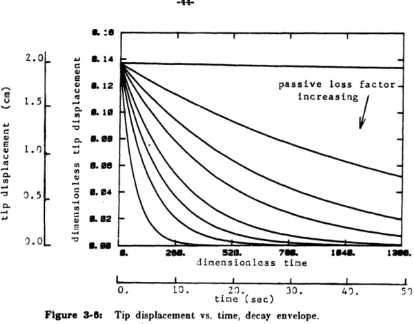
The results of two simulation cases are shown in Figure 3-5 and are labeled with both dimensionless and dimensional axes. The dimensional axes are for the scaled cantilever beam. The initial conditions were chosen .as d(0)= 0.146 (2 cm tip displacement for the scaled beam). Figure 3-5a shows a case with a minimum control voltage limit, Vmaz= 4x10- (a dimensional voltage of 1 V for the scaled beam) and a passive loss factor of -p= 0.010 . Note that the measured torque constant, c, was used to non-dimensionalize the control voltage. (See Section 4.2.1.) The decay envelope for this case is nearly exponential because the control voltage is so low and the passive damping is dissapating most of the energy in the beam. However, the active control does have a noticeable effect at very small displacements. A true exponential decay envelope would approach zero amplitude, but never reach it. In this case, the beam does reach zero near t= 800 (t=30 sec. for the scaled beam). Figure 3-5 b shows a case with a moderate control voltage, Vz- 4x10⁻⁴ (100 V for the scaled beam) and no passive damping, p=0.000 . Notice that the decay envelope is linear, not exponential. This indicates nonlinear damping and is the result of the nonlinear modified Lyapunov control law doing all the damping.
In comparing the two simulation cases, one should note several points. First, the slope of the passively damped case is initially much higher than the actively damped slope, indicating the passive damping is taking more energy out of the beam than the active damping. However, the slope of the passively damped case changes because of the exponential decay envelope and soon becomes less than the actively damped slope (which is constant), now indicating the active damping is more effective. This is because the passive
dimensionless
tip displacement1.14
1.12
I. 1S . O1. 14
3.-0
(a). Free decay of first V =-4x1O-. B. 253. 523. V0I'". 1349. dimensionless time mode simulation. ip = 0.010 dimensionless tip displacement
0.14
1. 12 M. s B. so M. 0 B. M3.13 B. 283. 523. 780. dimensionless tilme 1040. 1300.(b). Free decay of first mode simulation. n = 0 000 V -4x10 -4 .
Figure 35: Typical simulation results for free decay of first mode.
![Figure 2-2: Flexible test structure at the Ch:arles Stark Draper Laboratory [1].](https://thumb-eu.123doks.com/thumbv2/123doknet/14751898.580583/18.918.193.762.158.636/figure-flexible-test-structure-arles-stark-draper-laboratory.webp)