Dynamic Graph CNN for Learning on Point Clouds

Dynamic Graph CNN for Learning on Point Clouds

The MIT Faculty has made this article openly available.

Please share

how this access benefits you. Your story matters.

Citation

Wang, Yue et al. "Dynamic Graph CNN for Learning on Point

Clouds." ACM Transactions on Graphics 38, 5 (October 2019): 146 ©

2019 The Author(s)

As Published

http://dx.doi.org/10.1145/3326362

Publisher

Association for Computing Machinery (ACM)

Version

Author's final manuscript

Citable link

https://hdl.handle.net/1721.1/126819

Terms of Use

Creative Commons Attribution-Noncommercial-Share Alike

YUE WANG,

YONGBIN SUN,

ZIWEI LIU,

SANJAY E. SARMA,

MICHAEL M. BRONSTEIN,

JUSTIN M. SOLOMON,

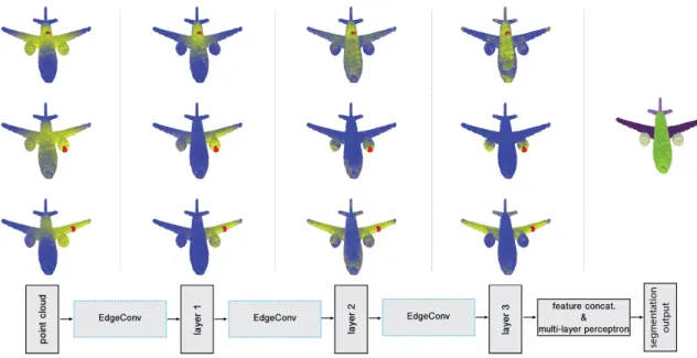
Fig. 1. Point cloud segmentation using the proposed neural network. Bottom: schematic neural network architecture. Top: Structure of the feature spaces produced at different layers of the network, visualized as the distance from the red point to all the rest of the points (shown left-to-right are the input and layers 1-3; rightmost figure shows the resulting segmentation). Observe how the feature space structure in deeper layers captures semantically similar structures such as wings, fuselage, or turbines, despite a large distance between them in the original input space.

Point clouds provide a flexible geometric representation suitable for count-less applications in computer graphics; they also comprise the raw output of most 3D data acquisition devices. While hand-designed features on point clouds have long been proposed in graphics and vision, however, the recent overwhelming success of convolutional neural networks (CNNs) for image analysis suggests the value of adapting insight from CNN to the point cloud world. Point clouds inherently lack topological information so designing

Authors’ addresses: Yue Wang, Massachusetts Institute of Technology, yuewang@ csail.mit.edu; Yongbin Sun, Massachusetts Institute of Technology, yb_sun@mit.edu; Ziwei Liu, UC Berkeley / ICSI, zwliu@icsi.berkeley.edu; Sanjay E. Sarma, Massachusetts Institute of Technology, sesarma@mit.edu; Michael M. Bronstein, Imperial College London / USI Lugano, m.bronstein@imperial.ac.uk; Justin M. Solomon, Massachusetts Institute of Technology, jsolomon@mit.edu.

Permission to make digital or hard copies of all or part of this work for personal or classroom use is granted without fee provided that copies are not made or distributed for profit or commercial advantage and that copies bear this notice and the full citation on the first page. Copyrights for components of this work owned by others than the author(s) must be honored. Abstracting with credit is permitted. To copy otherwise, or republish, to post on servers or to redistribute to lists, requires prior specific permission and /or a fee. Request permissions from permissions@acm.org.

© 2019 Copyright held by the owner/author(s). Publication rights licensed to ACM. 0730-0301/2019/1-ART1 $15.00

https://doi.org/10.1145/3326362

a model to recover topology can enrich the representation power of point clouds. To this end, we propose a new neural network module dubbed Edge-Conv suitable for CNN-based high-level tasks on point clouds including classification and segmentation. EdgeConv acts on graphs dynamically com-puted in each layer of the network. It is differentiable and can be plugged into existing architectures. Compared to existing modules operating in extrinsic space or treating each point independently, EdgeConv has several appealing properties: It incorporates local neighborhood information; it can be stacked applied to learn global shape properties; and in multi-layer systems affinity in feature space captures semantic characteristics over potentially long dis-tances in the original embedding. We show the performance of our model on standard benchmarks including ModelNet40, ShapeNetPart, and S3DIS.

CCS Concepts: •Computing methodologies → Neural networks; Point-based models;Shape analysis;

Additional Key Words and Phrases: point cloud, classification, segmentation

ACM Reference Format:

Yue Wang, Yongbin Sun, Ziwei Liu, Sanjay E. Sarma, Michael M. Bronstein, and Justin M. Solomon. 2019. Dynamic Graph CNN for Learning on Point Clouds.ACM Trans. Graph. 1, 1, Article 1 (January 2019), 13 pages. https: //doi.org/10.1145/3326362

1 INTRODUCTION

Point clouds, or scattered collections of points in 2D or 3D, are arguably the simplest shape representation; they also comprise the output of 3D sensing technology including LiDAR scanners and stereo reconstruction. With the advent of fast 3D point cloud acquisition, recent pipelines for graphics and vision often process point clouds directly, bypassing expensive mesh reconstruction or denoising due to efficiency considerations or instability of these techniques in the presence of noise. A few of the many recent applications of point cloud processing and analysis include indoor navigation [Zhu et al. 2017], self-driving vehicles [Liang et al. 2018; Qi et al. 2017a; Wang et al. 2018b], robotics [Rusu et al. 2008b], and shape synthesis and modeling [Golovinskiy et al. 2009; Guerrero et al. 2018].

These modern applications demandhigh-level processing of point clouds. Rather than identifying salient geometric features like cor-ners and edges, recent algorithms search for semantic cues and affordances. These features do not fit cleanly into the frameworks of computational or differential geometry and typically require learning-based approaches that derive relevant information through statistical analysis of labeled or unlabeled datasets.

In this paper, we primarily consider point cloud classification and segmentation, two model tasks in point cloud processing. Tra-ditional methods for solving these problems employ handcrafted features to capture geometric properties of point clouds [Lu et al. 2014; Rusu et al. 2009, 2008a]. More recently, the success of deep neural networks for image processing has motivated a data-driven approach to learning features on point clouds. Deep point cloud pro-cessing and analysis methods are developing rapidly and outperform traditional approaches in various tasks [Chang et al. 2015].

Adaptation of deep learning to point cloud data, however, is far from straightforward. Most critically, standard deep neural network models require input data with regular structure, while point clouds are fundamentally irregular: Point positions are continuously dis-tributed in the space, and any permutation of their ordering does not change the spatial distribution. One common approach to pro-cess point cloud data using deep learning models is to first convert raw point cloud data into a volumetric representation, namely a 3D grid [Maturana and Scherer 2015; Wu et al. 2015]. This approach, however, usually introduces quantization artifacts and excessive memory usage, making it difficult to go to capture high-resolution or fine-grained features.

State-of-the-art deep neural networks are designed specifically to handle the irregularity of point clouds, directly manipulating raw point cloud data rather than passing to an intermediate regular repre-sentation. This approach was pioneered byPointNet [Qi et al. 2017b], which achieves permutation invariance of points by operating on each point independently and subsequently applying a symmetric function to accumulate features. Various extensions of PointNet consider neighborhoods of points rather than acting on each inde-pendently [Qi et al. 2017c; Shen et al. 2017]; these allow the network to exploit local features, improving upon performance of the basic model. These techniques largely treat points independently at local

scale to maintain permutation invariance. This independence, how-ever, neglects the geometric relationships among points, presenting a fundamental limitation that cannot capture local features.

To address these drawbacks, we propose a novel simple operation, called EdgeConv, which captures local geometric structure while maintaining permutation invariance. Instead of generating point features directly from their embeddings, EdgeConv generatesedge features that describe the relationships between a point and its neighbors. EdgeConv is designed to be invariant to the ordering of neighbors, and thus is permutation invariant. Because EdgeConv explicitly constructs a local graph and learns the embeddings for the edges, the model is capable of grouping points both in Euclidean space and in semantic space.

EdgeConv is easy to implement and integrate into existing deep learning models to improve their performance. In our experiments, we integrate EdgeConv into the basic version ofPointNet without using any feature transformation. We show the resulting network achieves state-of-the-art performance on several datasets, most no-tablyModelNet40 and S3DIS for classification and segmentation.

Key Contributions. We summarize the key contributions of our work as follows:

• We present a novel operation for learning from point clouds, EdgeConv, to better capture local geometric features of point clouds while still maintaining permutation invariance.

• We show the model can learn to semantically group points by dynamically updating a graph of relationships from layer to layer. • We demonstrate that EdgeConv can be integrated into multiple

existing pipelines for point cloud processing.

• We present extensive analysis and testing of EdgeConv and show that it achieves state-of-the-art performance on benchmark datasets. • We release our code to facilitate reproducibility and future

re-search.1

2 RELATED WORK

Hand-Crafted Features. Various tasks in geometric data process-ing and analysis—includprocess-ing segmentation, classification, and matchprocess-ing— require some notion of local similarity between shapes. Traditionally, this similarity is established by constructing feature descriptors that capture local geometric structure. Countless papers in computer vi-sion and graphics propose local feature descriptors for point clouds suitable for different problems and data structures. A comprehensive overview of hand-designed point features is out of the scope of this paper, but we refer the reader to [Biasotti et al. 2016; Guo et al. 2014; Van Kaick et al. 2011] for discussion.

Broadly speaking, one can distinguish betweenextrinsic and in-trinsic descriptors. Exin-trinsic descriptors usually are derived from the coordinates of the shape in 3D space and includes classical methods like shape context [Belongie et al. 2001], spin images [Johnson and Hebert 1999], integral features [Manay et al. 2006], distance-based descriptors [Ling and Jacobs 2007], point feature histograms [Rusu et al. 2009, 2008a], and normal histograms [Tombari et al. 2011], to name a few. Intrinsic descriptors treat the 3D shape as a manifold whose metric structure is discretized as a mesh or graph; quantities

1

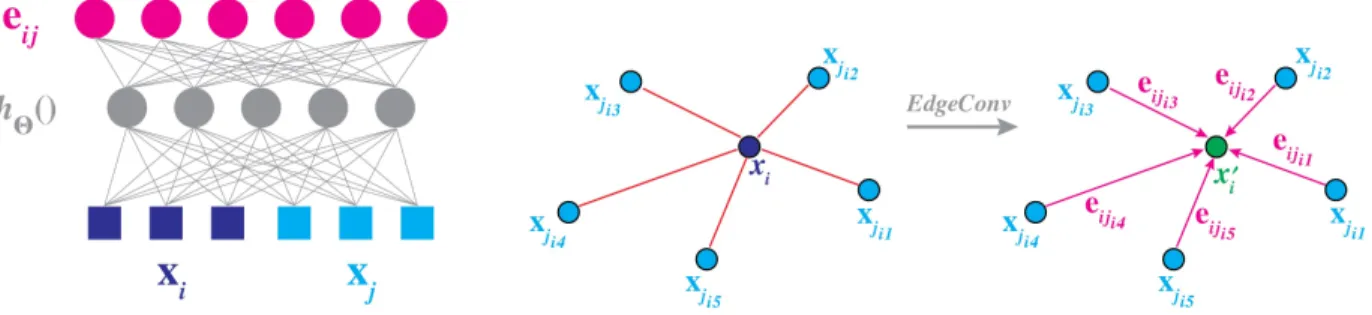
Fig. 2. Left: Computing an edge feature, ei j(top), from a point pair, xiand xj(bottom). In this example, hΘ()is instantiated using a fully connected layer, and the learnable parameters are its associated weights. Right: The EdgeConv operation. The output of EdgeConv is calculated by aggregating the edge features associated with all the edges emanating from each connected vertex.

expressed in terms of the metric are invariant to isometric defor-mation. Representatives of this class include spectral descriptors such as global point signatures [Rustamov 2007], the heat and wave kernel signatures [Aubry et al. 2011; Sun et al. 2009], and variants [Bronstein and Kokkinos 2010]. Most recently, several approaches wrap machine learning schemes around standard descriptors [Guo et al. 2014; Shah et al. 2013].

Deep learning on geometry. Following the breakthrough results of convolutional neural networks (CNNs) in vision [Krizhevsky et al. 2012; LeCun et al. 1989], there has been strong interest to adapt such methods to geometric data. Unlike images, geometry usually does not have an underlying grid, requiring new building blocks replacing convolution and pooling or adaptation to a grid structure. As a simple way to overcome this issue, view-based [Su et al. 2015; Wei et al. 2016] and volumetric representations [Klokov and Lempit-sky 2017; Maturana and Scherer 2015; Tatarchenko et al. 2017; Wu et al. 2015]—or their combination [Qi et al. 2016]—“place” geometric data onto a grid. More recently, PointNet [Qi et al. 2017b,c] exempli-fies a broad class of deep learning architectures on non-Euclidean data (graphs and manifolds) termedgeometric deep learning [Bron-stein et al. 2017]. These date back to early methods to construct neural networks on graphs [Scarselli et al. 2009], recently improved with gated recurrent units [Li et al. 2016] and neural message pass-ing [Gilmer et al. 2017]. Bruna et al. [2013] and Henaff et al. [2015] generalized convolution to graphs via the Laplacian eigenvectors [Shuman et al. 2013]. Computational drawbacks of this foundational approach were alleviated in follow-up works using polynomial [Def-ferrard et al. 2016; Kipf and Welling 2017; Monti et al. 2017b, 2018], or rational [Levie et al. 2017] spectral filters that avoid Laplacian eigendecomposition and guarantee localization. An alternative def-inition of non-Euclidean convolution employs spatial rather than spectral filters. TheGeodesic CNN (GCNN) is a deep CNN on meshes generalizing the notion of patches using local intrinsic parameteriza-tion [Masci et al. 2015]. Its key advantage over spectral approaches is better generalization as well as a simple way of constructing directional filters. Follow-up work proposed different local chart-ing techniques uschart-ing anisotropic diffusion [Boscaini et al. 2016] or Gaussian mixture models [Monti et al. 2017a; Veličković et al. 2017]. In [Halimi et al. 2018; Litany et al. 2017b], a differentiable functional map [Ovsjanikov et al. 2012] layer was incorporated into

a geometric deep neural network, allowing to do intrinsic structured prediction of correspondence between nonrigid shapes.

The last class of geometric deep learning approaches attempts to pull back a convolution operation by embedding the shape into a domain with shift-invariant structure such as the sphere [Sinha et al. 2016], torus [Maron et al. 2017], plane [Ezuz et al. 2017], sparse network lattice [Su et al. 2018], or spline [Fey et al. 2018].

Finally, we should mentiongeometric generative models, which attempt to generalize models such as autoencoders, variational au-toencoders (VAE) [Kingma and Welling 2013], and generative adver-sarial networks (GAN) [Goodfellow et al. 2014] to the non-Euclidean setting. One of the fundamental differences between these two set-tings is the lack of canonical order between the input and the output vertices, thus requiring an input-output correspondence problem to be solved. In 3D mesh generation, it is commonly assumed that the mesh is given and its vertices are canonically ordered; the gen-eration problem thus amounts only to determining the embedding of the mesh vertices. Kostrikov et al. [2017] proposed SurfaceNets based on the extrinsic Dirac operator for this task. Litany et al. [2017a] introduced the intrinsic VAE for meshes and applied it to shape completion; a similar architecture was used by Ranjan et al. [2018] for 3D face synthesis. For point clouds, multiple generative architectures have been proposed [Fan et al. 2017; Li et al. 2018b; Yang et al. 2018].

3 OUR APPROACH

We propose an approach inspired by PointNet and convolution operations. Instead of working on individual points like PointNet, however, we exploit local geometric structures by constructing a local neighborhood graph and applying convolution-like operations on the edges connecting neighboring pairs of points, in the spirit of graph neural networks. We show in the following that such an operation, dubbededge convolution (EdgeConv), has properties lying between translation-invariance and non-locality.

Unlike graph CNNs, our graph is not fixed but rather is dynam-ically updated after each layer of the network. That is, the set of k-nearest neighbors of a point changes from layer to layer of the network and is computed from the sequence of embeddings. Prox-imity in feature space differs from proxProx-imity in the input, leading to nonlocal diffusion of information throughout the point cloud. As

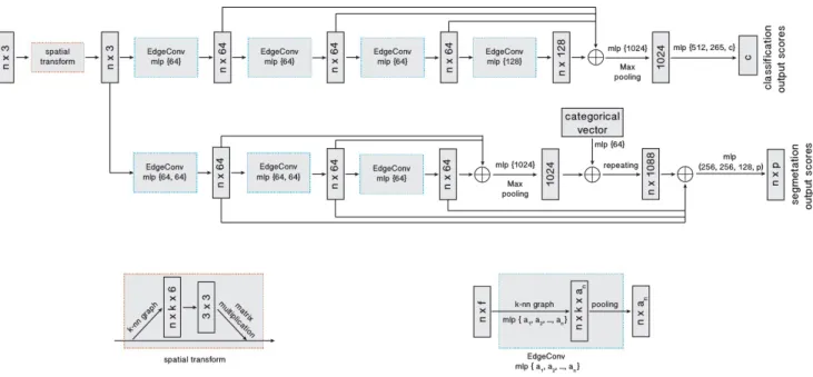
Fig. 3. Model architectures: The model architectures used for classification (top branch) and segmentation (bottom branch). The classification model takes as input n points, calculates an edge feature set of size k for each point at an EdgeConv layer, and aggregates features within each set to compute EdgeConv responses for corresponding points. The output features of the last EdgeConv layer are aggregated globally to form an 1D global descriptor, which is used to generate classification scores for c classes. The segmentation model extends the classification model by concatenating the 1D global descriptor and all the EdgeConv outputs (serving as local descriptors) for each point. It outputs per-point classification scores for p semantic labels. ⊕: concatenation. Point cloud transform block:The point cloud transform block is designed to align an input point set to a canonical space by applying an estimated 3 × 3 matrix. To estimate the 3 × 3 matrix, a tensor concatenating the coordinates of each point and the coordinate differences between its k neighboring points is used. EdgeConv block:The EdgeConv block takes as input a tensor of shape n × f , computes edge features for each point by applying a multi-layer perceptron (mlp) with the number of layer neurons defined as {a1, a2, ..., a_n}, and generates a tensor of shape n × a_nafter pooling among neighboring edge features.

a connection to existing work, Non-local Neural Networks [Wang et al. 2018a] explored similar ideas in the video recognition field, and follow-up work by Xie et al. [2018] proposed using non-local blocks to denoise feature maps to defend against adversarial attacks.

3.1 Edge Convolution

Consider anF -dimensional point cloud with n points, denoted by X= {x1, . . . , xn} ⊆ RF. In the simplest setting ofF = 3, each point

contains 3D coordinatesx_i = (x_i,y_i, z_i); it is also possible to include additional coordinates representing color, surface normal, and so on. In a deep neural network architecture, each subsequent layer operates on the output of the previous layer, so more generally the dimensionF represents the feature dimensionality of a given layer. We compute a directed graphG= (V, E) representing local point cloud structure, whereV = {1, . . . ,n} and E ⊆ V × V are the vertices and edges, respectively. In the simplest case, we construct G as thek-nearest neighbor (k-NN) graph of X in RF. The graph includes self-loop, meaning each node also points to itself. We define edge features asei j = hΘ(xi, xj), wherehΘ: RF × RF → RF

′

is a nonlinear function with a set of learnable parametersΘ.

Finally, we define the EdgeConv operation by applying a channel-wise symmetric aggregation operation□ (e.g.,Íor max) on the edge features associated with all the edges emanating from each

vertex. The output of EdgeConv at thei-th vertex is thus given by x_i′=

□

j:(i, j)∈ E

h_Θ(xi, xj). (1)

Making analogy to convolution along images, we regardx_i as the central pixel and{x_j : (i, j) ∈ E} as a patch around it (see Fig-ure 2). Overall, given anF -dimensional point cloud with n points, EdgeConv produces anF′-dimensional point cloud with the same number of points.

Choice ofh and □. The choice of the edge function and the ag-gregation operation has a crucial influence on the properties of EdgeConv. For example, whenx1, . . . , x_n represent image pixels

on a regular grid and the graphG has connectivity representing patches of fixed size around each pixel, the choiceθ_m· x_j as the edge function and sum as the aggregation operation yields standard convolution: x′ im= Õ j:(i, j)∈ E θm· xj, (2)

Here,Θ = (θ1, . . . , θ_M) encodes the weights ofM different filters.

Eachθ_m has the same dimensionality asx, and · denotes the Eu-clidean inner product.

A second choice ofh is

encoding only global shape information oblivious of the local neigh-borhood structure. This type of operation is used in PointNet, which can thus be regarded as a special case of EdgeConv.

A third choice ofh adopted by Atzmon et al. [2018] is

h_Θ(xi, xj)= hΘ(xj) (4) and x′ im = Õ j ∈V (hθ (xj))д(u(xi, xj)), (5)

whereд is a Gaussian kernel and u computes pairwise distance in Euclidean space.

A fourth option is

h_Θ(xi, xj)= h_Θ(xj− xi). (6) This encodes only local information, treating the shape as a collec-tion of small patches and losing global structure.

Finally, a fifth option that we adopt in this paper is an asymmetric edge function

h_Θ(xi, xj)= ¯hΘ(xi, xj− xi). (7) This explicitly combines global shape structure, captured by the coordinates of the patch centersx_i, with local neighborhood infor-mation, captured byx_j−x_i. In particular, we can define our operator by notating

e′

i jm= ReLU(θm· (xj− xi)+ ϕm· xi), (8) which can be implemented as a shared MLP, and taking

x′ im = max j:(i, j)∈ Ee ′ i jm, (9) whereΘ = (θ₁, . . . , θ_M, ϕ 1, . . . , ϕM)

3.2 Dynamic graph update

Our experiments suggest that it is beneficial torecompute the graph using nearest neighbors in the feature space produced by each layer. This is a crucial distinction of our method from graph CNNs working on a fixed input graph. Such a dynamic graph update is the reason for the name of our architecture, theDynamic Graph CNN (DGCNN). With dynamic graph updates, the receptive field is as large as the diameter of the point cloud, while being sparse.

At each layer we have a different graphG(l )= (V(l ), E(l )), where thel-th layer edges are of the form (i, j_{i 1}), . . . , (i, j_ik

l) such that

x(l )_j

i 1, . . . , x

(l )

j_{i kl} are thekl points closest tox(l )

i . Put differently, our

architecture learnshow to construct the graph G used in each layer rather than taking it as a fixed constant constructed before the network is evaluated. In our implementation, we compute a pairwise distance matrix in feature space and then take the closestk points for each single point.

3.3 Properties

Permutation Invariance. Consider the output of a layer x_i′= max

j:(i, j)∈ EhΘ(xi, xj)

(10) and a permutation operatorπ. The output of the layer x′

iis invariant

to permutation of the inputx_jbecause max is a symmetric function (other symmetric functions also apply). The global max pooling operator to aggregate point features is also permutation-invariant.

Translation Invariance. Our operator has a “partial” translation invariance property, in that our choice of edge functions (7) explicitly exposes the part of the function that can be translation-dependent and optionally can be disabled. Consider a translation applied tox_j andx_i; we can show that part of the edge feature is preserved when shifting byT . In particular, for the translated point cloud we have

e′

i jm= θm· (xj+ T − (xi+ T )) + ϕm· (xi+ T )

= θm· (xj− xi)+ ϕm· (xi+ T ).

If we only considerx_j− x_iby takingϕ

m= 0, then the operator

is fully invariant to translation. In this case, however, the model re-duces to recognizing an object based on an unordered set of patches, ignoring the positions and orientations of patches. With bothx_j− x_i andx_i as input, the model takes account into the local geometry of patches while keeping global shape information.

3.4 Comparison to existing methods

DGCNN is related to two classes of approaches, PointNet and graph CNNs, which we show to be particular settings of our method. We summarize different methods in Table 1.

PointNet is a special case of our method withk = 1, yielding a graph with an empty edge setE = ∅. The edge function used in PointNet ish_Θ(x_i, x_j)= h_Θ(x_i), which considers global but not local geometry. PointNet++ tries to account for local structure by ap-plying PointNet in a local manner. In our parlance, PointNet++ first constructs the graph according to the Euclidean distances between the points, and in each layer applies a graph coarsening operation. For each layer, some points are selected using farthest point sam-pling (FPS); only the selected points are preserved while others are directly discarded after this layer. In this way, the graph becomes smaller after the operation applied on each layer. In contrast to DGCNN, PointNet++ computes pairwise distances using point in-put coordinates, and hence their graphs are fixed during training. The edge function used by PointNet++ ish_Θ(x_i, x_j)= h_Θ(x_j), and the aggregation operation is also a max.

Among graph CNNs, MoNet [Monti et al. 2017a], ECC [Simonovsky and Komodakis 2017], Graph Attention Networks [Veličković et al. 2017], and the concurrent work [Atzmon et al. 2018] are the most related approaches. Their common denominator is a notion of a local patch on a graph, in which a convolution-type operation can be defined.2

Specifically, Monti et al. [2017a] use the graph structure to com-pute a local “pseudo-coordinate system”u in which the neighbor-hood vertices are represented; the convolution is then defined as an M-component Gaussian mixture

x′ im =

Õ

j:(i, j)∈ E

θm· (xj⊙дwn(u(xi, xj))), (11)

whereд is a Gaussian kernel, ⊙ is the elementwise (Hadamard) prod-uct,{w₁, . . . , w_N} encode the learnable parameters of the Gaussians (mean and covariance), and{θ1, . . . , θ_M} are the learnable filter

co-efficients. (11) is an instance of our general operation (1), with a

2

[Simonovsky and Komodakis 2017; Veličković et al. 2017] can be considered instances of [Monti et al. 2017a], with the difference that the weights are constructed employing features from adjacent nodes instead of graph structure; [Atzmon et al. 2018] is also similar except that the weighting function is hand-designed.

Aggregation

Edge Function

Learnable parameters

PointNet [Qi et al. 2017b]

—

h

(x

, x

)

= h

(x

)

Θ

PointNet++ [Qi et al. 2017c]

max

h

(x

, x

)

= h

(x

)

Θ

MoNet [Monti et al. 2017a]

Í

h

m,wn

(x

, x

)

= θ

· (x

⊙

д

(u(x

, x

)))

w

, θ

PCNN [Atzmon et al. 2018]

Í

h

m

(x

, x

)

= (θ

· x

)д(u(x

, x

))

θ

Table 1. Comparison to existing methods. The per-point weight wi in [Atzmon et al. 2018] effectively is computed in the first layer and could be carried

onward as an extra feature; we omit this for simplicity.

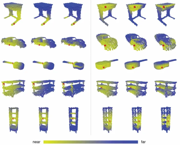
Fig. 4. Structure of the feature spaces produced at different stages of our shape classification neural network architecture, visualized as the distance between the red point to the rest of the points. For each set, Left: Euclidean distance in the input R3

space; Middle: Distance after the point cloud transform stage, amounting to a global transformation of the shape; Right: Distance in the feature space of the last layer. Observe how in the feature space of deeper layers semantically similar structures such as shelves of a bookshelf or legs of a table are brought close together, although they are distant in the original space.

particular edge function

h_θm,wn(xi, xj)= θm· (xj⊙дwn(u(xi, xj)))

and□ =Í. Again, their graph structure is fixed, andu is constructed based on the degrees of nodes.

[Atzmon et al. 2018] can be seen as a special case of [Monti et al. 2017a] withд as predefined Gaussian functions. Removing learnable parameters(w1, . . . , w_N) and constructing a dense graph from point

clouds, we have x′ im= Õ j:j ∈V (θm· xj)д(u(xi, xj)), (12)

whereu is the pairwise distance between x_i andx_j in Euclidean space.

While MoNet and other graph CNNs assume a given fixed graph on which convolution-like operations are applied, to our knowledge our method is the first for which the graph changes from layer to layer and even on the same input during training when learnable parameters are updated. This way, our model not only learns how to extract local geometric features, but also how to group points in a point cloud. Figure 4 shows the distance in different feature spaces, exemplifying that the distances in deeper layers carry semantic information over long distances in the original embedding.

4 EVALUATION

In this section, we evaluate the models constructed using EdgeConv for different tasks: classification, part segmentation, and semantic segmentation. We also visualize experimental results to illustrate key differences from previous work.

4.1 Classification

Data. We evaluate our model on the ModelNet40 [Wu et al. 2015] classification task, consisting in predicting the category of a pre-viously unseen shape. The dataset contains 12,311 meshed CAD models from 40 categories. 9,843 models are used for training and 2,468 models are for testing. We follow verbatim the experimental settings of Qi et al. [2017b]. For each model, 1,024 points are uni-formly sampled from the mesh faces; the point cloud is rescaled to fit into the unit sphere. Only the(x,y, z) coordinates of the sam-pled points are used, and the original meshes are discarded. During the training procedure, we augment the data by randomly scaling objects and perturbing the object and point locations.

Architecture. The network architecture used for the classification task is shown in Figure 3 (top branch without spatial transformer network). We use four EdgeConv layers to extract geometric fea-tures. The four EdgeConv layers use three shared fully-connected layers(64, 64, 128, 256). We recompute the graph based on the fea-tures of each EdgeConv layer and use the new graph for next layer. The numberk of nearest neighbors is 20 for all EdgeConv layers (for the last row in Table 2,k is 40). Shortcut connections are included to extract multi-scale features and one shared fully-connected layer (1024) to aggregate multi-scale features, where we concatenate fea-tures from previous layers to get a 64+64+128+256=512 dimensional point cloud. Then, a global max/sum pooling is used to get the point cloud global feature, after which two fully-connected layers (512, 256) are used to transform the global feature. Dropout with

keep probability of 0.5 is used in the last two fully-connected layers. All layers include LeakyReLU and batch normalization. The number k was chosen using a validation set. We split the training data to 80% for training and 20% for validation to search the bestk. After k is chosen, we retrain the model on the whole training data and evaluate the model on the testing data. Other hyperparameters were chosen in a similar ways.

Training. We use SGD with learning rate 0.1, and we reduce the learning rate until 0.001 using cosine annealing [Loshchilov and Hutter 2017]. The momentum for batch normalization is 0.9, and we do not use batch normalization decay. The batch size is 32 and the momentum is 0.9.

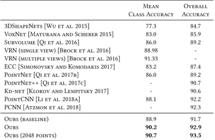
Results. Table 2 shows the results for the classification task. Our model achieves the best results on this dataset. Our baseline using a fixed graph determined by proximity in the input point cloud is 1.0% better than PointNet++. An advanced version including dynamical graph recomputation achieves the best results on this dataset. All the experiments are performed with point clouds that contain 1024 points except last row. We further test out model with 2048 points. Thek used for 2048 points is 40 to maintain the same density. Note that PCNN [Atzmon et al. 2018] uses additional augmentation techniques like randomly sampling 1024 points out of 1200 points during both training and testing.

Mean Overall Class Accuracy Accuracy 3DShapeNets [Wu et al. 2015] 77.3 84.7 VoxNet [Maturana and Scherer 2015] 83.0 85.9 Subvolume [Qi et al. 2016] 86.0 89.2 VRN (single view) [Brock et al. 2016] 88.98 -VRN (multiple views) [Brock et al. 2016] 91.33 -ECC [Simonovsky and Komodakis 2017] 83.2 87.4 PointNet [Qi et al. 2017b] 86.0 89.2 PointNet++ [Qi et al. 2017c] - 90.7 Kd-net [Klokov and Lempitsky 2017] - 90.6 PointCNN [Li et al. 2018a] 88.1 92.2 PCNN [Atzmon et al. 2018] - 92.3 Ours (baseline) 88.9 91.7

Ours 90.2 92.9

Ours (2048 points) 90.7 93.5 Table 2. Classification results on ModelNet40.

4.2 Model Complexity

We use the ModelNet40 [Wu et al. 2015] classification experiment to compare the complexity of our model to previous state-of-the-art. Table 3 shows that our model achieves the best tradeoff between the model complexity (number of parameters), computational complex-ity (measured as forward pass time), and the resulting classification accuracy.

Our baseline model using the fixedk-NN graph outperforms the previous state-of-the-art PointNet++ by 1.0% accuracy, at the same time being 7 times faster. A more advanced version of our model including a dynamically-updated graph computation outperforms PointNet++, PCNN by 2.2% and 0.6% respectively, while being much

Model size(MB) Time(ms) Accuracy(%)

PointNet (Baseline) [Qi et al. 2017b] 9.4 6.8 87.1 PointNet [Qi et al. 2017b] 40 16.6 89.2 PointNet++ [Qi et al. 2017c] 12 163.2 90.7 PCNN [Atzmon et al. 2018] 94 117.0 92.3

Ours (Baseline) 11 19.7 91.7

Ours 21 27.2 92.9

Table 3. Complexity, forward time, and accuracy of different models

more efficient. The number of points in each experiment is also 1024 in this section.

4.3 More Experiments on ModelNet40

We also experiment with various settings of our model on the Mod-elNet40 [Wu et al. 2015] dataset. In particular, we analyze the effec-tiveness of the different distance metrics, explicit usage ofx_i− x_j, and more points.

Table 4 shows the results. “Centralization” denotes using con-catenation ofx_iandx_i − x_jas the edge features rather than con-catenatingx_i andx_j. “Dynamic graph recomputation” denotes we reconstruct the graph rather than using a fixed graph. Explicitly centralizing each patch by using the concatenation ofx_iandx_i− x_j leads to about 0.5% improvement for overall accuracy. By dynami-cally updating graph, there is about 0.7% improvement, and Figure 4 also suggests that the model can extract semantically meanigful features. Using more points further improves the overall accuracy by 0.6%.

We also experiment with different numbersk of nearest neighbors as shown in Table 5. For all experiments, the number of points is still 1024. While we do not exhaustively experiment with all possiblek, we find with large k that the performance degenerates. This confirms our hypothesis that for certain density, with large k the Euclidean distance fails to approximate geodesic distance, destroying the geometry of each patch.

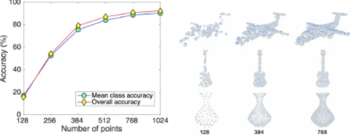
We further evaluate the robustness of our model (trained on 1,024 points withk = 20) to point cloud density. We simulate the environment that random input points drops out during testing. Figure 5 shows that even half of points is dropped, the model still achieves reasonable results. With fewer than 512 points, however, performance degenerates dramatically.

CENT DYN MPOINTS Mean Class Accuracy(%) Overall Accuracy(%)

88.9 91.7

x 89.3 92.2

x x 90.2 92.9

x x x 90.7 93.5

Table 4. Effectiveness of different components. CENT denotes centraliza-tion, DYN denotes dynamical graph recomputacentraliza-tion, and MPOINTS denotes experiments with 2048 points

.

Fig. 5. Left: Results of our model tested with random input dropout. The model is trained with number of points being 1024 and k being 20. Right: Point clouds with different number of points. The numbers of points are shown below the bottom row.

Number of nearest neighbors (k) Mean Overall Class Accuracy(%) Accuracy(%)

5 88.0 90.5

10 88.9 91.4

20 90.2 92.9

40 89.4 92.4

Table 5. Results of our model with different numbers of nearest neighbors.

4.4 Part Segmentation

Data. We extend our EdgeConv model architectures for part seg-mentation task on ShapeNet part dataset [Yi et al. 2016]. For this task, each point from a point cloud set is classified into one of a few predefined part category labels. The dataset contains 16,881 3D shapes from 16 object categories, annotated with 50 parts in total. 2,048 points are sampled from each training shape, and most sampled point sets are labeled with less than six parts. We follow the official train/validation/test split scheme as Chang et al. [2015] in our experiment.

Architecture. The network architecture is illustrated in Figure 3 (bottom branch). After a spatial transformer network, three Edge-Conv layers are used. A shared fully-connected layer(1024) aggre-gates information from the previous layers. Shortcut connections are used to include all the EdgeConv outputs as local feature de-scriptors. At last, three shared fully-connected layers(256, 256, 128) are used to transform the pointwise features. Batch-norm, dropout, and ReLU are included in the similar fashion to our classification network.

Training. The same training setting as in our classification task is adopted. A distributed training scheme is further implemented on two NVIDIA TITAN X GP Us to maintain the training batch size. Results. We use Intersection-over-Union (IoU) on points to eval-uate our model and compare with other benchmarks. We follow the same evaluation scheme as PointNet: The IoU of a shape is computed by averaging the IoUs of different parts occurring in that shape, and the IoU of a category is obtained by averaging the IoUs of all the shapes belonging to that category. The mean IoU (mIoU) is finally calculated by averaging the IoUs of all the testing shapes. We

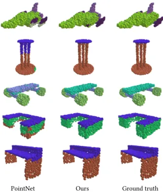
Fig. 6. Our part segmentation testing results for tables, chairs and lamps.

compare our results with PointNet [Qi et al. 2017b], PointNet++ [Qi et al. 2017c], Kd-Net [Klokov and Lempitsky 2017], LocalFeatureNet [Shen et al. 2017], PCNN [Atzmon et al. 2018], and PointCNN [Li et al. 2018a]. The evaluation results are shown in Table 6. We also visually compare the results of our model and PointNet in Figure 7. More examples are shown in Figure 6.

Intra-cloud distances. We next explore the relationships between different point clouds captured using our features. As shown in Figure 8, we take one red point from a source point cloud and compute its distance in feature space to points in other point clouds from the same category. An interesting finding is that although points are from different sources, they are close to each other if they are from semantically similar parts. We evaluate on the features after the third layer of our segmentation model for this experiment. Segmentation on partial data. Our model is robust to partial data. We simulate the environment that part of the shape is dropped from one of six sides (top, bottom, right, left, front and back) with different percentages. The results are shown in Figure 9. On the left,

PointNet Ours Ground truth

Fig. 7. Compare part segmentation results. For each set, from left to right: PointNet, ours and ground truth.

the mean IoU versus “keep ratio” is shown. On the right, the results for an airplane model are visualized.

4.5 Indoor Scene Segmentation

Data. We evaluate our model on Stanford Large-Scale 3D Indoor Spaces Dataset (S3DIS) [Armeni et al. 2016] for a semantic scene segmentation task. This dataset includes 3D scan point clouds for 6 indoor areas including 272 rooms in total. Each point belongs to one of 13 semantic categories—e.g. board, bookcase, chair, ceiling, and beam—plus clutter. We follow the same setting as Qi et al. [2017b], where each room is split into blocks with area 1m × 1m, and each point is represented as a 9D vector (XYZ, RGB, and normalized spatial coordinates). 4,096 points are sampled for each block during training process, and all points are used for testing. We also use the same 6-fold cross validation over the 6 areas, and the average evaluation results are reported.

The model used for this task is similar to part segmentation model, except that a probability distribution over semantic object classes is generated for each input point and no categorical vector is used here. We compare our model with both PointNet [Qi et al. 2017b] and PointNet baseline, where additional point features (local point den-sity, local curvature and normal) are used to construct handcrafted features and then fed to an MLP classifier. We further compare our work with [Engelmann et al. 2017] and PointCNN [Li et al. 2018a]. Engelmann et al. [2017] present network architectures to enlarge the receptive field over the 3D scene. Two different approaches are proposed in their work: MS+CU for multi-scale block features with consolidation units; G+RCU for the grid-blocks with recurrent

mean areo bag cap car chair ear guitar knife lamp laptop motor mug pistol rocket skate table . phone board # shapes 2690 76 55 898 3758 69 787 392 1547 451 202 184 283 66 152 5271 PointNet 83.7 83.4 78.7 82.5 74.9 89.6 73.0 91.5 85.9 80.8 95.3 65.2 93.0 81.2 57.9 72.8 80.6 PointNet++ 85.1 82.4 79.0 87.7 77.3 90.8 71.8 91.0 85.9 83.7 95.3 71.6 94.1 81.3 58.7 76.4 82.6 Kd-Net 82.3 80.1 74.6 74.3 70.3 88.6 73.5 90.2 87.2 81.0 94.9 57.4 86.7 78.1 51.8 69.9 80.3 LocalFeatureNet 84.3 86.1 73.0 54.9 77.4 88.8 55.0 90.6 86.5 75.2 96.1 57.3 91.7 83.1 53.9 72.5 83.8 PCNN 85.1 82.4 80.1 85.5 79.5 90.8 73.2 91.3 86.0 85.0 95.7 73.2 94.8 83.3 51.0 75.0 81.8 PointCNN 86.1 84.1 86.45 86.0 80.8 90.6 79.7 92.3 88.4 85.3 96.1 77.2 95.3 84.2 64.2 80.0 83.0 Ours 85.2 84.0 83.4 86.7 77.8 90.6 74.7 91.2 87.5 82.8 95.7 66.3 94.9 81.1 63.5 74.5 82.6

Table 6. Part segmentation results on ShapeNet part dataset. Metric is mIoU(%) on points.

Source points Other point clouds from the same category

Fig. 8. Visualize the Euclidean distance (yellow: near, blue: far) between source points (red points in the left column) and multiple point clouds from the same category in the feature space after the third EdgeConv layer. Notice source points not only capture semantically similar structures in the point clouds that they belong to, but also capture semantically similar structures in other point clouds from the same category.

consolidation Units. We report evaluation results in Table 7, and visually compare the results of PointNet and our model in Figure 10.

Fig. 9. Left: The mean IoU (%) improves when the ratio of kept points in-creases. Points are dropped from one of six sides (top, bottom, left, right, front and back) randomly during evaluation process. Right: Part segmentation results on partial data. Points on each row are dropped from the same side. The keep ratio is shown below the bottom row. Note that the segmentation results of turbines are improved when more points are included.

Mean overall IoU accuracy PointNet (baseline) [Qi et al. 2017b] 20.1 53.2 PointNet [Qi et al. 2017b] 47.6 78.5 MS + CU(2) [Engelmann et al. 2017] 47.8 79.2 G + RCU [Engelmann et al. 2017] 49.7 81.1 PointCNN [Li et al. 2018a] 65.39

-Ours 56.1 84.1

Table 7. 3D semantic segmentation results on S3DIS. MS+CU for multi-scale block features with consolidation units; G+RCU for the grid-blocks with recurrent consolidation Units.

5 DISCUSSION

In this work we propose a new operator for learning on point cloud and show its performance on various tasks. Our model suggests that local geometric features are important to 3D recognition tasks, even after introducing machinery from deep learning.

While our architectures easily can be incorporated as-is into existing pipelines for point cloud-based graphics, learning, and vision, our experiments also indicate several avenues for future research and extension. Some details of our implementation could be revised and/or re-engineered to improve efficiency or scalability, e.g. incorporating fast data structures rather than computing pairwise

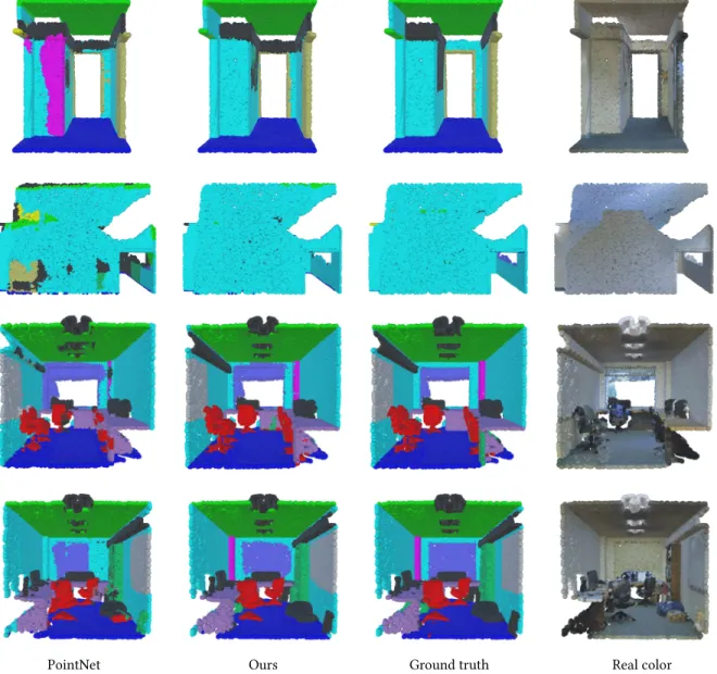
PointNet Ours Ground truth Real color

Fig. 10. Semantic segmentation results. From left to right: PointNet, ours, ground truth and point cloud with original color. Notice our model outputs smoother segmentation results, for example, wall (cyan) in top two rows, chairs (red) and columns (magenta) in bottom two rows.

distances to evaluatek-nearest neighbors queries. We also could consider higher-order relationships between larger tuples of points, rather than considering them pairwise. Another possible extension is to design a non-shared transformer network that works on each local patch differently, adding flexibility to our model.

Our experiments suggest that intrinsic features can be equally valuable if not more valuable than point coordinates; developing a practical and theoretically-justified framework for balancing intrin-sic and extrinintrin-sic considerations in a learning pipeline will require insight from theory and practice in geometry processing. Given this, we will consider applications of our techniques to more abstract point clouds coming from applications like document retrieval and image processing rather than 3D geometry; beyond broadening

the applicability of our technique, these experiments will provide insight into the role of geometry in abstract data processing.

ACKNOWLEDGMENTS

The authors acknowledge the generous support of Army Research Office grant W911NF-12-R-0011, of Air Force Office of Scientific Research award FA9550-19-1-0319, of National Science Foundation grant IIS-1838071, of ERC Consolidator grant No. 724228 (LEMAN), from an Amazon Research Award, from the MIT-IBM Watson AI Laboratory, from the Toyota-CSAIL Joint Research Center, from the Skoltech-MIT Next Generation Program, and from Google Faculty

Research Award. Any opinions, findings, and conclusions or recom-mendations expressed in this material are those of the authors and do not necessarily reflect the views of these organizations.

REFERENCES

Iro Armeni, Ozan Sener, Amir R. Zamir, Helen Jiang, Ioannis Brilakis, Martin Fischer, and Silvio Savarese. 2016. 3D Semantic Parsing of Large-Scale Indoor Spaces. In Proc. CVPR.

Matan Atzmon, Haggai Maron, and Yaron Lipman. 2018. Point Convolutional Neural Networks by Extension Operators._{ACM Trans. Graph. 37, 4, Article 71 (July 2018),} 12 pages. https://doi.org/10.1145/3197517.3201301

Mathieu Aubry, Ulrich Schlickewei, and Daniel Cremers. 2011. The Wave Kernel Signature: A Quantum Mechanical Approach to Shape Analysis. In_{Proc. ICCV} Workshops.

Serge Belongie, Jitendra Malik, and Jan Puzicha. 2001. Shape Context: A New Descriptor for Shape Matching and Object Recognition. InProc. NIPS.

Silvia Biasotti, Andrea Cerri, A Bronstein, and M Bronstein. 2016. Recent Trends, Ap-plications, and Perspectives in 3D Shape Similarity assessment.Computer Graphics Forum 35, 6 (2016), 87–119.

Davide Boscaini, Jonathan Masci, Emanuele Rodolà, and Michael Bronstein. 2016. Learning Shape Correspondence with Anisotropic Convolutional Neural Networks. InProc. NIPS.

Andrew Brock, Theodore Lim, James Millar Ritchie, and Nicholas J. Weston. 2016. Generative and Discriminative Voxel Modeling with Convolutional Neural Networks. InProc. NIPS.

Michael M Bronstein, Joan Bruna, Yann LeCun, Arthur Szlam, and Pierre Vandergheynst. 2017. Geometric Deep Learning: Going beyond Euclidean Data.IEEE Signal Process-ing Magazine 34, 4 (2017), 18–42.

Michael M Bronstein and Iasonas Kokkinos. 2010. Scale-invariant Heat Kernel Signa-tures for Non-rigid Shape Recognition. In_{Proc. CVPR.}

Joan Bruna, Wojciech Zaremba, Arthur Szlam, and Yann LeCun. 2013. Spectral Networks and Locally Connected Networks on Graphs._{arXiv:1312.6203 (2013).}

Angel X Chang, Thomas Funkhouser, Leonidas Guibas, Pat Hanrahan, Qixing Huang, Zimo Li, Silvio Savarese, Manolis Savva, Shuran Song, Hao Su, et al. 2015. Shapenet: An Information-rich 3D Model Repository._{arXiv:1512.03012 (2015).}

Michaël Defferrard, Xavier Bresson, and Pierre Vandergheynst. 2016. Convolutional Neural Networks on Graphs with Fast Localized Spectral Filtering. In_{Proc. NIPS.} Francis Engelmann, Theodora Kontogianni, Alexander Hermans, and Bastian Leibe.

2017. Exploring Spatial Context for 3D Semantic Segmentation of Point Clouds. In Proc. CVPR.

Danielle Ezuz, Justin Solomon, Vladimir G Kim, and Mirela Ben-Chen. 2017. GWCNN: A Metric Alignment Layer for Deep Shape Analysis.Computer Graphics Forum 36, 5 (2017), 49–57.

Haoqiang Fan, Hao Su, and Leonidas J Guibas. 2017. A Point Set Generation Network for 3D Object Reconstruction from a Single Image.. InProc. CVPR.

Matthias Fey, Jan Eric Lenssen, Frank Weichert, and Heinrich Müller. 2018. SplineCNN: Fast Geometric Deep Learning with Continuous B-Spline Kernels. InIEEE Conference on Computer Vision and Pattern Recognition (CVPR).

Justin Gilmer, Samuel S Schoenholz, Patrick F Riley, Oriol Vinyals, and George E Dahl. 2017. Neural Message Passing for Quantum Chemistry._{arXiv:1704.01212 (2017).} Aleksey Golovinskiy, Vladimir G. Kim, and Thomas Funkhouser. 2009. Shape-based

Recognition of 3D Point Clouds in Urban Environments. In_{Proc. ICCV.} Ian Goodfellow, Jean Pouget-Abadie, Mehdi Mirza, Bing Xu, David Warde-Farley, Sherjil

Ozair, Aaron Courville, and Yoshua Bengio. 2014. Generative Adversarial Nets. In Proc. NIPS.

Paul Guerrero, Yanir Kleiman, Maks Ovsjanikov, and Niloy J. Mitra. 2018.PCPNet: Learning Local Shape Properties from Raw Point Clouds._{Computer Graphics Forum} 37, 2 (2018), 75–85. https://doi.org/10.1111/cgf.13343

Yulan Guo, Mohammed Bennamoun, Ferdous Sohel, Min Lu, and Jianwei Wan. 2014. 3D Object Recognition in Cluttered Scenes with Local Surface Features: a Survey. Trans. PAMI 36, 11 (2014), 2270–2287.

Oshri Halimi, Or Litany, Emanuele Rodolà, Alex Bronstein, and Ron Kimmel. 2018. Self-supervised Learning of Dense Shape Correspondence.arXiv:1812.02415 (2018). M. Henaff, J. Bruna, and Y. LeCun. 2015. Deep Convolutional Networks on

Graph-structured Data.arXiv:1506.05163 (2015).

Andrew E. Johnson and Martial Hebert. 1999. Using Spin Images for Efficient Object Recognition in Cluttered 3D Scenes.Trans. PAMI 21, 5 (1999), 433–449. DiederikPKingmaand MaxWelling.2013. Auto-encodingVariationalBayes.

arXiv:1312.6114 (2013).

Thomas N Kipf and Max Welling. 2017.Semi-supervised Classification with Graph Convolutional Networks. (2017).

Roman Klokov and Victor Lempitsky. 2017. Escape from Cells: Deep Kd-Networks for The Recognition of 3D Point Cloud Models. (2017).

Ilya Kostrikov, Zhongshi Jiang, Daniele Panozzo, Denis Zorin, and Joan Bruna. 2017. Surface Networks. In_{Proc. CVPR.}

Alex Krizhevsky, Ilya Sutskever, and Geoffrey E Hinton. 2012. Imagenet Classification with Deep Convolutional Neural Networks. In_{Proc. NIPS.}

Yann LeCun, Bernhard Boser, John S Denker, Donnie Henderson, Richard E Howard, Wayne Hubbard, and Lawrence D Jackel. 1989. Backpropagation Applied to Hand-written ZIP Code Recognition._{Neural computation 1, 4 (1989), 541–551.} Ron Levie, Federico Monti, Xavier Bresson, and Michael M Bronstein. 2017. CayleyNets:

Graph Convolutional Neural Networks with Complex Rational Spectral Filters. arXiv:1705.07664 (2017).

Chun-Liang Li, Manzil Zaheer, Yang Zhang, Barnabas Poczos, and Ruslan Salakhutdinov. 2018b. Point Cloud GAN.arXiv:1810.05795 (2018).

Yangyan Li, Rui Bu, Mingchao Sun, Wei Wu, Xinhan Di, and Baoquan Chen. 2018a. PointCNN: Convolution On X-Transformed Points.InAdvances in Neural Infor-mation Processing Systems 31, S. Bengio, H. Wallach, H. Larochelle, K. Grauman, N. Cesa-Bianchi, and R. Garnett (Eds.). Curran Associates, Inc., 820–830. http: //papers.nips.cc/paper/7362- pointcnn- convolution- on- x- transformed- points.pdf Yujia Li, Daniel Tarlow, Marc Brockschmidt, and Richard Zemel. 2016. Gated graph

Sequence Neural Networks. InProc. ICLR.

Ming Liang, Bin Yang, Shenlong Wang, and Raquel Urtasun. 2018. Deep Continuous Fu-sion for Multi-Sensor 3D Object Detection. In_{The European Conference on Computer} Vision (ECCV).

Haibin Ling and David W Jacobs. 2007. Shape Classification using the Inner-distance. Trans. PAMI 29, 2 (2007), 286–299.

Or Litany, Alex Bronstein, Michael Bronstein, and Ameesh Makadia. 2017a. Deformable Shape Completion with Graph Convolutional Autoencoders. _{arXiv:1712.00268} (2017).

Or Litany, Tal Remez, Emanuele Rodolà, Alex M Bronstein, and Michael M Bronstein. 2017b. Deep Functional Maps: Structured Prediction for Dense Shape Correspon-dence. In_{Proc. ICCV.}

I. Loshchilov and F. Hutter. 2017. SGDR: Stochastic Gradient Descent with Warm Restarts. InInternational Conference on Learning Representations (ICLR) 2017 Confer-ence Track.

Min Lu, Yulan Guo, Jun Zhang, Yanxin Ma, and Yinjie Lei. 2014. Recognizing Objects in 3D Point Clouds with Multi-scale Local Features.Sensors 14, 12 (2014), 24156–24173. Siddharth Manay, Daniel Cremers, Byung-Woo Hong, Anthony J Yezzi, and Stefano Soatto. 2006.Integral Invariants for Shape Matching.Trans. PAMI 28, 10 (2006), 1602–1618.

Haggai Maron, Meirav Galun, Noam Aigerman, Miri Trope, Nadav Dym, Ersin Yumer, Vladimir G Kim, and Yaron Lipman. 2017. Convolutional Neural Networks on Surfaces via Seamless Toric Covers. InProc. SIGGRAPH.

Jonathan Masci, Davide Boscaini, Michael Bronstein, and Pierre Vandergheynst. 2015. Geodesic Convolutional Neural Networks on Riemannian Manifolds. In_{Proc. 3dRR.} Daniel Maturana and Sebastian Scherer. 2015.Voxnet: A 3D Convolutional Neural

Network for Real-time Object Recognition. In_{Proc. IROS.}

Federico Monti, Davide Boscaini, Jonathan Masci, Emanuele Rodolà, Jan Svoboda, and Michael M Bronstein. 2017a. Geometric Deep Learning on Graphs and Manifolds using Mixture Model CNNs. In_{Proc. CVPR.}

F. Monti, M. M. Bronstein, and X. Bresson. 2017b. Geometric Matrix Completion with Recurrent Multi-graph Neural Networks. In_{Proc. NIPS.}

Federico Monti, Karl Otness, and Michael M Bronstein. 2018. MotifNet: A Motif-based Graph Convolutional Network for Directed Graphs._{arXiv:1802.01572 (2018).} Maks Ovsjanikov, Mirela Ben-Chen, Justin Solomon, Adrian Butscher, and Leonidas

Guibas. 2012. Functional Maps: A Flexible Representation of Maps between Shapes. TOG 31, 4 (2012), 30.

Charles R Qi, Wei Liu, Chenxia Wu, Hao Su, and Leonidas J Guibas. 2017a. Frustum PointNets for 3D Object Detection from RGB-D Data.arXiv:1711.08488 (2017). Charles R. Qi, Hao Su, Kaichun Mo, and Leonidas J. Guibas. 2017b.PointNet: Deep

Learning on Point Sets for 3D Classification and Segmentation. InProc. CVPR. Charles R Qi, Hao Su, Matthias Nießner, Angela Dai, Mengyuan Yan, and Leonidas J

Guibas. 2016.Volumetric and Multi-view CNNs for Object Classification on 3D Data. InProc. CVPR.

Charles R. Qi, Li Yi, Hao Su, and Leonidas J. Guibas. 2017c. PointNet++: Deep Hierar-chical Feature Learning on Point Sets in a Metric Space. InProc. NIPS.

Anurag Ranjan, Timo Bolkart, Soubhik Sanyal, and Michael J Black. 2018. Generating 3D faces using Convolutional Mesh Autoencoders._{arXiv:1807.10267 (2018).} Raif M Rustamov. 2007. Laplace-Beltrami Eigenfunctions for Deformation Invariant

Shape Representation. In_{Proc. SGP.}

Radu Bogdan Rusu, Nico Blodow, and Michael Beetz. 2009. Fast Point Feature His-tograms (FPFH) for 3D Registration. In_{Proc. ICRA.}

Radu Bogdan Rusu, Nico Blodow, Zoltan Csaba Marton, and Michael Beetz. 2008a. Aligning Point Cloud Views using Persistent Feature Histograms. In_{Proc. IROS.} Radu Bogdan Rusu, Zoltan Csaba Marton, Nico Blodow, Mihai Dolha, and Michael Beetz.

2008b. Towards 3D Point Cloud Based Object Maps for Household Environments. Robotics and Autonomous Systems Journal 56, 11 (30 November 2008), 927–941. Franco Scarselli, Marco Gori, Ah Chung Tsoi, Markus Hagenbuchner, and Gabriele

Monfardini. 2009. The Graph Neural Network Model.IEEE Tran. Neural Networks 20, 1 (2009), 61–80.

Syed Afaq Ali Shah, Mohammed Bennamoun, Farid Boussaid, and Amar A El-Sallam. 2013. 3D-Div: A novel Local Surface Descriptor for Feature Matching and Pairwise Range Image Registration. In_{Proc. ICIP.}

Yiru Shen, Chen Feng, Yaoqing Yang, and Dong Tian. 2017. Neighbors Do Help: Deeply Exploiting Local Structures of Point Clouds._{arXiv:1712.06760 (2017).}

David I Shuman, Sunil K Narang, Pascal Frossard, Antonio Ortega, and Pierre Van-dergheynst. 2013. The Emerging Field of Signal Processing on Graphs: Extending High-dimensional Data Analysis to Networks and Other Irregular Domains.IEEE Signal Processing Magazine 30, 3 (2013), 83–98.

Martin Simonovsky and Nikos Komodakis. 2017. Dynamic Edge-Conditioned Filters in Convolutional Neural Networks on Graphs. InProc. CVPR.

Ayan Sinha, Jing Bai, and Karthik Ramani. 2016.Deep Learning 3D shape Surfaces using Geometry Images. InProc. ECCV.

Hang Su, Varun Jampani, Deqing Sun, Subhransu Maji, Evangelos Kalogerakis, Ming-Hsuan Yang, and Jan Kautz. 2018. SPLATNet: Sparse Lattice Networks for Point Cloud Processing. InProceedings of the IEEE Conference on Computer Vision and Pattern Recognition. 2530–2539.

Hang Su, Subhransu Maji, Evangelos Kalogerakis, and Erik Learned-Miller. 2015. Multi-view Convolutional Neural Networks for 3D Shape Recognition. In_{Proc. CVPR.} Jian Sun, Maks Ovsjanikov, and Leonidas Guibas. 2009. A Concise and Provably

Informative Multi-scale Signature based on Heat Diffusion. _{Computer Graphics} Forum 28, 5 (2009), 1383–1392.

Maxim Tatarchenko, Alexey Dosovitskiy, and Thomas Brox. 2017. Octree Generating Networks: Efficient Convolutional Architectures for High-resolution 3D Outputs. In_{Proc. ICCV.}

Federico Tombari, Samuele Salti, and Luigi Di Stefano. 2011. A Combined Texture-shape Descriptor for Enhanced 3D Feature Matching. In_{Proc. ICIP.}

Oliver Van Kaick, Hao Zhang, Ghassan Hamarneh, and Daniel Cohen-Or. 2011. A Survey on Shape Correspondence.Computer Graphics Forum 30, 6 (2011), 1681–1707. Petar Veličković, Guillem Cucurull, Arantxa Casanova, Adriana Romero, Pietro Liò,

and Yoshua Bengio. 2017. Graph Attention Networks.arXiv:1710.10903 (2017). Shenlong Wang, Simon Suo, Wei-Chiu Ma, Andrei Pokrovsky, and Raquel Urtasun.

2018b. Deep Parametric Continuous Convolutional Neural Networks. InThe IEEE Conference on Computer Vision and Pattern Recognition (CVPR).

Xiaolong Wang, Ross Girshick, Abhinav Gupta, and Kaiming He. 2018a.Non-local Neural Networks.CVPR (2018).

Lingyu Wei, Qixing Huang, Duygu Ceylan, Etienne Vouga, and Hao Li. 2016. Dense Human Body Correspondences using Convolutional Networks. InProc. CVPR. Zhirong Wu, Shuran Song, Aditya Khosla, Fisher Yu, Linguang Zhang, Xiaoou Tang,

and Jianxiong Xiao. 2015.3D Shapenets: A Deep Representation for Volumetric Shapes. In_{Proc. CVPR.}

CihangXie,YuxinWu,LaurensvanderMaaten,AlanYuille,andKaimingHe. 2018. Feature Denoising for Improving Adversarial Robustness. _{arXiv preprint} arXiv:1812.03411 (2018).

Yaoqing Yang, Chen Feng, Yiru Shen, and Dong Tian. 2018. FoldingNet: Point Cloud Auto-Encoder via Deep Grid Deformation. In_{Proc. CVPR.}

Li Yi, Vladimir G Kim, Duygu Ceylan, I Shen, Mengyan Yan, Hao Su, ARCewu Lu, Qixing Huang, Alla Sheffer, Leonidas Guibas, et al. 2016. A Scalable Active Framework for Region Annotation in 3D Shape Collections._{TOG 35, 6 (2016), 210.}

Yuke Zhu, Roozbeh Mottaghi, Eric Kolve, Joseph J. Lim, Abhinav Gupta, Li Fei-Fei, and Ali Farhadi. 2017. Target-driven Visual Navigation in Indoor Scenes using Deep Reinforcement learning. InProc. ICRA.