Exact nonlinear analytic Vlasov-Maxwell tangential equilibria with arbitrary density and temperature profiles

HAL Id: hal-00001083

https://hal.archives-ouvertes.fr/hal-00001083

HAL is a multi-disciplinary open access

archive for the deposit and dissemination of sci-entific research documents, whether they are pub-lished or not. The documents may come from

L’archive ouverte pluridisciplinaire HAL, est destinée au dépôt et à la diffusion de documents scientifiques de niveau recherche, publiés ou non, émanant des établissements d’enseignement et de

Exact nonlinear analytic Vlasov-Maxwell tangential

equilibria with arbitrary density and temperature

profiles

Fabrice Mottez

To cite this version:

Fabrice Mottez. Exact nonlinear analytic Vlasov-Maxwell tangential equilibria with arbitrary density and temperature profiles. Physics of Fluids, American Institute of Physics, 2003, 10, Phys. Plasmas, 10, pp. 2501-2508. �hal-00001083�

ccsd-00001083 (version 1) : 28 Jan 2004

Exact nonlinear analytic Vlasov-Maxwell

tangential equilibria with arbitrary density

and temperature profiles

F. Mottez,

Centre d’´etude des Environnements Terrestre et Plan´etaires (CETP),

10-12 Av. de l’Europe, 78140 V´elizy, France.

(e-mail: fabrice.mottez@cetp.ipsl.fr)

January 28, 2004

Abstract

The tangential layers are characterized by a bulk plasma velocity and a magnetic field that are perpendicular to the gradient direction. They have been extensively described in the frame of the Magneto-Hydro-Dynamic (MHD) theory. But the MHD theory does not look inside the transition region if the transition has a size of a few ion gy-roradii. A series of kinetic tangential equilibria, valid for a collisionless plasma is presented. These equilibria are exact analytical solutions of the Maxwell-Vlasov equations. The particle distribution functions are sums of an infinite number of elementary functions parametrized by a vector potential. Examples of equilibria relevant to space plasmas are shown. A model for the deep and sharp density depletions observed in the auroral zone of the Earth is proposed. Tangential equilibria are also relevant for the study of planetary environments and of remote astrophysical plasmas.

c

Copyright (2003) American Institute of Physics. This article may be downloaded for personal use only. Any other use requires prior permission of the author and the American Institute of Physics. The following article appeared in Phys. Plasmas, Vol 10, 7, pp2501,2508, and may be found at http://link.aip.org/link/?php/10/2501.

I. INTRODUCTION

The swedish Viking spacecraft orbiting in the auroral region of the magne-tosphere discovered deep plasma density depletions [1]. Their size along the magnetic field direction reach thousands of kilometers. They can be con-sidered as channels parallel to the magnetic field. These observation were confirmed by measurements onboard the Fast Auroral SnapshoT explorer (FAST) spacecraft [2]. The data showed a lot of plasma activity in and around these regions, particularly plasma acceleration (at the origin of the polar auroras) [3], electromagnetic radiation [4] and a high level of electro-static turbulence. Most of the studies focused on the acceleration [5], [6] and the nature of the turbulence [7], [8] [9]. But surprisingly, little work has been devoted to the structure of these plasma cavities. Some theoretical works have been devoted to their origin, but none has tackled the question : are auroral plasma cavities in equilibrium, or do they vanish a soon as the cause of their formation disapears ?

The aim of the work presented in this paper is to construct a kinetic model of the auroral plasma cavities. But as a very general solution to this problem is found, the field of applications appears much wider. I present here a family of equilibrium solutions that can be used in many domains of the physics of plasmas. They will be named as tangential equilibria because, as in the MHD tangential discontinuities, the magnetic field and the bulk velocities are tangential to the plane (y, z) of invariance.

Previous works on tangential equilibria [10], [11] have shown the existence of simple isothermal solutions that can be computed analytically. Other works, mainly focused on the study of the Earth magnetopause [12], have shown solutions that satisfy a larger class of constraints, but they cannot be constructed analytically.

Most of these equilibria a based, for each species, on distribution functions that are products of an exponential function of the total energy and of p2

z, by an arbitrary g function of py, f = (αzα 2 ⊥ π3 ) 1/2 [exp (−αzv2z − α⊥v2⊥)] g(mvy+ qAy(x)), (1)

where αz = m/2Tz = 1/v2tz, α⊥ = m/2T⊥ = 1/v2_t⊥, are the reciprocals of the

squared thermal velocities ; vz = pz/m and v⊥2 = v_x2+ v_y2. If g(∞) ∼ 1, then

Krall and Rosenbluth, [13] have derived a solution of the linearized ki-netic equations, by setting g(py) as a linear function. They used this simple

solution for the study of gradient instabilities.

Many authors (reviewed by Roth et al. [12]), who studied tangential discontinuities, considered solutions with g functions that involve error func-tions. Most of these studies where developed for the study of the equilibrium of the Earth magnetopause. They include an electric field Ex and no charge

neutrality. There is no analytical solution. The differential equations on Ex

and A are solved through a numerical integration.

Channell [11] considered solutions with no electric field. He showed that

Jy = T⊥

dn dAy

. (2)

A more general formula will be shown in Sec. II.

In the same paper, Channell studied a few examples of solutions with simple but nonlinear g functions. In particular, he showed that there exists a solution with g(py) = exp (−ηp2y), where η is a constant number.

Harris [10] built an equilibrium model of a current sheet. His model was widely used later for the study of the tearing mode instability. The Harris current sheet equilibrium corresponds to the case g(py) = exp (νpy).

All the solutions mentionned above are based on elementary g functions. They do not let the possibility of setting a priori a density profile, as in the more simple MHD and bi-fluid models. We can build a distribution function that is the sum of such elementary distribution functions and assert that each elementary part of the distribution corresponds to a family of trapped particles.

Because of the nonlinearity of the equations, the density and temperature profiles associated to a sum of families of trapped particles are not simple combinations of the profiles associated to single elementary particle distri-butions. Nethertheless, using a numerical equation solver, Roth et al. [12] added up to four elementary distributions functions (all of them were built with error functions). Differential equations were solved numerically.

I show in this paper how to combine an infinite number of elementary solutions and build a plasma that is made of a continuum of famillies of trapped particles. The plasma equilibria presented in this paper are com-puted analytically. They do not have the high degree of generality of those shown in Roth et al. [12], (because I impose a null electric field), but they

are more general than those of Harris [10], and Channell [11]. In particular, the plasma does not have to be isothermal.

The equations of the kinetic model are developed and solved in Sec. II. The properties of the solutions and some particular cases are briefly analysed in Sec. III. An equilibrium model for the deep non isothermal density deple-tions of the Earth auroral zone is presented. The last section is a discussion about other applications and further developments.

II. FORMULATION OF THE

MAXWELL-VLASOV MODEL

We consider a monodimensional equilibrium : ∂t = 0 and ∇ = (dx, 0, 0).

We choose the z direction along the constant direction of the magnetic field ~

B = (0, 0, Bz(x)), (∇ · B = 0 is therefore ensured). The magnetic field

derives from a vector potential ~A(x) = (0, Ay(x), 0) such that Bz = dxAy.

This vector potential satisfies the Lorentz gauge (that is ∇·~A = 0 in the stationary case). The x direction is called the normal direction, the y, z plane is the tangential plane.

In a monodimensional equilibrium, the particles are confined between two points where vx = 0. In the case of a null electric field, the size ∆x of this

area is

∆x = 2v⊥/ < ω_c > (3)

where < ωc >= (q/m∆x)

Rx₂

x1 Bz(x). Absolutely no restriction on the

varia-tions of Bx is made.

As we look for a monodimensional equilibrium, the total energy E =

mv2

2 + qΦ of any particle and the generalized momentum py = mvy+ qAy and

pz = mvz are the invariants of the motion. Any distribution function of the

form f = f (E, py, pz) is a solution of the Valsov equation. All the kinetic

solutions studied in this paper will be of that form. The other character imposed on the solutions is a null electric field, and therefore no charge separation.

The basic idea is to decompose linearly the g function (already men-tionned in Eq. 1 ) over a set of elementary distribution functions that corre-spond to an analytical equilibrium solution. As will be shown in this section, if the sum is parametrized by a parameter a that correspond to shifts of the

elementary distribution functions in the space of the potential vectors (and not in the space of the configurations), there is an analytical solution.

For instance, we can show that a continuous linear combination of Chan-nell and Harris-like g distribution functions given by

g(py) = n0+

Z a2

a1

da ng(a) exp [−η(a)(

py m − q ma) 2_{+ ν(a)(}py m − q ma)], (4) leads to an equilibrium that can be computed analytically.

The functions ng(a), η(a) > 0, and ν(a) are defined almost arbitrarily

and n0 is a constant scalar. Each of these three functions provide a degree

of freedom and it is possible, as in MHD and bi-fluid models, to control the plasma density profile. But the distribution of the particles depends on the energy through an exponential factor that does not give any freedom to set the temperature profile. Therefore, instead of using 1 and 4, let us set :

f = Z a2 a1 da (αz(a)α 2 ⊥(a) π ) 1/2_e(−αz(a)(vz−uz)2−α⊥(a)v2⊥)(n 0+ ga(py)) (5) and ga(py) = ng(a)e −_η(a)(py m− q ma) 2_+ν(a)(py m− q ma). (6)

With these distribution functions, a control of the plasma density profile (through ng(a)) and of the temperature profile of each species (through αz(a)

and α⊥(a)) is possible. The parameter a is homogeneous to a vector potential.

In order not to overload the equations, we do not express systematically the dependance of the parameters on a and x hereafter.

To solve the charge neutrality equation (ni = ne) and the Amp`ere

equa-tion

− d

2

dx2Ay = µ0Jy, (7)

we need to compute the contribution of each species s to the charge density,

ns = Z a2 a1 da (α⊥ π ) 1/2Z _dv y exp (−α⊥v_y2)g(mv_y+ qA_y(x)). (8)

and to the current density,

Jys = Z a2 a1 da q(α⊥ π ) 1/2Z _dv y vyexp (−α⊥v_y2)g(mv_y+ qA_y(x)) (9) = Z a2 a1 da q( 1 4πα⊥ )1/2 Z dvy exp (−α⊥v2_y)g ′ (mvy + qAy(x)) (10)

where g′

is the derivative of g. These charge and current densities can be computed explicitely. We reorder Eq. (5) and (6) to separate the terms that depend on vy and vy2, f = Ra2 a1 da r α2 ⊥αz π3 e −_α⊥v2 x−αz(vz−uz)2 _{× (11)} {n0e −_α⊥v2 y+ n g(a)e −_η(a)[q m(Ay(x)−a)]2+ν(a) q

m(Ay(x)−a)e−P (a)vy2+2Q(a)vy_},

with

P (a) = α⊥+ η(a) et Q(a) =

1

2ν(a) − η(a) q

m(Ay(x) − a) (12) The contribution of each species s to the charge and to the current densities are ns = n0+ Z a2 a1 da ng r_α ⊥ π e −_η(q/m)2_A2 yS 0,P,Q (13) where S0,P,Q is defined by S0,P,Q = Z +∞ −∞ dvye (−P v2 y+2Qvy) ₌ rπ Pe (Q2_P ) ₍₁₄₎ and Jys= Z a₂ a1 da qng rα ⊥ π e −_η(q/m)2_A2 y_S 1,P,Q, (15) where S1,P,Q= Z +∞ −∞ dvyvye (−P v2 y+2Qvy)₌ Q P r_π P exp ( Q2 P ). (16) Hence, ns = n0+ Z a2 a1 da ng s α⊥ α⊥+ η e4(α⊥+η)ν2 _e− α⊥ α⊥+η[ q m(Ay−a)][η q m(Ay−a)−ν] ₍₁₇₎ Jys = −q Z a2 a1 dang 2 s α⊥ α⊥+ η e4(α⊥+η)ν2 1 α⊥+ η × [−2η_mq (Ay− a) + ν]e − α⊥ α⊥+η[ q m(Ay−a)][η q m(Ay−a)−ν]_{. (18)} Let ξ(a) = α⊥(a)η(a) α⊥(a) + η(a) (q m) 2 ₍₁₉₎ δ(a) = α⊥(a)ν(a) α⊥(a) + η(a) (q m) (20) N0(a) = ng(a) v u u t α⊥(a) α⊥(a) + η(a) e4(α⊥+η)ν2 _{. (21)}

The contribution of each particle species to the particle density is: ns(x) = n0+ Z a2 a1 da N0e −_ξ(Ay−_a)2_+δ(A y−a) ₍₂₂₎ Let us set na(x) = N0(a)e

−_{ξ(a)(Ay(x)−a)}2_+δ(a)(A

y(x)−a)_{, (23)} then ns(x) = n0 + Z a2 a1 da na(x) (24)

If the following equations are satisfied for each value of a,

ξ(a)ions= ξ(a)electrons (25)

δ(a)ions= δ(a)electrons (26)

N0(a)ions = N0(a)electrons, (27)

then, the charge neutrality is satisfied. It is easy to show that one can freely choose the functions α⊥, η, ν, n_g that correspond to a particle species, then

compute the ξ, δ and N0 functions and find the η, ν, ng functions of the

other species that are associated with the same ξ, δ and N0. There is only

one restriction: η must be positive. If we choose electron parameters, the condition for a positive ion ηi parameter is, for each value of a

me

ηe(a)

> 2[(mi me

)T⊥_i(a) + T⊥_e(a)] (28)

which requires small enough values of ηe(a). Noticing that η homogeneous

to the reciprocal of a squared velocity η = v2

η, the above relation writes

v_η2 > (mi me

Ti

Te

+ 1)v_te2 (29)

Let us call ηc(a) = vc(a) −₂

the value that corresponds to an equality in Eq. (28) and (29). The case of ηe = ηc corresponds to an infinite value of ηi.

We shall see in the applications that because of the condition η < ηc, vη can

reach very high values, and it is necessary to remember that vη is not an

actual velocity, it does not correspond to a propagation phenomenon. Let us define k(a) = −µ0N0(a)( me α⊥_e(a) + mi α⊥_i(a)) = −2µ0

Negative values of k(a) correspond to a positive value of n(a), and therefore imply an increase of the plasma density. On the contrary, positive values of k(a) induce a reduction of the density. The total current density is the sum of the ion and the electron currents,

Jy(x) = − 1 µ0 Z a2 a1 da k 2[−2ξ(Ay− a) + δ]e

−_{ξ(Ay(x)−a)}2_{+δ(Ay(x)−a)}

. (31)

Let us notice that Eq. (22), (30), and (31) imply

Jy = Z a₂ a1 da T⊥(a) dna dAy . (32)

The above relation is a generalization of Eq. (2) to non isothermal equilibria. The Amp`ere equation becomes

d2Ay(x) dx2 = Z a₂ a1 da k(a) 2 [−2ξ(Ay(x) − a) + δ]e

−_{ξ(Ay(x)−a)}2_+δ(A

y(x)−a)_{. (33)}

We can deduce a first order equation Bz(x)2 = (

dAy

dx )

2 _{= C +}Z a2 a1

da k(a)e−ξ(a)(Ay−a)2+δ(Ay(x)−a)_{. (34)}

The vector potential is the solution of

x = s Z Ay(x) Ay(0) dA q C +Ra2

a1 da k(a) exp [−ξ(a)(A − a)

2_{+ δ(a)(A − a)]}. (35)

The sign of the magnetic field is given by s = ±1, and C is an integration constant. The parameters k, ξ, and δ are arbitrary functions of a. The solution has a physical meaning if it is defined for any value of x: the integral in Eq. (35) considered as a function of Ay must be able to vary from −∞ to

+∞.

Equation (34) can be modified in order to provide an integro-differential equation in Bz(x). Let y defined by Ay(y) = a be the new integration

variable. Then, Bz(x)2 = C + Z y2 y1 dyBz(y)k(y)e −_ξ(y)[Rx y Bz(u)du] 2_+δ(y)[Rx y Bz(u)du]. (36)

The same process applied on Eq. (22) provides n(x) = n0+

Z y2

y1

dyBz(y)N0(y)e

−_ξ(y)[Rx

y Bz(u)du]

2_+δ(y)[Rx

y Bz(u)du]. (37)

These equations will be used in section III.B to analyse the asymptotic be-haviour of the solutions.

III. EXAMPLES AND PROPERTIES OF

TAN-GENTIAL EQUILIBRIA

A. Examples of elementary solutions with parameters

relevant to space plasmas

The trivial case of a uniform plasma can be easily recovered with several sets of parameters (including ng 6= 0 and ξ 6= 0). The case of the Harris current

sheet [10], reviewed in details in [12], can be recovered with ξ = 0, ν 6= 0 and n(a) = ngδ0, where δ0 is the Dirac distribution.

Here are a few examples of equilibria where ν = 0, ng = ncδ0, and

where the temperature functions are constant. They correspond to the case g(py) = ncexp (−η(py/m)2) already mentionned by Channell [11]. The figure

given in Channell’s paper to illustrate this case displays the equilibrium of an evanescent plasma. We briefly show in this section a few examples of equilibria of finite size current layers in non evanscent plasmas, in order to emphasize a few interesting properties not discussed in Channell’s paper.

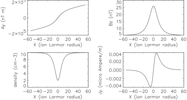
Figure 1 shows an example of a structure that is computed with pa-rameters typical of high altitude auroral plasmas : asymptotic magnetic field √ C = 3000 nT, n0 = 10cm −₃ , Ti = Te = 10 eV, and ηe= 1.53 10 −₁₆ (m/s)−₂ = 0.99ηc, very close to the critical value imposed by Eq. (28). A high

nega-tive value nc = −8cm−3 allows for a deep density depletion. The abcsissa is

normalized to the ion Larmor radius which is ρL = 152 m. We can see on

Fig. 1 that the size of the structure is about 4ρL ∼ 600 m. Such a narrow

and deep structure (the density in the cavity is only 20% of the density of the surrounding plasma) can be used in a first approximation for the density depletions encountered in the high altitude auroral zone.

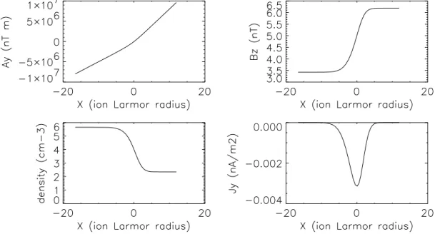
The solution displayed in Fig. 2 corresponds to the limiting case for η, obtained for the weakly magnetized interplanetary plasma encountered in the solar wind at one astronomical unit : √C = 5 nT, n0 = 10cm

−₃

, Ti = Te = 100 eV, and ηe = 1.53 10−17(m/s)−2 = 0.99ηc. The ion Larmor

radius is 280 km. We can notice that for the same density depletion, the variation of the magnetic field is much higher than in the case of a higly magnetized plasma. We also notice that the total size of the structure hardly exceed one ion Larmor radius.

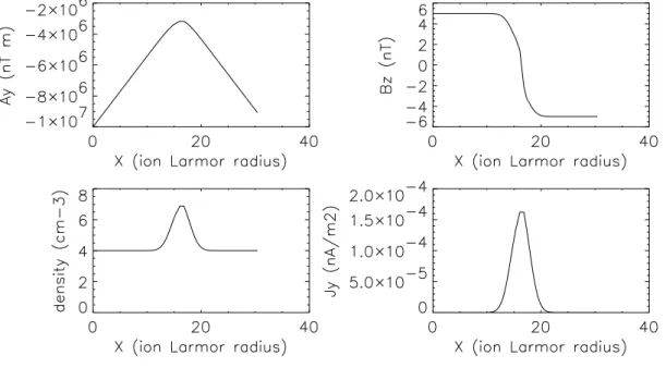
As the size is of the order of the ion Larmor radius, such solutions cannot be described through the fluid theories. Of course, we can also build very

large density structures, if we choose a small value of η in order to get a small value of ξ. Such large structures can more simply be described by fluid models. Figure 3 shows the solution with η = 10−₂₀

(m/s)−₂

∼ 10−₃

ηc. The

structure is much larger but has the same amplitude. Comparing Fig. 2 and Fig. 3, we can notice that, contrary to the case of solitons, there is no correlation between the size and the amplitude of the structures.

B. Asymptotic behaviour of the solutions

We can caracterize two kinds of non trivial elementary solutions : those with η 6= 0, and those where η = 0 (and therefore ν 6= 0, otherwise the solution is trivial). Those of the first kind correspond to localized solutions, they are centered around an abscissa x such as Ay(x) ∼ a. Therefore, when the

distribution is the infinite sum of elementary functions indexed by a as in Eq. (24), the parameter a indicates where the density na(x) is non negligible. Let

us consider an equilibria where, for x ∼ ∞, the magnetic field has a finite value. Then, the potential vector goes to infinity. Taking a1 ∼ −∞ and

a2 ∼ +∞ means that the plasma distribution will be influenced by some of

those elementary functions even when x ∼ ∞. On the contrary, equilibria defined with finite values of a1 and a2 (and B(∞) 6= 0) means that for x ∼ ∞,

the equilibria will converge toward the trivial solution of a uniform plasma with the density n0 that appears in Eq. (5).

The case of a null magnetic field at x ∼ ∞ (less useful for space plasmas applications) is different. Let us consider the case of B(+∞) = 0. For x ∼ +∞, the vector potential has a constant value. Let us call A∞this value.

Then, as A cannot exceed A∞, the main integral in Eq. (35) is divergent for

Ay(x) = A∞ (otherwise the equilibria would not be defined for any value of

x). As the elementary solutions parametrized by a are non negligible only for abscissas x such that Ay(x) is close to a, it is not necessary to consider

values or a2 that exceed notably A∞ : they would have no influence on the

value of the integral in Eq. (35). In brief, for equilibria with B(∞) = 0, the range of values where the parameter a is significant is bounded, a1 and a2 do

not have to be infinite.

In the Harris model, the magnetic field reverses and has two opposite finite values for x ∼ −∞ and x ∼ +∞. We shall see that there exist non elementary solutions where the magnetic field has finite values on both sides, and that these values have not necessarily the same absolute value.

We consider the case a1 = −∞ and a2 = +∞. Let u −

the limit of any physical value u when x tends to −∞, and u+ _{= lim}

x→+∞u.

The integral in Eq. (36), where y1 = −∞ and y2 = +∞ can be cut in three

parts : an integral I1 from y1 to x−Λ, an integral I2 from x−Λ to x+Λ, and

an integral I3 from x + Λ to y2. We will consider large values of x (positive

or negative), and large values of Λ.

For Λ large enough, y has large negative values,

I1 ∼

Z x−Λ

y1

dyB_z−k−_{exp (−ξ}−(B_z−)2_{(x − y)}2_{− δ}−B_z−_{(x − y))} (38) ∼ −k

−

δ−[exp δ −

B−_{Λ − exp δ}−B−y1] (39)

This function tends to zero for y1 → −∞ if δ − B− < 0, and diverges if δ− B− > 0. In the case δ− = 0, I1 ∼ Z x−Λ y1 dyB− z k − exp (−ξ− (B− z )2(x − y)2) (40)

tends toward zero. Similarily, limy1→−∞I3 = 0 if δ

+_B+_{≥ 0. With the same}

kind of technique, we can show that, for large negative values of x,

I2 ∼ k− s π ξ−σBz−exp (δ− )2 4ξ− , (41) where σ_B− z is the sign of B −

z. Provided that δ+B+ ≥ 0, and δ −

B−

≤ 0, the asymptotic expansion of Eq. (36) shows that

(B− z)2 = C + k − s π ξ−σ(B−z)exp (δ− )2 4ξ− . (42)

Computing an asymptotic value of I2 for x → +∞ bring a similar relation for (B+

z). The same method used with Eq. (37) provides the asymptotic

value of the contribution of each species to the particle density:

n+= n0+ N0+σ(B+z) s π ξ+exp (δ+₎2 4ξ+ . (43)

The equation for n−

is analogous. As dxn(∞) = 0, we deduce Jy+= J − y = 0.

There is no current density carried by the plasma for x ∼ ∞. This result can also be found with an asymptotic expansion of Eq. (31). Moreover, Eq. (31) shows that the ion and electron contribution to the current density have the same sign, their mean velocities are therefore opposite. As there is no current for x ∼ ∞, for each species v+ _{= v}−

= 0. The plasma does not flow perpendicularly to the magnetic field at x ∼ ∞.

C. Examples of solutions with and without field reversal

(m/s)−₂

close to ηc, ν = 0, and a function

ng(a) = 640atanh(1000a). The temperature is 10 eV. With C = (5nT )2,

the asymptotic magnetic field amplitude is 5nT. The ion Larmor radius is ρi ∼ 0.2 106m. The variable a is homogeneous to Bz times x, therefore

1000a ∼ x/ρi is of the order of magnitude of the absissa x divided by the

ion Larmor radius. The factor 640 that multiplies the inverse hyberbolic tangent function was set heuristically in order to get a variation of density of the order of 60%. The relatively low value of √C = 5 nT allows for high relative variations of the magnetic field amplitude. The asymptotic values of the magnetic field and of the density fit the analytical formulas given in section III.B.

Figure 5 shows an example where η = 0. We have chosen a function ng(a) = 4200e−(1000a)

2

. The temperature is 10 eV, and√C = 5 nT. The value ν = 10−₁₀

was chosen, because, in the exponential, the factor νa ∼ νBzx is

again of the order of x/ρi. We can see on Fig. 5 that the sign of the magnetic

field changes for x ∼ −∞ and x ∼ +∞. The reversal occur for a value of Ay that cancels the square root in Eq. (35). Although the magnetic field is

reversed on both sides, this is not a Harris equilibrium.

D. Example of a non isothermal plasma cavity in the

Earth auroral zone

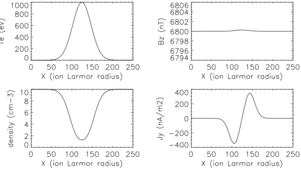
Are the cavities built in the Earth auroral zone in an equilibrium state of the plasma ?

Hilgers et al. [1] made a careful analysis of the Langmuir probe current measurements onboard the swedish Viking satellite in low plasma densities. They showed a case, taken at an altitude of 7000 km, of a deep auroral cavity. The density reach less than one particle per cubic centimeter, that is less than 10 % of the surrounding plasma density. The electron plasma temperature in the cavity (although not precisely measured) is of the order of 1 keV, compared to 1 eV outside the cavity. The boundaries of the cavity are sharp, Hilgers et al. measured 1.4 km, of the order of a few ion Larmor radii. The magnetic field amplitude is Bz0 = 6800 nT.

qual-itatively reproduced in the elementary equilibria shown in Fig. 1. In or-der to reproduce a cavity with sharp temperature gradients, an elemen-tary solution cannot be used. Let ρi be the Larmor radius outside the

cavity, it corresponds to the cold palsma (1 eV), its value is 21 m. In-side the cavity, the plasma temperature is 1 keV, and the ion Larmor ra-dius is ρi,hot = 660m= 32ρi. We choose an electron temperature function

Te(a) = 1 + 1000 exp (−(a/Bz032ρi)2) that varies from 1 to 1000 eV on a

scale ∆x ∼ 32ρi ∼ ρi,hot. The density is controled through the constant

scalar n0 = 10 cm −₃

, and the ng function, ng(a) = −ng0exp (−(a/Bz032ρi)2).

The scalar ng0 is set (heuristically) to 50000 in order to have one particle per

cubic centimeter inside the cavity. The ν function is null. The η function is chosen is order to get a sharp cavity, that is with a value close to the ηc

func-tion: η(a) = 0, 98ηc(a) have values of the order of 10 −₁₅

(m/s)−₂

. Actually, the equilibria is not very sensitive on the value of η. Taking a lower value like η(a) = 0.7ηc(a) (and a slightly lower value of ng0) bring similar results.

The result, displayed on Fig. 6, is in quantitative agreement with the prescriptions given by the observations. The size of the gradient is 70ρi =

1400m, as measured by Hilgers et al.

We can notice on figure 6 that the magnetic field amplitude variation ∆B in the cavity is about 0.5 nT. A similar equilibria (not displayed) set with a lower value of the ambient magnetic field (Bz0 = 300 nT) bring a larger

variation: ∆B = 5 nT.

We conclude from this short study that deep plasma cavities can be equi-librium structures of the Earth auroral plasma. Therefore, they won’t be destroyed immediately after the extinction of their cause. It is however in-teresting to know if this equilibrium is stable. The theoretical treatement of this question goes beyhond the scope of this paper. I will only give a few hints in favour of the stability of the auroral cavities.

The Auroral zone of the Earth is a radio source. The power of the emis-sions, called Auroral Kilometric Radiation (AKR), can reach 10 MW. The Viking spacecraft has gone through the sources of AKR: the waves are emit-ted inside the cavities, where they take their free energy from the hot rarefied plasma [7]. The waves are strongly refracted at the edges of the AKR source, and it is probable that a part of the AKR is guided inside the cavities [14]. Auroral kilometric radiations can be observed on time scales of 10 minutes. The cavities that contain AKR sources are expected to last at least for the same duration. Therefore, two situations are possible : (1) the cavities are the consequence of a phenomena that lasts for tens of minutes, or (2) they

are generated by more transient phenomena and they are stable.

An another hint about the stability of hot plasma cavities comes from numerical simulations carried by Genot et al. [9]. The simulations start with an isothermal (a few eV) auroral cavity. The cavity is stable. An Alfv´en wave is added. The interaction of the Alfv´en wave with the cavity triggers strong electron acceleration and turbulence. When the free energy is completely removed from the Alfv´en wave by the accelerated electrons, the plasma inside the cavity is hot, and the surrounding plasma is cold. We are in the situation shown in Fig 6. The simulations show that the heated cavity, which is still very deep and sharp, is stable.

Most of the models about the generation of auroral cavities invoke strong kinetic Alfv´en Waves (SKAW) [15] [16], observed onboard the Freja and FAST satellites [17], [18]. The associated magnetic field perturbation ∆B is of the order of 50 nT. But the observations made onboard FAST show that the SKAW’s are mainly observed in the cusp and the polar cap boundary layer, while the cavities are observed in the lower latitude auroral region where the magnetic fluctuations ∆B do not exceed 5 nT. It is possible that the cavities are built in the polar cap boundary layer by SKAWs, they subsist after the disapearance of the Alfv´enic perturbations and finally they are gently convected to lower latitudes by the large scale convection electric field. This suppose of course the stability of the auroral cavities. An other scenario is that the cavities are created through Field Line Resonance (FLR) [19] directly in the auroral region. The ∆B ∼ 5 nT (on a time scale that corresponds to the crossing of a cavity by a spacecraft) associated to the FLR is compatible with the value shown in Fig. 6. The equilibria shown in Fig. 6 may be a relevant short scale Vlasov-Maxwell description of the part of the FLR that is in the high altitude auroral zone (the FLR has been modeled on a global scale in the multifluid approximation up to now).

IV. CONCLUSION AND FURTHER

DEVLOPP-MENTS

This paper presents a large class of monodimensional analytic kinetic equi-libria. They are based on particle distribution functions Eq. (5) that depend on a set of almost arbitrary functions. These distribution functions are so-lutions of the Vlasov equation, and the vector potential can be computed

through the evaluation of the integral function given in Eq. (35). In some particular cases, like the uniform plasma and the Harris current sheet, this integral is a combination of elementary mathematical functions. In the other cases, its numerical evaluation is straightforward.

Unlike most of the kinetic tangential equilibria given in the litterature, the freedom in the choice of the density profile, altough more difficult to control, is almost as large as with bi-fluid models. The kinetic equilibria have the great advantage of giving a complete description of the distribution function (not provided with the fluid theory), and can describe equilibria where strong gradients develop on the scale of a few ion Larmor radii. These solutions can be used as initial conditions in particle in cell and Vlasov numerical simulations.

Most of the authors who build models and are cited in this paper have based their elementary solutions on distribution functions that depend on the invariants of the motion. Some of them combined a small number of such elementary solutions and asserted that each of these elementary solutions correspond to a family of trapped particles. The distribution function given in Eq. (5) is the superposition, not of a finite number, but of a continuum of families of trapped particles. This is why we have a very large degree of freedom in the choice of the density and temperature profiles. For the first time, we show that such a supperposition of families of trapped particles lead to an analytically integrable equation, whose solution is given in Eq. (35)

The equilibria discussed in section III.B where the plasma is uniform for x ∼ ∞ can be compared to the solutions of the jump equations developed in the frame of the MHD theory. The equilibria developed in the present paper are characterized by jumps of the density and of the magnetic field, the normal velocity is null as well as the normal magnetic field. They therefore belong to the family of tangential discontinuities. But they concern only a sub-category: the magnetic field direction is uniform and the solutions have no velocity shear: the velocities are equal to zero at x ∼ −∞ and x ∼ +∞, even if they can take other values at finite distances. These restrictions are not required for general tangential discontinuities.

Building a kinetic model, inspired from the present results, of a tangential discontinuity where the magnetic field can turn is straighforward and will be presented in a forthcomming paper in order to analyse experimental data provided by the Cluster satellites.

A kinetic model of a tangential equilibria whith a velocity shift (x ∼ −∞ and x ∼ +∞) is not compatible with exact charge neutrality. A quasi neutral

model would do. It could be computed, as a first order perturbation in ni−ne

added to the charge neutral equilibria presented in this paper.

The examples given in the present paper come from the magnetospheric and solar wind physics because these media offers the opportunity of in situ observations of non collisional astrophysical plasmas. Tangential equilibria can be used to describe the magnetopause (present around all the magnetized planets with an atmosphere), the distant neutral sheet, the Earth auroral cavities, and some density fluctuations of the solar wind [20].

But tangential equilibria do not exist only in the terrestrial environnment. They exist whenever plasmas with different origins and velocities meet. Such situations exist in many astrophysical plasmas. Theoretical models (based on MHD and plasma multifluid theories) of the boundary of the Heliosphere show that it is constituted of a termination shock, followed by the heliopause, that is a tangential discontinuity, an hydrogen wall, and possibly an helio-spheric shock [21]. Tangential discontinuities also exist around other stars. M¨uller et al. [22] studied the interaction of the very active binary star λ An-dromedae, and of the neaby star ǫ Indi with the interstellar medium. They found, as in the case of the heliopause, the existence of four boundaries, one of them, the asteropause being a tangential discontinuity. It is clear that tangential layers exist in other astrophysical plasmas where they may play a very important role, as frontiers, or in acceleration, heating and radiative processes.

The studies of the magnetospheric plasmas have shown that most of the heating and acceleration phenomena can be only explained through kinetic processes. So far, most of the remote astrophysical plasmas have been stud-ied through MHD or multifluid theories. The understanding of acceleration processes in remote astrophysical plasma might as well require kinetic mod-els. The equilibria presented in this paper might be a good start for some of those studies.

ACKNOWLEDGMENTS

The author gratefully acknowledges stimulating and usefull discussions with G´erard Belmont and Alain Roux.

References

[1] Hilgers, A.,B. Holback, G. Holmgren, and R. Bostr¨om, J. Geophys. Res. 97, A6, 8631, (1992).

[2] Strangeway R.J., L. Kepko, R.C. Elphic, C.W. Carlson, R.E. Ergun, J.P. McFadden, W.J. Peria, G.T.Delory, C.C.Chaston, M. Temerin, C.A. Cat-tell, E. M¨obius,L.M. Kistler, D.M. Klumpar, W.K. Peterson, E.G. Shelley, and R. Pfaff, Geosphys. Res. Let., 25, 12, 2065, (1998).

[3] J.P. McFadden, C.W. Carson, R.E. Ergun, C.C. Chaston, F.S. Mozer, M. Temerin, D. M. Klumpar, E.G. Shelley, W.K. Peterson, E. Moebius, L. Kistler, R. Elphic, R. Strangeway, C. Cattell, R. Pfaff Geophys. Res. Lett., 25, 12, 2045, (1998).

[4] Hilgers, A., Geophys. Res. Lett., 19 3, 237-240, (1992).

[5] G´enot, V., P. Louarn, and D. Le Qu´eau, A study of the propagation of Alfv´en J. Geophys. Res. 104 22,649, (1999).

[6] V. G´enot, P. Louarn, and F. Mottez, JJ. Geophys. Res. 105, A12, 27611, (2000).

[7] A. Roux, A. Hilgers, H de Feraudy, D. Le Queau, P. Louarn, S. Perraut, A. Bahnsen, M. Jesperen, E. Ungstrup, M. Andre, J. Geophys. Res., 98, 11657, (1993).

[8] R. Pottelette, R.A. Treumann, M. Berthomier, J. Geophys. Res., 106, 8465, (2001).

[9] V. G´enot, P. Louarn, and F. Mottez, J. Geophys. Res. 106, A12, 29633, (2001).

[10] E.G. Harris, Il Nuovo Cimento 23 1, 115, (1962). [11] P. J. Channell, Phys. Fluids 19 10, 1541, (1976).

[12] M. Roth, J. De Keyser, M.M. Kuznetova, Space Sci. Rev., 76, 251, (1996).

[14] de Feraudy,H., B.M. Pedersen, A. Bahnsen, and M. Jespersen, Geophys. Res. Lett., 14 511, 1987.

[15] Wu,D.J., D.Y. Wang, and G.L. Huang, Phys. Plasmas, 4 (3), 611, (1997).

[16] Shukla, P.K., L. Stenflo, R. Bingham, Phys. of Fluids, 6, 5, 1677, (1999). [17] Louarn, P., J.E. Wahlund,T. Chust, H de Feraudy and A. Roux, B. Holback, P.O. Dovner, A.I. Eriksson and G. Holmgren, Geophys. Res. Lett., 21, 17, 1847, (1994).

[18] Chaston, C.C., C.W. Carlson, W.J. Peria, R.E. Ergun and J.P. Mc Fadden, Geophys. Res. Lett. 26,6, 647, (1999).

[19] Lotko,W., A.V. Streltsov, C.W. Carlson, Geophys. Res. Lett., 25, 24, 4449, (1998).

[20] Safrankova, J., Prech, L., Nemecek, Z., Sibeck, D.G. Mukai, T, J. Geophys. Res., 105, 11, 25113, (2000).

[21] Zank, G.P., Space Sci. Rev., 89, 413, (1999).

Figure 1: FIG. 1. A deep and narrow density depletion in a highly magne-tized plasma. The parameters of this equilibrium are given in Sec. III.A.

Figure 2: FIG. 2. A deep and narrow density depletion plasma with a weak magnetic field. The parameters are the same as for Fig. 1, exepct for C that

Figure 3: FIG. 3. A deep and large density depletion, the only difference with Fig. 2 is a larger value of η. See Sec. III.A..

Figure 4: FIG. 4. An example of non symetric equilibrium where ng is a

Figure 5: FIG. 5. An exemple of an equilibrium with η = 0 and a reversal of the magnetic field. Details are given in Sec III.C.

Figure 6: FIG. 6. An example of a deep plasma cavity containing hot elec-trons (1 keV) surrounded by a cold (1 eV) highly magnetized plasma. See