HAL Id: hal-00317042
https://hal.archives-ouvertes.fr/hal-00317042
Submitted on 1 Jan 2003
HAL is a multi-disciplinary open access
archive for the deposit and dissemination of
sci-entific research documents, whether they are
pub-lished or not. The documents may come from
teaching and research institutions in France or
abroad, or from public or private research centers.
L’archive ouverte pluridisciplinaire HAL, est
destinée au dépôt et à la diffusion de documents
scientifiques de niveau recherche, publiés ou non,
émanant des établissements d’enseignement et de
recherche français ou étrangers, des laboratoires
publics ou privés.
channel (AWFC) observed during a magnetospheric
substorm
M. L. Parkinson, M. Pinnock, H. Ye, M. R. Hairston, J. C. Devlin, P. L.
Dyson, R. J. Morris, P. Ponomarenko
To cite this version:
M. L. Parkinson, M. Pinnock, H. Ye, M. R. Hairston, J. C. Devlin, et al.. On the lifetime and extent
of an auroral westward flow channel (AWFC) observed during a magnetospheric substorm. Annales
Geophysicae, European Geosciences Union, 2003, 21 (4), pp.893-913. �hal-00317042�
On the lifetime and extent of an auroral westward flow channel
(AWFC) observed during a magnetospheric substorm
M. L. Parkinson1, M. Pinnock2, H. Ye3, M. R. Hairston4, J. C. Devlin3, P. L. Dyson1, R. J. Morris5, and P. Ponomarenko6
1Department of Physics, La Trobe University, Victoria 3086, Australia
2British Antarctic Survey, Natural Environment Research Council, Cambridge CB3 0ET, UK 3Department of Electronic Engineering, La Trobe University, Victoria 3086, Australia
4William B. Hanson Center for Space Sciences, University of Texas at Dallas, Richardson, Texas, USA 5Australian Antarctic Division, Kingston, Tasmania 7050, Australia
6Department of Physics, University of Newcastle, New South Wales 2038, Australia
Received: 6 May 2002 – Revised: 24 October 2002 – Accepted: 8 November 2002
Abstract. A −190-nT negative bay in the geomagnetic X
component measured at Macquarie Island (−65◦3) showed that an ionospheric substorm occurred during 09:58 to 11:10 UT on 27 February 2000. Signatures of an auroral westward flow channel (AWFC) were observed nearly si-multaneously in the backscatter power, LOS Doppler ve-locity, and Doppler spectral width measured using the Tas-man International Geospace Environment Radar (TIGER), a Southern Hemisphere HF SuperDARN radar. Many of the characteristics of the AWFC were similar to those occur-ring duoccur-ring a polarisation jet (PJ), or subauroral ion drift (SAID) event, and suggest that it may have been a pre-cursor to a fully developed, intense westward flow channel satisfying all of the criteria defining a PJ/SAID. A beam-swinging analysis showed that the westward drifts (pole-ward electric field) associated with the flow channel were very structured in time and space, but the smoothed veloc-ities grew to ∼800 m s−1 (47 mV m−1) during the 22-min substorm onset interval 09:56 to 10:18 UT. Maximum west-ward drifts of >1.3 km s−1(>77 mV m−1) occurred during a ∼5-min velocity spike, peaking at 10:40 UT during the ex-pansion phase. The drifts decayed rapidly to ∼300 m s−1 (18 mV m−1) during the 6-min recovery phase interval, 11:04 to 11:10 UT. Overall, the AWFC had a lifetime of 74 min, and was located near −65◦3in the evening sector west of the Harang discontinuity. The large westward drifts were confined to a geographic zonal channel of longitudinal ex-tent >20◦(>1.3 h magnetic local time), and latitudinal width
∼2◦3. Using a half-width of ∼100 km in latitude, the peak electric potential was >7.7 kV. However, a transient velocity of >3.1 km s−1with potential >18.4 kV was observed fur-ther poleward at the end of the recovery phase. Auroral oval boundaries determined using DMSP measurements suggest Correspondence to: M. L. Parkinson
(m.parkinson@latrobe.edu.au)
the main flow channel overlapped the equatorward bound-ary of the diffuse auroral oval. During the ∼2-h interval following the flow channel, an ∼3◦3wide band of scatter was observed drifting slowly toward the west, with speeds gradually decaying to ∼50 m s−1 (3 mV m−1). The scatter was observed extending past the Harang discontinuity, and had Doppler signatures characteristic of the main ionospheric trough, implicating the flow channel in the further depletion of F-region plasma. The character of this scatter was in con-trast with the character of the scatter drifting toward the east at higher latitude.
Key words. Ionosphere (auroral ionosphere; electric fields
and currents; ionosphere-magnetospehere interactions) Mag-netospheric physics (storms and substorms)
1 Introduction
Transient (∼1 h), supersonic (>1 km s−1) westward flows of
ionospheric plasma are sometimes observed confined within narrow latitudinal channels (<2◦) just equatorward of, or
overlapping, the equatorward edge of the diffuse auroral oval in the evening sector (∼22 h magnetic local time; MLT) (e.g. De Keyser, 1998). These events were originally called polar-isation jets (PJs) by their discoverers, Galperin et al. (1973), but have also become known as subauroral ion drift events (SAIDs) (Spiro et al., 1979), despite the fact that SAIDs of-ten overlap the diffuse auroral oval. Most observations of PJ/SAIDs have been made using instruments on board satel-lites (e.g. Smiddy et al., 1977; Rich et al., 1980; Anderson et al., 1991, 1993; Karlsson et al., 1998), but a few ground-based radar observations have also been reported (Galperin et al., 1986; Providakes et al., 1989; Yeh et al., 1991).
In this paper we report observations of an auroral west-ward flow channel (AWFC) observed at ∼22:00 MLT and
magnetic latitude ∼−65◦3 on 27 February 2000.
Signa-tures of the event appeared in the backscatter power (dB), line-of-sight (LOS) Doppler velocity (m s−1), and Doppler spectral width (m s−1) measured using the Tasman Interna-tional Geospace Environment Radar (TIGER) (Dyson and Devlin, 2000), a Southern Hemisphere member of the Super Dual Auroral Radar Network (SuperDARN) (Greenwald et al., 1985, 1995). The behaviour of the AWFC resembled the behaviour of a relatively weak PJ/SAID, yet its growth and decay were synchronised with substorm onset and recovery, respectively. In this regard, the AWFC more closely resem-bled the substorm-associated radar auroral surges (SARAS) observed using VHF radar in the afternoon sector (Freeman et al., 1992).
This study reports HF radar observations of a class of rela-tively weak, subauroral westward flow channels that has ap-parently been excluded from previous satellite-based studies. The behaviour of AWFC, SARAS, and PJ/SAID needs to be understood in the context of other poorly understood sub-storm processes which have been investigated in numerous other studies. For example, a study by S´anchez et al. (1996) is especially relevant here because of its comprehensive syn-thesis of HF radar, magnetometer, and Defence Meteoro-logical Satellite Program (DMSP) observations. Although we cannot be certain that our 27 February event was not driven by nightside reconnection, its persistent character and probable mapping to a region of closed field lines suggests that it was more closely related to PJ/SAIDs. To this end, we first review recent observations and theory pertaining to PJ/SAIDs.
2 PJ/SAID review
Anderson et al. (1991) studied PJ/SAIDs using Atmospheric Explorer C and Dynamics Explorer B spacecraft measure-ments. They defined PJ/SAIDs as having westward drifts of at least 1 km s−1, with velocities up to 4 km s−1often occur-ring in the evening sector. However, weaker PJ/SAID-related drifts <1 km s−1must also occur, though with more structure (Karlsson et al., 1998). Anderson et al. (1993) observed flow channels with full-width half-maxima of ∼1◦in latitude, and estimated life times in the range 30 min to 3 h, commenc-ing durcommenc-ing the substorm recovery phase. They did not ob-serve any events within 30 min of substorm onset, but their results were not definitive due to intermittent satellite sam-pling. Karlsson et al. (1998) provided a comprehensive ac-count of PJ/SAID occurrence statistics compiled using Freja satellite data.
Anderson et al. (1991) also observed large enhancements in the ionospheric ion temperature, upward vertical drift, and associated depletions in low-altitude ion density. These are the familiar consequences of ion-neutral friction foreseen by Schunk et al. (1975), and modelled by Sellek et al. (1991) and Heelis et al. (1993). The O+and O+2 recombination rates are elevated when the difference between the ion and neutral speeds is large. When the ion speed suddenly increases and
persists for ∼10–15 min, the frictional heating can lead to the formation of deep depletions in ionospheric plasma concen-tration. The frictional heating may also lead to the formation of a stable auroral red arc (Foster et al., 1994).
Anderson et al. (1991) reported PJ/SAIDs collocated with the poleward edge of the main ionospheric trough, lead-ing to the formation of very deep depletions inside the pre-existing trough, presumably formed by stagnation (e.g. Que-gan et al., 1982; Sojka and Schunk, 1989; Rodger et al., 1992). These are the “troughs within troughs” reported by Galperin et al. (1986). Incoherent scatter radar observations show troughs are often narrow latitudinal features, only ∼1◦ wide (Jones et al., 1997). PJ/SAIDs may also cause notice-able plasma depletions at plasmaspheric altitudes (Ober et al., 1997). Clearly, there is an intimate relationship between PJ/SAIDs, the formation of high-latitude troughs, the loca-tion of the plasmapause, and the structure within the high-altitude plasma trough.
Southwood (1977) gave a fluid description of the shield-ing of the low-latitude ionosphere from convection electric fields. During a geomagnetic storm, the dawn-to-dusk elec-tric field causes an earthward drift of plasma in the mag-netotail. If unimpeded, this would map to purely sunward flows migrating all the way down to the equatorial iono-sphere. However, the earthward-drifting plasma clouds en-counter radial pressure gradients approaching the inner edge of the ring current (near the plasmapause), whereupon east-west gradients in plasma pressure grow. These gradients di-vert the plasma flow in the zonal direction, thereby shielding the plasmasphere (mid-latitude ionosphere) from the cross-tail electric field. In the co-rotating frame, these zonal drifts are slowly toward the east post-midnight, but strongly toward the west pre-midnight.
Southwood (1977) suggested the hot plasma pressure, its number density in the inner nightside magnetosphere, and the ionospheric conductivity are the key parameters controlling the penetration of convection electric field to low latitude. This is because the magnetospheric convection will tend to avoid expending energy in plasma compression and Joule heating (Cole, 1962) in magnetically connected regions of large ionospheric conductivity (Axford, 1969). These ideas suggest that PJ/SAIDs will inevitably manifest in the iono-spheric region mapping to just outside the sharp pressure gra-dients located near the plasmapause, yet just equatorward of the highly conducting auroral zone. PJ/SAIDs will persist until there is no longer an equilibrium between the coupled magnetosphere-ionosphere forces generating the polarisation field, and the shorting out of this field by field-aligned cur-rents closing via ionospheric Pedersen curcur-rents (and the as-sociated Joule heating).
Any PJ/SAID theory must explain the formation of an in-tense, spatially localised polarisation field directed poleward in the ionosphere, and radially in the inner magnetosphere. Invoking a magnetospheric driver, there must be a radial sep-aration of the ion and electron ring currents, with more ions located closer to Earth. Anderson et al. (1993) suggested that PJ/SAID do not form at the time of substorm onset
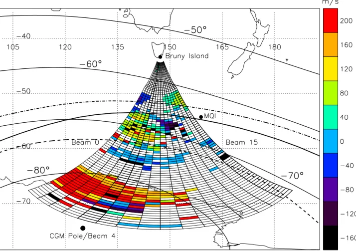
be-Fig. 1. Field of view (FOV) of the TIGER radar mapped to cylindrical geographic coordinates with AACGM latitudes −50◦, −60◦, −70◦, and −80◦3superimposed. Beam 4, which points toward the CGM pole, and beam 15, which becomes a magnetic zonal beam at the furthest ranges, are shown in bold. LOS Doppler velocities recorded during the full scan commencing at 12:34 UT on 27 February 2000 are also shown. The colour key means that all velocities in the range 140 < vLOS≤180 m s−1are coloured orange. Auroral oval boundaries given
by the Starkov (1994) model for AL = −150 nT and Macquarie Island (MQI) located at 22:00 MLT have been superimposed: poleward boundary of discrete aurora (dashed curve), the equatorward boundary of discrete aurora (solid curve), and the equatorward boundary of diffuse aurora (dashed-dotted curve).
cause ion and electron precipitation share a common, disper-sionless, equatorward boundary (Newell and Meng, 1987). Thereafter, the inner edges of the ion and electron plasma sheets separate on a time scale of ∼10 min, with the hot ions moving further earthward than the hot electrons in the evening sector as the Alfv´en layer forms (Kivelson and Rus-sel, 1995). This leads to the formation of an initial radial polarisation field. Since the hot ions are injected near mid-night first, and then drift westward in the ring current, we might also expect the ionospheric signature of PJ/SAIDs to expand westward from the Harang discontinuity.
Anderson et al. (1993) also emphasised the importance of ion-neutral frictional heating in the ionosphere, leading to a reduction in plasma density and thus conductivity. As long as the magnetospheric driver supplies the same field-aligned current closing via Pedersen current in the iono-sphere (Jp =6pE), a runaway effect develops: the electric
field, E, increases, leading to a further decrease in height-integrated conductance, 6p, leading to a further increase in
the electric field, etc. Hence, narrow, westward drifts may rapidly grow to >4 km s−1at subauroral latitudes during sub-storms.
De Keyser (1999) argued the space-charge layer associ-ated with the Alfv´en layer is too thick to explain the narrow latitudinal width of PJ/SAIDs. He proposed that an intense radial electric field is generated by a thermoelectric effect, namely a strong temperature gradient develops across the interface between cold, plasma trough plasma (Telectrons ≈
0.75 eV; Tprotons ≈ 1.5 eV) and hot, plasma sheet plasma
(Telectrons ≈1 keV; Tprotons ≈ 10 keV), the latter injected at
substorm onset. Space-charge separation develops because the various particles with different energies have different gyroradii. The azimuthal flow shear between the partially co-rotating plasma near the plasmapause and the newly injected plasma must also be considered: the hot plasma drifts west-ward pre-midnight and eastwest-ward post-midnight. Hence, the flow-shear electric field reinforces the thermoelectric field in the evening sector, but suppresses it in the morning sector.
This explains the strong preference for PJ/SAIDs to occur in the evening sector.
The semi-quantitative model of PJ/SAIDs recently pro-posed by Galperin (2002) considers the distribution functions of ion and electron energies injected into the ring current region. Galperin (2002) argued that (1) the formation time of a PJ/SAID will be ∼5–10 min, (2) the initial injection will be near the tip of the Harang discontinuity, which will be displaced by several hundred km, (3) the latitudinal pro-file of enhanced poleward electric field will be bell-shaped with a width of ∼100 km (∼1◦), (4) an electric potential
of ∼10 kV will map over the same distance, (5) the Ped-ersen conductance 6p will be ∼0.1 S (versus ∼10 S in the
auroral oval) and a height-integrated Pedersen current den-sity ∼10−2A m−1will flow across the PJ, (6) the lifetime of the PJ/SAID will be ∼1–3 h, and (7) the PJ/SAID will extend for at least 3 h in MLT. This recipe for a PJ/SAID agrees with numerous satellite observations, but needs further testing.
Spacecraft observations have provided important insights into the spatial extent and timing of PJ/SAIDs relative to sub-storm processes. Satellites have obtained high-time resolu-tion measurements of PJ/SAID processes along single orbits traversing the events. However, due to the typical orbital pe-riod of ∼90 min for satellites in the topside ionosphere, the effective time resolution and spatial coverage is poor when a satellite encounters the same event during a subsequent or-bit. No doubt this problem will be addressed in future exper-iments deploying large clusters of “nano-satellites”. Mean-while, ground-based HF backscatter radar observations offer an excellent opportunity to image PJ/SAID processes occur-ring almost continuously in space and time.
In this paper, we report comprehensive observations of an AWFC made using a HF radar supported by coincident spacecraft measurements. By an AWFC we simply mean a PJ/SAID-like event with well above average westward drifts overlapping or residing within the auroral oval and possibly synchronised to substorm dynamics. We suggest that AWFC, SARAS, and PJ/SAIDs are governed by closely-related elec-trodynamic processes occurring during substorms.
3 Observations and interpretation
TIGER (Dyson and Devlin, 2000) is a SuperDARN radar (Greenwald et al., 1985, 1995) located on Bruny Island (43.4◦S, 147.2◦E geographic), Tasmania (Fig. 1). Under
routine operation, TIGER performs one sequential 16-beam scan from east (beam 15) to west (beam 0), integrating for 7 s on each beam. Hence, a full scan takes 112 s, but succes-sive scans are synchronised to the start of 2-min boundaries. The individual beams are separated by 3.24◦, so the full scan is 52◦wide (though decreasing slightly with increasing fre-quency). The radar samples 75 different ranges separated by 45 km between 180 and 3555 km. In practise, the radar de-tects useful ionospheric scatter from a fraction of the field of view (FOV) during a single scan. Nonetheless, the radar
potentially detects scatter from ∼106km2of the ionosphere every 2 min.
Figure 1 shows that TIGER beam 4 observation cells ex-tend from magnetic latitude −57◦3 to −88◦3, which is ∼5◦3 equatorward of the high-latitude ionosphere imaged by most SuperDARN radars. Hence, TIGER’s location is optimum for the study of substorm-related processes in the nightside ionosphere during quiet and moderate geomagnetic activity. Here we report routine HF radar observations of an AWFC located at ∼−65◦3, and commencing at 09:56 UT (22:00 MLT) on the evening of 27 February 2000. The obser-vations were made using the routine, 2-min full-scan sound-ing mode, as previously described.
The line-of-sight (LOS) Doppler velocities (m s−1) (vLOS)
recorded during the 112-s interval commencing at 12:34 UT on 27 February, 2000 have been superimposed in Fig. 1. Note the absence of near-range scatter on beams 4 to 8. As will be discussed, the ionospheric irregularities drifted slowly (<100 m s−1) toward the west equatorward of ∼−66◦3, and were probably associated with the main ionospheric trough. Immediately poleward, the irregularities drifted with moder-ate speed (>100 m s−1) toward the east, thereby delineating the location of the flow reversal boundary (FRB) (Huang et al., 2001). The AWFC preceded this observation and was part of the process forming the FRB near the equatorward edge of the auroral oval.
We relate our TIGER observations to the timing of au-roral substorms inferred from magnetometer observations made at nearby Macquarie Island (MQI) (54.5◦S, 158.9◦E; −65◦3). Interpretation of the observations was supported by coincident Wind and Interplanetary Monitoring Plat-form 8 (IMP 8) solar wind measurements, Defence Meteo-rological Satellite Program (DMSP) precipitation measure-ments, Los Alamos National Laboratory (LAN-L) geosyn-chronous (6.6 RE) spacecraft measurements of energetic
par-ticle fluxes, ionosonde measurements made at MQI, and total electron content (TEC) measurements made at MQI and Ho-bart (42.9◦S, 147.3◦E; −54◦3).
3.1 Solar wind observations
At 10:00 UT on 27 February 2000, the IMP 8 spacecraft was located below the equatorial plane on the dusk flank of the magnetosphere at geocentric solar magnetospheric (GSM) x, y, and z coordinates of −2.7, 36.5, and −18.8 RE,
respec-tively. Figure 2 shows IMP 8 measurements (bold lines with solid dots) of the interplanetary magnetic field (IMF) com-ponents in GSM coordinates (parts a–c), and simultaneous measurements of the solar wind dynamic pressure (part d). There were substantial outages in measurements made with the ageing IMP 8, so continuous Wind spacecraft measure-ments of the same parameters are included (faint curves). At 10:00 UT, the Wind spacecraft was located much further up-stream in the solar wind at GSM coordinates (173.9, 30.3, 17.4 RE). The Wind measurements were advanced in time
by 33.5 min to allow for advection of the IMF conditions from Wind to IMP 8 at a representative solar wind speed of
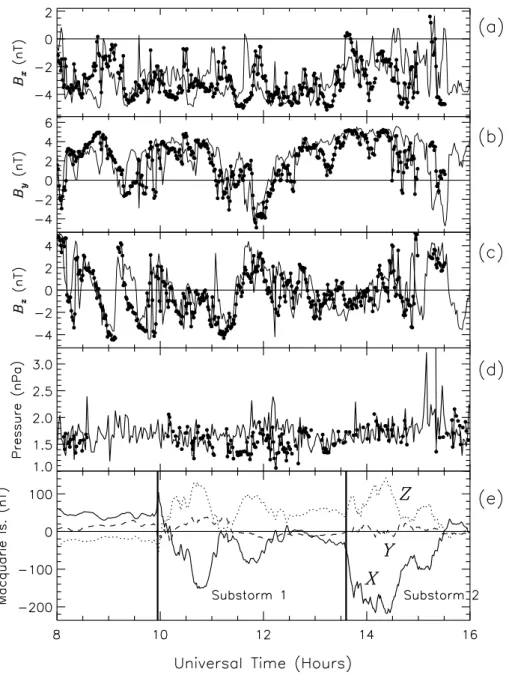
Fig. 2. IMP 8 spacecraft measurements (bold lines with solid dots) of the IMF (a) Bx, (b) By, and (c) Bzcomponents made at ∼1-min time
resolution, and (d) the solar wind dynamic pressure during 08:00 to 16:00 UT on 27 February 2000. The corresponding Wind spacecraft measurements made at ∼1.5-min time resolution for the same period, except advanced by 33.5 min to allow for advection of the solar wind to the location of IMP 8, are superimposed as faint curves. (e) Perturbations of the geomagnetic X (solid curve), Y (dashed curve), and Z (dotted curve) components measured by the MQI magnetometer (data provided courtesy of the Australian Geological Survey Organisation). The abscissas have tick marks at 30-min intervals of UT.
560 km s−1. To reduce clutter in the plot, ACE spacecraft measurements are not shown.
The IMP 8 and Wind IMF measurements agreed in the ba-sic trends occurring on time scales >15 min, but there were many differences occurring on shorter time scales. These were partly caused by instrumental errors, evolution of the solar wind, and by discontinuities and waves propagating at much higher speed within the background flow. Clearly, a spacecraft with reliable instruments deployed nearby the Earth’s magnetosphere provides the best indication of geo-effective solar wind conditions. In summary:
1. The IMF Bx component was continuously fluctuating,
mostly in the range −1 to −5 nT.
2. By was predominately positive in the range 2 to 5 nT,
but with significant negative excursions during 09:17 to 09:55 UT, and especially 11:04 to 12:13 UT.
3. Bz was predominately negative in the range −1 to
−4.5 nT, but with many northward excursions, too nu-merous to warrant separate listing.
4. Excluding continuous short-term fluctuations, the solar-wind dynamic pressure was reasonably steady at around 1.7 nPa. However, significant changes in pressure (∼35%) occurred at 11:46 and 12:11 UT, and large pres-sure pulses (>88%) occurred at 15:09 and 15:20 UT. 3.2 Ground-based magnetometer observations
Macquarie Island (MQI) (−65◦3) is located just east of TIGER beam 15, having the same magnetic latitude as range cell 26 (1350 km) (Fig. 1). Figure 2e shows MQI magne-tometer perturbations in the geomagnetic X (north), Y (east), and Z (down) components. These measurements were de-spiked and then detrended by subtracting a baseline defined by their average diurnal values. The two largest negative bays in the X component exhibited the classic signatures of iono-spheric substorms. We have labelled them “Substorm 1” and “Substorm 2,” but lesser intensifications occurred, just after both substorms.
Substorm 1 was not preceded by an obvious growth-phase signature (McPherron, 1970). Rather, its onset was marked by an ∼60-nT impulsive increase in the X component, start-ing at 09:53 UT, and peakstart-ing at 09:58 UT (bold vertical line). This feature was reminiscent of storm sudden commence-ment (ssc), a feature normally observed in dayside magne-tograms when magnetopause currents are enhanced by mag-netospheric compression (Kelley, 1989). However, the be-haviour of the IMF Bz component does not suggest
unusu-ally enhanced dayside reconnection; nor was there a signifi-cant dynamic pressure pulse at this time. Hence, the feature suggests a strong, short-lived current flowing toward the east, opposite to the ring current. We will argue this feature was a signature of an emerging AWFC.
Substorm 1 was possibly triggered by Bzswinging
north-ward after a preceding succession of Bz southward turnings
(Fig. 2c). We expect a very short delay for the ionosphere to respond to IMF conditions measured at GSM x = −2.7 RE.
There were several intensifications in the X component dur-ing the onset and expansion phase, reachdur-ing a maximum deflection of −190 nT relative to our pre-storm baseline. The recovery phase commenced at 10:53 UT, and finished at 11:10 UT. A lesser intensification to −83 nT began near 11:28 UT, and was possibly driven by a lesser Bzsouthward
turning.
Substorm 2 had stronger Hall current flow than Substorm 1. The growth-phase signature in the X component be-gan at 12:43 UT, if not earlier, possibly in response to Bz
trending weakly southward yet again. Expansion onset was at 13:36 UT (bold vertical line), and the main phase sub-sequently deepened to −218 nT. The recovery phase com-menced at 14:27 UT, and finished at 15:37 UT. A final, lesser intensification to −100 nT began at 14:55 UT.
Deflections in the Y component were relatively small throughout the study interval, in agreement with the es-sentially zonal alignment of the familiar westward electro-jet. The large negative deflections in the X component, and weaker positive deflections in the Z component, imply
the ionospheric Hall current flowed strongly westward, but centred several hundred kilometres poleward of the station. Reinterpreted as F-region drifts, this implies the plasma was convecting strongly toward the east.
Preliminary AE indices calculated during this event be-haved similar to the MQI magnetometer deflections (Fig. 2e), except that the amplitudes of the AE indices were much greater, reaching 507 nT at 10:07 UT. No doubt this was because the Northern Hemisphere magnetometer locations were spread in longitude, thereby providing comprehensive coverage of conjugate current flow. Finally, the provisional Dst index for 10:00 UT on 27 February was only −1 nT,
and Kpwas 3 during the three-hour interval commencing at
09:00 UT.
3.3 Geosynchronous satellite observations
The LAN-L series of geosynchronous satellites mea-sure the spin-averaged differential fluxes (particles cm−2s−1sr−1keV−1) of energetic electrons and pro-tons in the energy ranges 50 keV to 26 MeV and >50 keV, respectively. When dispersionless particle injections are observed they indicate the initial longitude of substorm onset (Henderson et al., 1996). LAN-L 1989-046 was located at 22:53 MLT when it observed the start of a dispersionless particle injection at 09:58 UT on 27 February 2000. This was the same time as the peak of an impulsive increase in the X component measured by the MQI magnetometer at the start of Substorm 1 (Fig. 2e). The flux of geosynchronous protons showed a distinct peak at 10:08 UT, and was greater than the electron flux which grew more gradually. We speculate this indicates the greater earthward penetration of hot protons, and the subsequent development of a radial polarisation field corresponding to an AWFC in the ionosphere.
LAN-L 1989-046 was located at 02:29 MLT when it ob-served the start of step-like intensifications in electron fluxes at 13:38 and 13:59 UT. LAN-L 1994-084 was located at 20:35 MLT when it observed the start of impulsive increases in energetic proton fluxes at 13:54 UT. When allowing for the relative MLTs of the spacecraft, these times can be rec-onciled with 13:36 UT, our estimate of the onset of Substorm 2 using the MQI magnetometer data.
3.4 TIGER HF radar and DMSP observations
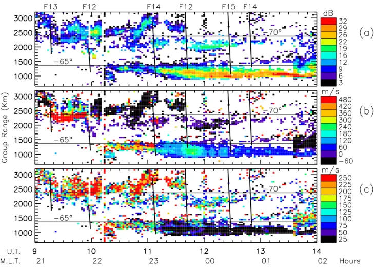
Figure 3 shows range-time-intensity (RTI) plots of (a) the backscatter power (dB), (b) LOS Doppler velocity (m s−1), and (c) Doppler spectral width (m s−1) measured on TIGER beam 15 during 09:00 to 14:00 UT on 27 February 2000. The three parameters were calculated using the standard “FITACF” algorithm (Baker et al., 1995) used to process all SuperDARN autocorrelation measurements. Each pixel rep-resents a parameter estimated using a 7-s integration time re-peated once every two minutes, and sampled at 45-km steps in range. Any echoes FITACF identified as coming from the sea were rejected in this study. The two thin, black horizontal lines in all panels represent magnetic latitudes
Fig. 3. RTI plots of (a) TIGER backscatter power (dB), (b) LOS Doppler velocity (m s−1), and (c) spectral width (m s−1) measured every 2 min on the eastward-looking beam 15 during 09:00 to 14:00 UT on 27 February 2000. Note the colour scale for LOS Doppler velocity is shifted towards large approaching values (i.e. strong azimuthal flows toward the west). The two thin, black, horizontal lines in all panels correspond to magnetic latitudes of −65◦(MQI) and −70◦3. The six diagonal line segments in all panels represent the location of the discrete and diffuse auroral ovals identified along “nearby” transits (see text) of the DMSP F12, F13, F14, and F15 satellites, as labelled. The abscissas have tick marks at 10-min intervals of UT, but nominal values of MLT above MQI are also given.
of −65◦3(MQI) and −70◦3, calculated using altitude ad-justed corrected geomagnetic coordinates (AACGM) (Baker and Wing, 1989).
Beam 15 is the most eastward and magnetic zonal-looking beam of the TIGER radar, reaching a maximum poleward lat-itude of −71.8◦3(range cell 68) before folding back towards
the equator beyond this range (Fig. 1). Magnetic latitude increases steadily at the closest ranges, but at the furthest ranges it increases asymptotically toward −71.8◦3. Beam 15 also traverses a substantial range of magnetic longitude. The nominal MLTs quoted here are for MQI, located nearby the range cells where many of the interesting ionospheric echoes were observed. Beam 15 observations were chosen for display because they provide the most detailed profile of the subauroral ionosphere imaged by TIGER, while also be-ing especially sensitive to zonal flows confined within narrow channels. They are also the best observations for comparison with MQI ground-based measurements.
The DMSP series of spacecraft are near polar
orbit-ing, Sun-synchronous satellites. They have an altitude of 830 km and an orbital period of 101 min. The SS J/4 de-tectors (Hardy et al., 1984) measure precipitating ions and electrons from which spectra of differential energy flux (eV cm−2s−1ster−1eV−1) are calculated every second. The spectra span the energy range 30 eV to 30 keV. The mag-netic coordinates of the satellite track are calculated using Tsyganenko’s (1990) magnetic field lines (see Tsyganenko and Stern, 1996, and references therein) passing through the satellite down to an ionospheric footprint at an altitude 110 km. The difference in magnetic latitudes of points lo-cated at altitudes of 110 km and 300 km are usually <0.1◦ for TIGER observation cells. In this paper we make use of nightside auroral oval boundaries automatically identified in DMSP energy spectra using the logical criteria outlined by Newell et al. (1996).
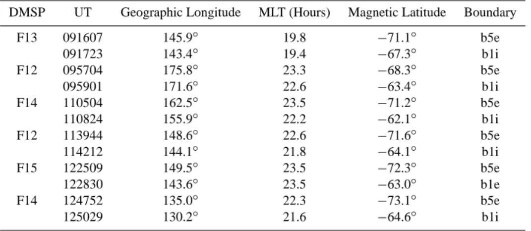
Table 1 is a summary of automatically identified bound-aries specifying the latitudinal extent of the diffuse and dis-crete auroral oval in the nightside ionosphere. The
corre-Table 1. Nightside auroral oval boundaries superimposed in Figs. 3 and 4
DMSP UT Geographic Longitude MLT (Hours) Magnetic Latitude Boundary
F13 091607 145.9◦ 19.8 −71.1◦ b5e 091723 143.4◦ 19.4 −67.3◦ b1i F12 095704 175.8◦ 23.3 −68.3◦ b5e 095901 171.6◦ 22.6 −63.4◦ b1i F14 110504 162.5◦ 23.5 −71.2◦ b5e 110824 155.9◦ 22.2 −62.1◦ b1i F12 113944 148.6◦ 22.6 −71.6◦ b5e 114212 144.1◦ 21.8 −64.1◦ b1i F15 122509 149.5◦ 23.5 −72.3◦ b5e 122830 143.6◦ 23.5 −63.0◦ b1e F14 124752 135.0◦ 22.3 −73.1◦ b5e 125029 130.2◦ 21.6 −64.6◦ b1i
sponding locations of the auroral oval are superimposed as diagonal, black lines drawn in all panels of Fig. 3. The boundaries were chosen using the most equatorward and poleward ion or electron boundaries available, which tended to be “b1i”, the zero-energy ion boundary at the equatorward edge of the proton aurora, and “b5e”, the abrupt drop in elec-tron precipitation at the poleward edge. The individual dy-namic spectra are not shown for brevity, but it is important to consult them to fully understand the unique particle dynam-ics involved during every transit of the auroral oval.
Unfortunately, the satellite tracks were not always closely aligned with the longitude of TIGER beam 15, nor the lon-gitude of any other beam containing interesting scatter (i.e. ∼140◦ to 155◦ geographic at −65◦3). The first transits of the F12 and F14 spacecraft were ∼1.8 h and ∼0.8 h to the east of the TIGER full scan, respectively. The auroral oval boundaries were probably located 1–2◦ further pole-ward in the TIGER FOV due to the familiar equatorpole-ward ex-pansion of the oval toward midnight. The second transit of the F14 spacecraft was ∼1.0 h to the west, implying that the auroral oval boundaries were located ∼1◦ further equator-ward in the TIGER FOV. The remaining transits were more favourably located. Given the substorms occurring during this evening, zonal perturbations in the auroral oval bound-aries were inevitably larger than the familiar statistical vari-ation with MLT. Nevertheless, the DMSP boundaries can be compared with the TIGER observations, keeping in mind that the discrepancies due to zonal structure were <2◦.
Figure 3a reveals that there was patchy scatter poleward of −66◦3with a moderate signal-to-noise ratio (SNR), mostly
in the range 3 to <20 dB (black to green). This scatter was associated with the auroral oval (thick diagonal lines) and polar cap ionosphere. The location of the latter is implied because the poleward edge of the auroral oval is a reason-able proxy for the open-closed magnetic field line boundary (OCB) (Vampola, 1971; Evans and Stone, 1972). Commenc-ing at 10:12 UT, a persistent band of scatter ∼2◦3wide ap-peared at ∼−64◦3. Initially, the SNR was moderate, mostly <20 dB (black to green), but at about 11:08 UT, the SNR
grew to >20 dB (green), and eventually peaked at ∼40 dB (red) near 13:35 UT. The band of scatter also expanded in width to ∼3◦3during 11:00 UT. The DMSP boundaries
sug-gest that this scatter overlapped the equatorward edge of the auroral oval.
Figure 3b shows the auroral and polar cap scatter located poleward of −66◦3had mostly weak receding LOS Doppler velocity, vLOS (dark blue to black) after ∼09:56 UT. This
meant that the true motion must have had a significant east-ward component (recall beam 15 points toeast-wards the east). Consulting a two-cell convection model of the high-latitude ionosphere, such as the DMSP-based Ionospheric Convec-tion Model (DICM) (Papitashvili and Rich, 2002), suggests that beam 15 should have been nearly orthogonal to flows ex-iting the polar cap and veering toward the east at 10:00 UT. However, the sign of the Doppler shift should have been very sensitive to fluctuations in the flow direction of plasma ex-iting the polar cap in proximity to the Harang discontinuity. The observed Doppler shifts were basically consistent with the expected convection velocities.
Figure 3b also shows that during 09:15 to 09:56 UT at ∼−69◦3, there was a burst in vLOS toward the radar at
∼500 m s−1(red). This flow burst immediately preceded the positive deflection in the MQI geomagnetic X component (Fig. 2e), marking the onset of Substorm 1. The flow burst may have been a DP 2 current signature occurring simultane-ously with the 8-nT southward turning of Bz (i.e. driven by
dayside reconnection). Alternatively, it may have been the signature of weak nightside reconnection preceding the sub-storm (e.g. see Watanabe et al., 1998). Did the latter relieve the accumulation of open flux in the magnetotail, and help to explain the absence of a clear growth-phase signature in the MQI magnetometer observations?
Figure 3b also shows that an AWFC occurred during 10:12 to 11:08 UT. The persistent band of scatter at ∼−64◦3had large approaching LOS Doppler velocities up to 500 m s−1 (blue to red). Since beam 15 points more toward the pole than the east at these closer ranges, vLOS ≈ 500 m s−1 implies
small-scale dynamics inaccessible using the existing radar gain, angular and temporal resolution. At 11:08 UT there was a step-like decrease in vLOSto ∼100 m s−1(blue)
approach-ing the radar. Though perhaps a coincidence, the step-like decrease in vLOSwas coincident with another Bzsouthward
turning. Figure 3a also shows a transition to larger power at 11:08 UT. The lower velocities in the flow channel persisted until the end of the record.
Figure 3c shows that during 09:00 to 11:40 UT, the spec-tral widths located in the polar cap ionosphere were generally large (>200 m s−1; red), whereas the sparse scatter associ-ated with the discrete and diffuse auroral ovals had moderate spectral widths (50–150 m s−1; blue and green). Neverthe-less, there was a reasonably sharp transition to large spectral widths at the poleward edge of the auroral oval (the OCB), during this disturbed interval. Although some large spec-tral widths were observed equatorward of the OCB during 27 February, these data suggest the nightside spectral width boundary was a proxy for the OCB (see Parkinson et al., 2002).
Figure 3c also shows that during 10:12 to 11:08 UT, the persistent band of scatter at ∼−64◦3had moderate to large spectral widths (100–250 m s−1; blue to red). As will be shown later, the initial 10-min interval of large spectral widths (>200 m s−1) may have been associated with a fa-miliar burst of Pi2 wave activity occurring at substorm onset (Saito, 1969). Andr´e et al. (1999, 2000) have argued that en-hanced spectral widths observed by SuperDARN radars can be explained by the Doppler spread driven by Pc1–2 hydro-dynamic wave activity. Perhaps broad-band ULF waves re-sponsible for the large spectral widths are largely confined to the polar cap ionosphere during geomagnetically quiet condi-tions, whereas related waves are excited on closed field lines during disturbed intervals.
At 11:08 UT there was a step-like decrease in the spec-tral widths to values <60 m s−1(dark blue and black) which persisted until the end of the record. During this interval, there was vague evidence for ∼20 min quasi-periodic varia-tions in the spectral widths (and perhaps LOS Doppler veloc-ities), barely discernible at the resolution of the radar mea-surements. If real, these perturbations may have been sig-natures of long-period MHD field-line resonances propagat-ing on closed field lines (Samson et al., 1996), or less likely, weak polarisation electric fields carried by atmospheric grav-ity waves generated by the AWFC.
Echoes with low spectral widths have been variously asso-ciated with the main ionospheric trough (Ruohoniemi et al., 1988), the diffuse auroral oval (Jayachandran et al., 2000; Uspensky et al., 2001), and the discrete and diffuse auroral oval (Parkinson et al., 2002). In this particular case, the band of scatter with low spectral widths overlapped the equator-ward edge of the diffuse auroral oval. The latter corresponds to the field-aligned poleward wall of the main ionospheric
So far we have concentrated on observations made using the most eastward looking beam 15. They revealed a nar-row flow channel with vLOS approaching up to 500 m s−1at
∼−64◦3. However, the equivalent RTI plots for the western most beam 0 (and others not shown) revealed a narrow flow channel with vLOS receding up to 450 m s−1 at ∼−67◦3.
The associated scatter also had moderate spectral widths (50– 150 m s−1), but appeared at 09:56 UT, coincident with the start of an impulsive increase in the X component measured by the MQI magnetometer. Clearly, it seems reasonable to surmise these observations were of the same AWFC extend-ing across the radar FOV, with observable irregularities ap-pearing 16-min earlier on beam 0 than beam 15 (09:56 UT vs. 10:12 UT).
It may seem surprising that the PJ/SAID was centred on ∼−64◦3 on beam 15 (east), yet on ∼−67◦3on beam 0 (west). As Fig. 1 shows, magnetic L-shells in the TIGER FOV are inclined by 2◦toward lower geographic latitude in the west. This meant that the AWFC was actually aligned to within ∼1◦of the geographical zonal direction. However, we attach no physical meaning to this because the AWFC probably overlapped the equatorward boundary of the auro-ral oval, a feature statistically located at lower magnetic lat-itude toward the east in the pre-midnight sector. Hence, the geographic zonal alignment was a coincidence.
In summary, an analysis of RTI plots shows that an AWFC occurred during 09:56 to 11:08 UT. Scatter associated with the AWFC appeared on beam 0 at 09:56 UT, but not on beam 15 until 10:12 UT. However, the dynamics of the event were very well defined on beam 15. The observations of vLOSimply there was a narrow jet (∼2◦3) of westward drift
>1 km s−1with longitudinal extent >20◦. The AWFC must have had an extent of at least 1.3 h in MLT. The DMSP ob-servations suggest the AWFC overlapped the equatorward edge of the diffuse auroral oval, a feature normally aligned with the poleward wall of the main ionospheric trough in the evening sector. The end of the event was marked by a step-like increase in backscatter power, and a step-step-like decrease in vLOS and spectral width. Unfortunately, other radars in
the SuperDARN network were either not working, or they recorded sparse scatter, or were too far away in MLT, to fur-ther characterise the event.
3.5 Standard beam-swinging analysis
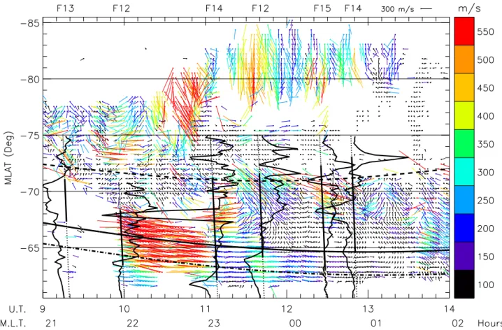
Figure 4 shows two-dimensional flow vectors estimated along TIGER beam 4, the magnetic meridian pointing beam, using the vLOS values measured on all radar beams, and
the beam-swinging technique described by Ruohoniemi et al. (1989). The flow speeds have been colour-coded us-ing intervals of 50 m s−1, and the results for Substorm 2 are not shown because there was no evidence for an AWFC oc-curring then. The beam-swinging technique assumes fairly
Fig. 4. Two-dimensional flow vectors estimated along TIGER beam 4 using the beam-swinging technique at 2-min time resolution during 09:00 to 14:00 UT on 27 February 2000. The solid dots correspond to the time and latitude of the velocity estimate, and the flows were in the direction of the lines leaving the dots. Flows directed toward the right were eastward, and toward the bottom, equatorward. The flow speeds were colour-coded from <125 m s−1(black) to >525 m s−1(red), and the linear scale for an eastward flow of 300 m s−1is shown at top right. As in Fig. 3, the six bold diagonal line segments represent the location of the auroral oval identified along nearby transits of the DMSP satellites. The fluctuating black curves represent the DMSP ion drift measurements made transverse to the satellite tracks (west to the left). As in Fig. 1, Starkov’s (1994) model auroral oval boundaries have been superimposed.
laminar flows with uniform velocity along magnetic L-shells (Freeman et al., 1991), and the distribution of vLOS in the
full scans was usually consistent with this assumption. How-ever, many of the velocity fluctuations are probably artifacts caused by an inability of the technique to reproduce small-scale and short-lived features. Nevertheless, the major trends are representative of the actual flows.
The same DMSP identifications of the auroral oval super-imposed in Fig. 3 have been supersuper-imposed in Fig. 4 (diag-onal black lines). DMSP ion drift measurements of the ve-locity component transverse to the orbital trajectories have also been superimposed, with speed proportional to the dis-tance from the orbital trajectories. Lastly, the auroral oval boundaries (black) given by the Starkov (1994) model are also included for reference, namely the poleward boundary of discrete aurora (dashed curve), the equatorward boundary of discrete aurora (solid curve), and the equatorward bound-ary of diffuse aurora (dashed-dotted curve).
Figure 4 shows that during 11:15 to 13:25 UT, the po-lar cap flows poleward of −77◦3were persistently toward the equator, having speeds of ∼300 m s−1and more. These
were familiar antisunward (but slightly duskward) flows oc-curring in the cross polar cap jet during Bz weakly
nega-tive, but sometimes positive conditions. They may represent flow bursts directly driven by day- or night-side reconnec-tion, and were delayed until the substorm recovery phase (Fox et al., 1999). At lower latitudes, and other times, the polar cap flows were very erratic, and probably poorly deter-mined. However, they had a strong bias toward the equator, and a very weak bias toward the west. A strong equatorward flow burst to speeds of ∼1 km s−1occurred during 10:35 to 10:55 UT and between−75◦3and −81◦3. This flow burst commenced on open field lines during the expansion phase of Substorm 1 (Fig. 2e). Beyond 11:20 UT, the flows in the auroral ionosphere (∼−65◦to −71◦3) were still toward the equator, but they developed a strong eastward compo-nent. This suggests that beam 4 passed through a radar ana-log of the Harang discontinuity, a feature clearly seen near 11:45 UT at ∼−68◦3.
Figure 4 also reveals that the AWFC overlapped the au-roral and subauau-roral ionosphere. During 09:56 to 11:08 UT, very large (>1 km s−1) westward drifts centred on ∼−65◦3
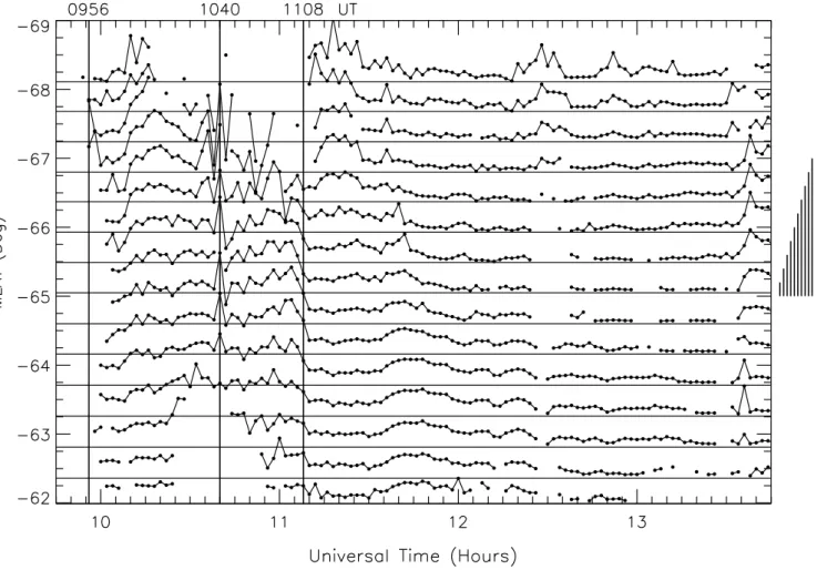
Fig. 5. Stack plot of flow speeds estimated along TIGER beam 4 using the beam-swinging technique at 2-min time resolution during 09:45 to 13:45 UT on 27 February 2000. The flow speeds were calculated at intervals of just under 0.5◦3, and the scale used was 1 km s−1per 1◦3. The ascending scale at right shows speeds of 200, 400,..., 2000 m s−1.
and to the west of the Harang discontinuity occurred con-currently with Substorm 1. Another short-lived burst of westward flow occurred during 11:10 to 11:25 UT between −67◦3and −71◦3, possibly the same substorm signature described by S´anchez et al. (1996). The drifts beyond 11:08 UT and equatorward of −65◦3 were mostly in the range 50–300 m s−1, and predominately westward until the start of Substorm 2 toward the end of the record.
The DMSP ion-drift measurements (black) were in rea-sonable agreement with the zonal velocity components mea-sured by TIGER, when allowing for the location of the satel-lite trajectories relative to the radar FOV. DMSP ion-drift measurements poleward of −75◦3are not shown in Fig. 4,
because the trajectories rapidly traversed many degrees of longitude. The ion-drift measurements made during the first pass of the F13 spacecraft were toward the west, consistent with normal return sunward flows in the dusk sector near 19:50 MLT. During the first pass of the F12 spacecraft at 09:58 UT, the auroral flows were predominately eastward, as might be expected east of the Harang discontinuity (recall the pass was to the east of the radar FOV).
During the first pass of the F14 spacecraft at 11:06 UT, a
narrow ∼1◦westward flow burst with peak speed 3.1 km s−1 was detected at 22:49 MLT and −68◦3. There was also a vertical upward velocity spike of 1 km s−1 (i.e. ion heat-ing). As previously described, the same event was measured just to the east shortly afterward by TIGER, though with a much lower speed. The DMSP spectra show this event was spatially coincident with a flux depletion region (FDR) in-side boundary plasma sheet precipitation, as described by S´anchez et al. (1996). Enhanced westward drifts occur on closed field lines in FDRs (see Fig. 4 of S´anchez et al., 1996), and convection reversals and arc intensifications at their pole-ward edges. Lastly, enhanced westpole-ward drifts correspond to eastward electrojets, which can be mistaken for the recov-ery phase of substorms. Hence, the present event may only appear to have occurred at the end of recovery phase of Sub-storm 1.
Ion-drift measurements made during the other three satel-lite passes were basically consistent with the eastward auro-ral flows and slower westward subauroauro-ral flows observed by TIGER (i.e. the flow reversal boundary).
It is difficult to judge when variations of flow speed oc-curred during and after the AWFC using the results shown in
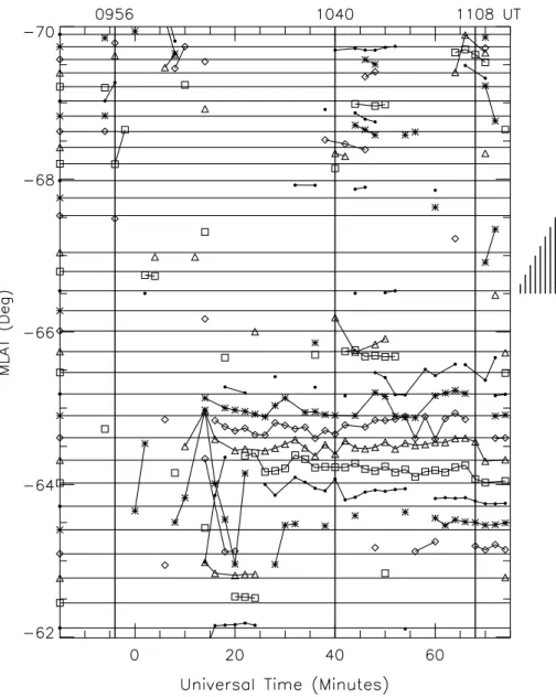
Fig. 6a. Refined beam-swinging analysis (see text) using the LOS Doppler velocities recorded on beam 15 (east). Alternating symbols were used for velocities calculated at different magnetic latitudes and are identified by the symbol superimposed on the left ordinate at the corresponding latitude (e.g. open squares represent velocities at −64◦3). The scale used was 4 km s−1per 1◦3, and the ascending scale at right shows speeds of 500, 1000,..., 4000 m s−1. The time base is in minutes, commencing at 10:00 UT, and the abscissa has tick marks at 5-min intervals of UT.
Fig. 4. Hence, Fig. 5 is an expanded view of flow speeds oc-curring at subauroral latitudes only. The flow speeds were calculated at the maximum time resolution of 2 min, cor-responding to the time separating full scans. The speeds are shown in stack plot form using a scale of 1 km s−1 per
1◦3. An ascending scale of vectors of length 200, 400,...,
2000 m s−1 is shown at right. Using v = E × B/B2, these speeds correspond to electric fields of strength ∼11.9, 23.7,..., 118.7 mV m−1inside the TIGER FOV.
At 09:56 UT, the nominal start of the AWFC, the flow speeds were probably no more than ∼250 m s−1. The speeds were larger at higher latitudes, rapidly increasing to ∼600 m s−1 by 10:12 UT. The speeds continued to grow, peaking to nearly 900 m s−1 by 10:18 UT. A velocity spike
of ∼1.3 km s−1 (77 mV m−1) occurred at 10:40 UT, mark-ing the maximum flow speeds estimated usmark-ing this partic-ular analysis. Using a nominal half-width of ∼100 km for the flow channel (to be justified), this corresponds to a peak electric potential >7.7 kV. At 11:04 UT, the flow speed was ∼800 m s−1, but rapidly declined to ∼200 m s−1 by 11:10 UT, the nominal end of the AWFC. The region of high speed was broader in latitude at the start of the AWFC, and its location decreased in latitude by ∼2◦3towards its end.
At 11:18 UT, the flow speed again peaked to ∼1 km s−1 during the other short-lived flow burst near −68◦3. At 11:42 UT, the low-latitude flow speeds also peaked again, but only to ∼400 m s−1near −64◦3. Perhaps this peak was associated with the lesser auroral intensification to −83 nT
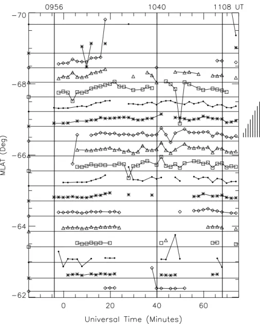
Fig. 6b. The same as Fig. 6a except for beam 0 (west).
beginning near 11:28 UT (Fig. 2e). Thereafter, the subauro-ral flows steadily decayed, reaching values <50 m s−1during 13:00 UT.
Consulting the DICM model suggests that prior to 10:30 UT, there should have been westward flows up to 400 m s−1 equatorward of −65◦3. However, after passing
through the Harang discontinuity at 11:55 UT, the subauroral flows should have rotated toward the east. Clearly, the west-ward flows observed during the AWFC were much larger than typical convection speeds for this sector, and the sub-sequent subauroral flows were in the opposite direction to those normally observed past the Harang discontinuity. The persistence of the AWFC on closed magnetic field lines is inconsistent with nightside reconnection as a driver for the event.
3.6 Refined beam-swinging analysis
The standard beam-swinging analysis applied in the pre-ceding section assumed uniform velocity along magnetic L-shells (Ruohoniemi et al., 1989). However, from an examina-tion of beam 15 observaexamina-tions (Fig. 3), and equivalent obser-vations for beam 0, we know that the AWFC was a very nar-row feature on beam 15 (∼1◦3), somewhat broader on beam 0 (∼2◦3), and aligned in the geographic zonal direction. The DMSP ion drift measurements also suggest the standard beam-swinging analysis (Fig. 4) underestimated the magni-tude of the westward drifts, smearing them over a greater range of magnetic latitude. Hence, we applied the follow-ing simpler beam-swfollow-ingfollow-ing analysis to further scrutinise the LOS Doppler shifts. The geographic westward drift, vw, in
veloc-ity, vLOSusing the following equation:
vw i,j =(vLOS i,j− −veq)/sin(θi−ϕ), (1)
where i varies over all 16 beams, and j over all ranges with ionospheric scatter. θi is the angle between the geographic
meridian and the beam direction, i (e.g. 24.3◦for beam 15), ϕ ≈ 1◦ is a correction equal to the difference between the orientation of the flow channel and the geographic east-west direction, and veq ≈80 m s−1is an estimate of the
equator-ward migration of the flow channel, as revealed in Fig. 4. As θi −ϕ approaches 0◦for beams 7 and 8, vw becomes very
large and changes asymmetrically for even small errors in veq and ϕ. Hence, reasonable estimates of veq and ϕ were
obtained by suppressing the discontinuity in vw centred on
the imaginary beam half-way between beams 7 and 8, and pointing perpendicular to the flow channel.
Figure 6a shows a stack plot of beam 15 results calculated using Eq. (1). The main part of the AWFC was centred near 64.5◦3. It was ∼1◦3wide, and vw was often ∼1 km s−1.
However, during 10:00 to 10:22 UT at ∼63◦3, there is some evidence for unusually large and temporally structured west-ward flows, perhaps peaking to ∼6 km s−1at 10:14 UT. Note that we have excluded all points for which the relative error in vLOS was greater than 50%, and some of the unusually
large velocities persist when applying even more stringent criteria. However, some of the large velocities are artifacts caused by real, meridional ionospheric flow components per-pendicular to the flow channel. These velocity components greatly amplify vw, especially for small θi −ϕ. Lastly,
be-cause of the subsequent absence of backscatter at the equa-torward edge, we cannot tell whether unusually large veloc-ities were present beyond ∼10:30 UT. In light of this analy-sis, and the 3.1 km s−1velocity spike measured by the F14 spacecraft, we speculate that there were larger, more struc-tured flows than portrayed in Fig. 4.
Figure 6b is the results of the same analysis applied to the same time and range windows, but for the western most beam 0. The main part of the AWFC was centred near 67◦3. It was ∼2.5◦wide, and vwwas often ∼1 km s−1. Again, some
of the unusually large values of vwmay have been caused by
real ionospheric flows perpendicular to the flow channel. It is interesting that the velocity spike at 10:40 UT in Fig. 4 was caused by large Doppler shifts on the beams nearly bisecting the radar FOV. Combined, this suggests that there may have been a lot of structure associated with the AWFC that can-not be resolved without using a high resolution, dual radar system.
Clearly, the signatures of the AWFC were narrower, and possibly more structured closer to the Harang discontinuity (Fig. 6a), and became broader at earlier MLT (Fig. 6b). The velocities were largest on the eastern-most beams, and were probably underestimated using the standard analysis, Fig. 4. Lastly, beam 15 results for 11:30 to 12:05 UT obtained us-ing the same analysis (not shown) show a westward velocity enhancemnet to ∼700 m s−1, propagating equatorward from ∼66◦3to 62◦3at a similar velocity (c.f. Fig. 5). The event
was initiated at the onset of the lesser intensification follow-ing Substorm 1 (Fig. 2e). We speculate that the associated current surge launched an atmospheric gravity wave which carried a meridional polarisation field.
3.7 Other ground-based observations
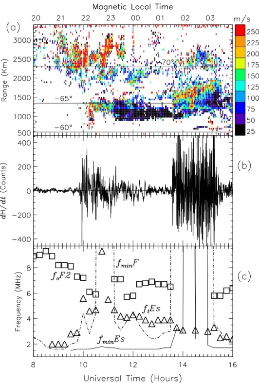
Figure 7a shows a range-time-intensity (RTI) plot of the Doppler spectral width (m s−1) measured on TIGER beam 15 during 08:00 to 16:00 UT on 27 February 2000. A shorter interval of this data was shown in Fig. 3c, but is shown again for comparison with (b), the induction coil magnetogram showing ultra-low frequency (ULF) wave activity recorded nearby at MQI, and (c) the various critical frequency pa-rameters scaled from MQI routine ionograms recorded ev-ery 15 min. MQI (−65◦3) has the same magnetic latitude as range cell 26 (1350 km) of beam 15, located 406 km away. However, it is meaningful to compare observations made at these two locations, even though the detailed ionospheric electrodynamics must be different.
Figure 7a shows there was a burst of large spectral widths (>200 m s−1) during 10:06 to 10:12 UT at latitude −62◦
to −64◦3. This was followed by an interval of moderate
spectral widths (150–200 m s−1) at ∼−64◦3during 10:08 to 11:12 UT (the AWFC). The next major episode of auro-ral scatter with large spectauro-ral widths (>150 m s−1) suddenly commenced at 13:36 UT, coincident with the onset of Sub-storm 2 (c.f. Fig. 2e).
An initial qualitative comparison suggests the variations in spectral width at ∼−65◦3(Fig. 7a) were roughly coincident with the variations in ULF wave activity recorded at MQI (Fig. 7b). A dynamic power spectrogram of the MQI magne-tometer response (not shown) confirms that there were two major episodes of ULF wave activity coincident with Sub-storms 1 and 2. When allowing for spatial integration across the large, effective FOV of the ground-based magnetometer (∼300 km) (Ponomarenko et al., 2001), and its spatial sepa-ration from beam 15, the agreement between the two kinds of data is reasonable. This suggests that the spectral width en-hancements were related to bursts of broad-band ULF wave activity, and not small-scale convective turbulence (i.e. if such a distinction exists).
DMSP spacecraft data confirm that the many kinds of ULF wave activity shown in Fig. 7b occurred on closed field lines in the auroral oval. A detailed analysis of the different kinds of wave activity is beyond the scope of this study. How-ever, Figure 7b shows that there was a burst of Pi2 waves (40–150 s) near the start of Substorm 1, ∼09:50 UT, and Pi1 (1–40 s) waves quickly developed (PiB evolving into PiC), becoming most intense during 10:45 to 11:05 UT. Pi3 (5– 40 min) (or Ps6) waves were present throughout the event and are clearly evident during the recovery phase up until 12:32 UT (Fig. 7b). Concurrent signatures of Pi3 wave activ-ity were also apparent in the radar measurements (Figs. 3 and 7a). Figure 7b also shows that there was a burst of Pi2 waves near the start of Substorm 2, 13:33 UT, and a 2-h episode of intense Pi1, Pi2, and Pi3 wave activity
fol-Fig. 7. (a) RTI plot of Doppler spectral width (m s−1) recorded every 2 min on TIGER beam 15 during 08:00 to 16:00 UT on 27 February 2000. (b) The time derivative of the geomagnetic H component measured at 1-s intervals by an induction coil magnetometer located at MQI. (c) The critical frequency parameters fminEs(continuous line), fminF(dash-dot-dash line), ftEs(open triangles), and foF2 (open squares),
all scaled from routine ionograms recorded at 15-min intervals by an analogue ionosonde located at MQI. The abscissas have tick marks at 10-min intervals of UT, and nominal values of MLT at MQI are shown at top.
lowed shortly thereafter, lasting until near the end of recov-ery phase, ∼15:33 UT.
The frequency parameters shown in Fig. 7c include a mea-sure of ionospheric absorption, fminEs (continuous line), a
measure of ionospheric absorption and blanketing Es, fminF
(dash-dot-dash line), the top frequency of auroral Es traces, ftEs (open triangles), and foF2 (open squares). The
be-haviour of these parameters revealed two major absorption events, the first occurring during 10:30 to 11:15 UT (i.e. Sub-storm 1), and the second occurring during 13:30 to 15:15 UT
(i.e. Substorm 2). The times of major absorption were de-fined by increases in the parameter fminF to at least beyond
the parameter foF2. However, it is possible that the F-region traces were lost because ion-neutral friction heating resulted in the loss of F-region ionisation.
The parameter foF2 was depressed during Substorm 1, perhaps due to an enhanced recombination rate associated with the AWFC located just equatorward of MQI. The ma-jor absorption event during Substorm 1 was preceded by an episode of auroral Es with ftEs, increasing to 5.6 MHz
at 10:00 UT, near the substorm onset. At 10:45 UT, ftEs
reached a maximum value of 9.3 MHz, close to the peak expansion phase and the largest, smoothed velocities in the AWFC. Absorption during Substorm 2 was even more in-tense, resulting in the loss of auroral Es traces as well as F-region traces. We attribute these absorption events to en-ergetic particle precipitation intensifying in the auroral oval located above MQI, just poleward of the AWFC. Note that nearly continuous ionospheric scatter was recorded by the oblique looking TIGER radar during these absorption events. An analysis of coincident vertical TEC measurements (not shown) made using ground-based receivers located at MQI and Hobart also suggest that the auroral oval was located above, or nearby, MQI during the study period. Observations made under a broad range of geomagnetic conditions suggest that the centre of the main ionospheric trough was probably located ∼2–5◦further equatorward during 27 February. This
is consistent with alignment of the AWFC with the poleward edge of the trough, and overlapping the equatorward edge of the diffuse auroral oval.
4 Discussion and conclusions
An AWFC resembling a PJ/SAID occurred simultaneously with Substorm 1 on 27 February 2000. We summarise the observed sequence of events, and provide plausible explana-tions for their meaning as follows.
Variations in the geomagnetic X component measured at MQI (−65◦3) showed manifestation of Substorm 1 occur-ring in the evening sector (∼22:00–23:00 MLT) duoccur-ring 09:58 to 11:10 UT. This substorm may have been triggered by a weak Bznorthward turning, following a succession of deeper
Bz southward turnings to less than −4 nT. Surprisingly, the
geomagnetic X and Y components at MQI showed no obvi-ous growth-phase signatures; rather the onset of Substorm 1 was preceded by a ∼60-nT northward impulse in the X com-ponent, peaking at 09:58 UT. The impulse was coincident with the start of a dispersionless particle injection observed by the LAN-L 1989-046 geosynchronous spacecraft located at 6.6 RE and 22:53 MLT. The geomagnetic X component
subsequently swung deeply negative, indicative of substorm onset. Recovery phase commenced at 10:53 UT, and the sub-storm finished at 11:10 UT.
Why was there no clear growth phase signature in the MQI geomagnetic X component preceding the onset of Substorm 1? At this time MQI was located at 21:00 MLT, perhaps too
far to the east to detect the gradual growth of the DP 2 east-ward electrojet, yet too far to the west to detect the grad-ual growth of the DP 2 westward electrojet. However, con-sider an alternative possibility. The growth phase signature of Substorm 1 may have been masked by the effects of the AWFC. Near the start of Substorm 1, 09:53 to 10:02 UT, there was a positive deflection in the X component, consis-tent with an AWFC driving an eastward Hall current. Ion-neutral friction must have rapidly elevated the F-region re-combination rate, reducing the ionospheric electron density, and thus ionospheric conductivity. Hence, beyond 09:58 UT, the effect of the eastward Hall current on the magnetome-ter began to diminish, whereas the effects of the westward electrojet rapidly increased. By 10:02 UT, the latter began to have a greater effect on the magnetometer than the eastward Hall current driven by the AWFC.
The MQI Z-component variations were opposite in sign to the X-component variations during the intervals dominated by eastward Hall and westward electrojet currents. They imply these currents were centred just poleward of MQI where the ionospheric conductivity was larger deeper into the auroral oval. The beam-swinging vectors may have been poorly determined just poleward of the AWFC, but Fig. 4 shows there was evidence for strong eastward and equator-ward flows during 10:20 to 11:00 UT between −67.5◦ and −71.5◦3. Moreover, ion-drift measurements made during the first passes of the F12 and F14 spacecraft also showed strong eastward flows closer to midnight just poleward of the AWFC. Combined with conductivity enhancements, these eastward flows are consistent with the familiar −X deflec-tions observed at MQI.
Figure 3 showed TIGER observed signatures of an AWFC in the backscatter power, LOS Doppler velocity, and Doppler spectral width, simultaneous with the MQI magnetometer signatures of the current wedge forming during Substorm 1. Although scatter associated with the AWFC was not ob-served on the eastern-most beam 15 until 10:12 UT, it was observed earlier at 09:56 UT on the western-most beam 0. On beam 15, the scatter was ∼2◦3wide, centred on −64◦3, and vLOS was up to 500 m s−1 towards the radar. On beam
0, the scatter was centred on −67◦3, and vLOS was up to
450 m s−1away from the radar. The largest values of vLOS
were confined to a very narrow channel <1◦3wide. These observations implied very large westward drifts (>1 km s−1) aligned parallel to the equatorward edge of the auroral oval. DMSP measurements of precipitating particles confirmed the narrow flow channel probably overlapped the equatorward edge of the diffuse auroral oval. MQI ionosonde and TEC measurements also helped to validate this interpretation.
Figure 3 showed that for ∼2 h beyond the end of the AWFC, there was a channel of scatter with low spectral widths resembling the scatter normally associated with the main ionospheric trough (Ruohoniemi et al., 1988). The irregularities were also slowly drifting toward the west at ∼100 m s−1 in a region located to the east of the Harang discontinuity, whereas statistical convection models indicate eastward flows dominate this region. It seems reasonable to
ral regime found equatorward of the influence of magneto-spheric convection (i.e. the flow reversal boundary). The main ionospheric trough and the plasmapause were proba-bly located in proximity to this band of scatter (∼−63◦3on beam 15).
The analysis of full-scan results, Fig. 5, revealed that the magnitude of flows in the AWFC must have grown during the 22-min interval, 09:56 to 10:18 UT. There was an especially sharp rising edge at 10:08 UT near the poleward extremity of the AWFC, coincident with a peak in the flux of hot protons measured by the LAN-L 1989-046 spacecraft. Peak flows occurred at 10:40 UT, coincident with a step-like decrease in the flux of hot protons at 10:40 UT. However, the more refined analysis of Doppler shifts, Figs. 6a and b, revealed there were poorly resolved, small-scale motions during the event, with evidence for speeds >4 km s−1at substorm onset near the equatorward edge of the AWFC. The AWFC mi-grated toward lower latitude at ∼80 m s−1, and there was a slight tendency for the width of the flow channel to con-verge in latitude with time. At the end of the recovery phase, the flows decayed rapidly during the 6-min interval 11:04 to 11:10 UT. The subsequent westward flows, probably as-sociated with the main trough, trended toward lower values during the following two-hour interval. The life time of the main part of the AWFC was 74 min (09:56 to 11:10 UT).
Interestingly, the DMSP F14 spacecraft measured a 3.1 km s−1 westward flow burst at the end of the recovery phase, 11:06 UT. This flow burst was located well inside the discrete auroral oval, a region thought to map to closed field lines. Hence, this event was probably not directly driven by nightside reconnection, and may constitute a short-lived AWFC. Its behaviour was similar to that of the large west-ward flows coincident with flux depletion regions (FDRs) oc-curring in the boundary plasma sheet (S´anchez et al., 1996). The AWFC observed during 09:56 to 11:10 UT had much in common with the observed characteristics of PJ/SAIDs, and the theoretical expectations of Anderson et al. (1993) and De Keyser (1999). For example, the AWFC was broader in latitude toward earlier MLT, and had a slight tendency to converge with time (Anderson et al., 1993). The gradual equatorward movement of the flow channel at ∼80 m s−1is consistent with the earthward migration of a hot ion plasma front toward the plasmapause, and the PJ/SAID took at least 22 min to fully develop (De Keyser, 1999). However, un-like earlier satellite observations which show that PJ/SAIDs do not occur until the recovery phase, our event commenced at substorm onset and finished at the end of recovery phase. Does our AWFC only briefly satisfy the Anderson et al. def-inition of a PJ/SAID (i.e. westward drifts >1 km s−1), be-cause the hot plasma front never reaches the plasmapause prior to the end of the recovery phase? The event remained relatively weak and structured, but it might have been the precursor of a true PJ/SAID which never fully developed.
of ∼1 km s−1and latitudinal widths of ∼2–3 . The SARAS shown in Fig. 4 of Freeman et al. (1992) is surprisingly sim-ilar to the AWFC shown in our Fig. 4. SARAS occur in the afternoon sector, and when allowing for westward phase speeds of 1–4 km s−1, the starts of SARAS are probably syn-chronised to substorm onset. Our AWFC was not directly driven by magnetic reconnection, but occurred in the pre-midnight sector, close to the initial hot particle injection near substorm onset. AWFC, SARAS, and PJ/SAIDs may be dif-ferent manifestations of closely related (or the same) electro-dynamic process.
Unlike previous measurements of PJ/SAIDs made using polar orbiting spacecraft, the SuperDARN technique is ca-pable of observing the evolution of related events with good resolution in both space and time. Unfortunately, the AWFC reported here was not observed with other radars in the net-work, including the conjugate Northern Hemisphere radars. This is due to instrument failures, the absence of suitable backscatter, or the inappropriate MLT or latitude of the radars. Thus, we cannot say anything about the conjugacy of the AWFC, nor impose further constraints on any magneto-spheric source. For now, we can only surmise our structured AWFC had a longitudinal extent >20◦, or at least 1.3 h in MLT.
The importance of the ionosphere in generating and reg-ulating the lives of PJ/SAIDs can be understood as follows. First, note the F-region conductivity can be larger than the E-region conductivity in the nightside ionosphere (Du and Stening, 1999). Now consider three ionospheric regions, in-finite in the zonal direction, but with different Pedersen con-ductivities, namely a nightside mid-latitude ionosphere with moderate conductivity, a main ionospheric trough with low conductivity, and an auroral ionosphere with large conductiv-ity. If the magnetosphere imposes the same poleward electric field across these three regions, there will be a divergence of Pedersen current across the two junctions. Positive charge will accumulate in the equatorward wall of the trough, and negative charge in the poleward wall, until ∇ · Jp = 0.
Hence, the poleward electric field will intensify across the trough, and there will be a subsequent increase in westward drift. The associated increase in ion-neutral friction will fur-ther reduce the Pedersen conductivity, and furfur-ther increase the polarisation field, etc. In a sense, the magnetosphere-ionosphere coupling acts like a PJ/SAID generator, draw-ing energy from the magnetosphere via field-aligned cur-rents. However, ionospheric feedback can only partly explain PJ/SAIDs due to their concentration in the evening sector.
This electrodynamic behaviour is similar to that proposed for drifting auroral arcs in which enhanced poleward elec-tric fields are observed in plasma-depleted regions just equa-torward of the arc (Lewis et al., 1994). The divergence of Pedersen current across step-like changes in the iono-spheric conductivity is partly compensated for by the upward