Channel equalization and interference reduction using scrambling and adaptive amplitude modulation

Channel Equalization and Interference

Reduction Using Scrambling and

Adaptive Amplitude Modulation

RLE Technical Report No. 558

June 1990

Adam S. Tom

Research Laboratory of Electronics Massachusetts Institute of Technology

P

Channel Equalization and Interference Reduction

Using Scrambling and Adaptive Amplitude Modulation

by Adam S. Tom Submitted to the

Department of Electrical Engineering and Computer Science

on May 11, 1990 in partial fulfillment of the requirements for the Degree of Doctor of Philosophy in Electrical Engineering

Abstract. In order to appreciate the increased resolution of high-definition images, a

means of reducing the degradation due to channel defects needs to be employed. Conven-tional methods of channel equalization use adaptive filters. These methods require long convergence times, are limited by the length of the filters, and require high computational complexity at the receiver. These are undesirable for television receivers which should be available to the consumer at a resonable cost. In addition, these methods do not reduce additive channel noise, nor do they reduce interference from other signal sources.

Presented in this thesis is a new method of channel equalization, interference reduc-tion, and noise reduction based upon Adaptive Amplitude Modulation and Scrambling. Adaptive Amplitude Modulation is a noise reduction technique, and Scrambling is a scanning method that decorrelates any channel defects and makes them look like ran-dom noise to the desired signal. Also presented is a robust transmission system termed

Adaptively Modulated and Scrambled Pulse Amplitude Modulation (AMSC-PAM) which

incorporates this new channel equalization and interference reduction method.

This new method of channel equalization and interference reduction has several ad-vantages. Unlike conventional equalization schemes, which employ adaptive filters, our equalization and interference-reduction scheme does not require a long convergence time to find the filter coefficients. It only requires simple computations at the receiver and is not limited to a maximum length of the channel impulse response that it can equal-ize. Our scheme can equalize a channel that has an impulse response of any length and does not require transmission of a training sequence. Our equalization and interference reduction method is limited, however, by the power of the channel defects and is more sensitive to mistiming errors than transmission methods that do not use Scrambling.

AMSC-PAM is a robust transmission system that codes a signal so that it can better withstand channel defects and delivers greatly improved images to the receiver with-out having to increase the peak transmission power. AMSC-PAM can make channel degradations of up to a 25dB-CNR power level imperceptible to just perceptible in the demodulated image. In addition, AMSC-PAM can be used in conjunction with conven-tional equalization methods

The Adaptive Amplitude Modulation algorithm is optimized, and its ability to reduce noise is increased over existing methods. Scrambling is discussed, and the motivation behind Scrambling is given. The type of transmission defects that are considered are mistiming errors, additive channel noise, co-channel and adjacent-channel interference, multipath, and frequency distortion. The AMSC-PAM transmission system is described,

and its ability to equalize a channel and to reduce interference and noise at radio fre-quencies (RF) is investigated.

Thesis Supervisor: Dr. William F. Schreiber Title: Professor of Electrical Engineering

To Mom and Dad

Acknowledgments

I would like to thank my advisor Dr. William F. Schreiber for his support and guid-ance. He made my stay at MIT a pleasant one. Not only did he provide technical insights but tried to instill in all of us a social responsibility and awareness that, hopefully, we shall all carry with us in our careers. I would also like to thank my readers Dr. Jae S. Lim and. Dr. Arun N. Netravali for their support and viewpoints.

I am grateful to John Wang, Chong Lee, and Dave Kuo for maintaining our computing and display facilities and to Julien Piot for helpful discussions and suggestions. I would also like to thank Cindy LeBlanc for making everything go smoothly.

Many friends and family have made my stay at MIT enjoyable; I wish to thank them all. Sometimes during one's studies, one can be overwhelmed with the trials of school. It is these people that help one carry on. Thank you.

Contents

1 Introduction 10

2 Adaptive Amplitude Modulation

2.1 Lowest Frequency Component.

2.2 Calculating the Adaptation Factors ... 2.3 Origins of Distortion . . . ....

2.4 Decimation and Interpolation of the Highpass Component

15 ... ...20 . .... .,.. . . 28 ... ...38 ... ...39 ... ...43 ... ...46 ... ...49 . . . ... .. 52 . . . 55

2.5 Subsampling and Distortion Level ... 2.5.1 The Search Method . . . . 2.5.2 The Distortion Measure and Level . 2.5.3 Stills ... 2.5.4 Sequences ... 3 Scrambling 3.1 Picture Coding . . . . 3.2 Channel Defects . . . . 3.3 Examples ... 4 Adaptive Amplitude Modulation and Scrambling 4.1 Why It Works . . . . 4.2 Interaction of Adaptive Amplitude Modulation and 65 65 67 70 74 ... 74 Scrambling... 77

5 Interference Reduction and Channel Equalization

5.1 The Transmission System: AMSC-PAM ...

5.2 Mistiming Errors . ... 5.3 Noise. ...

5.4 Co-Channel Interference ... 5.5 Adjacent-Channel Interference ... 5.6 Multipath and Frequency Distortion ...

86 86 94 96 96 102 106 112 6 Conclusion I O ... ... ... .. . . . . . . . ... ...

List of Figures

2.1 Block diagram of adaptive modulation. ... 18

2.2 Block diagram of adaptive demodulation ... 19

2.3 Visual masking ... 22

2.4 The unit-step response of a two-channel system and the ideal adaptation factors for this signal ... 24

2.5 Overshoot versus prefilter standard deviation. ... 26

2.6 The optimal band-separation Gaussian filter-pair. ... 27

2.7 The original CMAN and GIRL pictures. ... 28

2.8 The highpass response of CMAN and GIRL using the final Gaussian filter-pair ... ... 29

2.9 The highpass and decimated lowpass components of CMAN using an av-eraging prefilter and a linear postfilter. Notice the aliasing. The highpass component has an offset of 128. ... 30

2.10 Evolution of signals in the adaptive modulation process. ... 33

2.11 Highpass component, adaptation factors, and adaptively modulated high-pass component of CMAN. ... ... 35

2.12 Demodulated signals when no adaptive modulation is used and when adap-tive modulation is used when transmitting over a 20dB CNR channel. .. 36

2.13 Histograms of the highpass (a) and adaptively modulated highpass (b) components of CMAN ... 37

2.14 The horizontal frequency axis of the power spectra of the highpass and adaptively modulated highpass components of CMAN. ... 37

2.15 Distortion occurs when the absolute value of the interpolated subsamples is less than the absolute value of the highpass samples. ... 40

2.16 Two different methods of subsampling and interpolation: optimal decimation-and-interpolation and maximum-linear ... 42

2.17 Optimal scaling factor versus CNR ... 44

2.18 Demodulated pictures using the optimal decimation-and-interpolation method of calculating the adaptation factors with a scaling factor of 1.2 under noiseless and noisy (20dB CNR) channel conditions ... 45

2.19 The Secant Method. ... 48

2.20 Plot of block distortion versus decrease in the value of the associated sam-ple of that block for many blocks along a horizontal line. ... 48 2.21 Block diagram of the iterative method of calculating the adaptation factors. 50

2.22 Demodulated pictures, distortion, and histograms of distortion for various

iteration numbers. ... 51

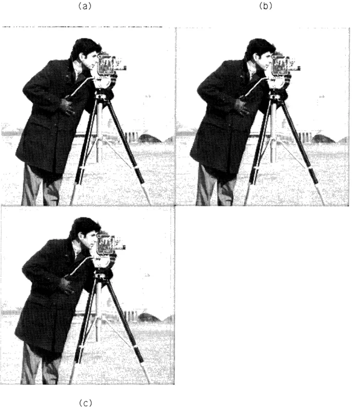
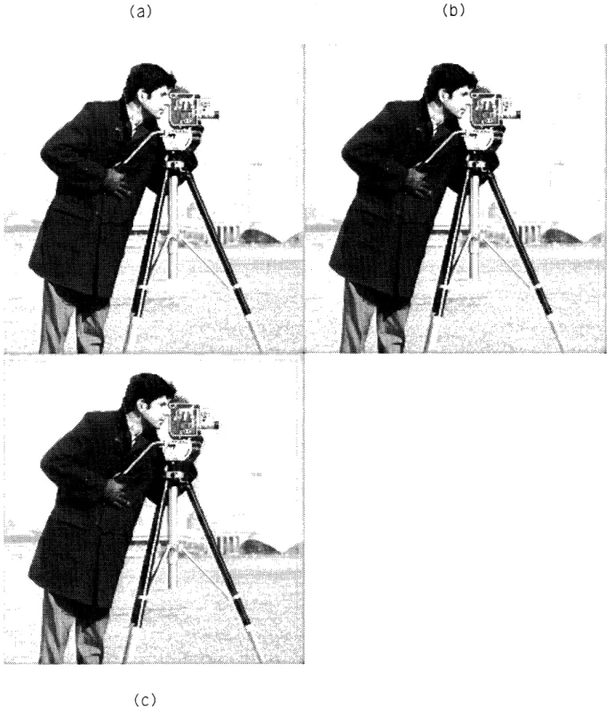
2.23 Demodulated pictures using the root-mean-squared-error distortion mea-sure at three distortion levels: (a) 5%, (b) 15%, and (c) 25% ... 53 2.24 Demodulated pictures using the peak-absolute-error distortion measure at

three distortion levels: (a) 10%, (b) 20%, and (c) 30%. ... 54 2.25 Comparison of three methods of calculating the adaptation factors. .... 56 2.26 One original frame and one noisy frame (20dB CNR) . ... 57 2.27 Using linear interpolation of the maximum absolute values in 4x4x4 blocks

under ideal and noisy (20dB CNR) channel conditions. . ... 58 2.28 Using the iterative method to calculate the adaptation factors in 4x4x4

blocks under ideal and noisy (20dB CNR) channel conditions . ... 59 2.29 Demodulated pictures produced when state is passed from frame to frame

in the iterative method under ideal channel conditions. . ... 61

2.30 Two distortion curves. ... 62

2.31 Results of using the 2-D iterative method on each frame separately under ideal and noisy (20dB CNR) channel conditions . ... 63

3.1 Raster scanning. ... 66

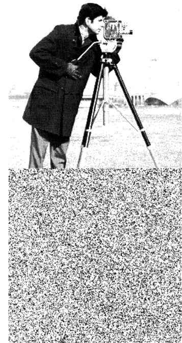
3.2 Block diagram of scrambling. ... 69 3.3 Scrambling of CMAN. The effect of scrambling upon the image and upon

its power-spectrum density. ... 71

3.4 The appearance of 40% multipath without and with scrambling ... 72 3.5 The appearance of 40% interference without and with scrambling .... 72 4.1 Block diagram of adaptive modulation and scrambling at baseband. ... 75 4.2 Root-mean-square value of the adaptively modulated highs versus the

maximum adaptation factor. 78

4.3 The rms value of noise in blank areas versus the maximum adaptation factor. 79 4.4 The rms error over the entire picture versus the maximum adaptation factor. 80 4.5 The demodulated pictures corresponding to a maximum adaptation factor

of (a) 8, (b) 16, (c) 32, and (d) 64, where the picture is degraded by a 40%

echo ... 81

4.6 The demodulated pictures corresponding to a maximum adaptation factor of (a) 8, (b) 16, (c) 32, and (d) 64, where the picture is degraded by an

80% echo. 82

4.7 The rmse of the demodulated signal versus the maximum adaptation factor when white Gaussian noise (20dB CNR) is added in the channel ... 84 4.8 Demodulated pictures for four maximum values of the adaptation factors:

(a) 8, (b) 16, (c) 32, and (d) 64. The channel is degraded by AWGN at a

20dB CNR ... ... 85

5.1 Block diagram of the AMSC-PAM transmission system . ... 87 5.2 Filtering action of the pulse x(t) on the sequence y'[n] ... . 93 5.3 The demodulated pictures for four values of r,/T: (a) 0.05, (b) 0.1, (c)

5.4 A comparison of four demodulated pictures that suffer from mistiming

errors ... 97

5.5 Demodulated pictures at 4 levels of noise: (a) 15dB, (b) 20dB, (c) 25dB,

and (d) 30dB CNR ... 98

5.6 Demodulated picture at a CNR of 25dB. Picture (a) results when no adap-tive modulation is used, and picture (b) results when both adapadap-tive

mod-ulation and scrambling are used ... 99

5.7 Interfering pictures when the offset frequency is: (a) 360 Hz, (b) 604 Hz,

(c) 10010 Hz, and (d) 20020 Hz ... 101

5.8 Interference when an undesired signal has been offset by 10010 Hz and is

at a D/U ratio of 17dB. ... 102

5.9 The evolution of the specturm of (u (t) cos wt) * g(t). . . . ... 103 5.10 The demodulated signal when co-channel interference exists in the channel

using AMSC-PAM for four values of a: (a) 1.0, (b) 0.5, (c) 0.25, and (d)

0.125.10 ... ... ... 1044..

5.11 The appearance of co-channel interference at a 12dB D/U ratio using PAM when (a) neither adaptive modulation nor scrambling is used, (b) only adaptive modulation is used, (c) only scrambling is used, and (d) both are

used . . . 105 5.12 The demodulated signal when adjacent-channel interference exists in the

channel using AMSC-PAM for four values of a: (a) 100, (b) 50, (c) 35,

and (d) 10. ... 107

5.13 The appearance of adjacent-channel interference at a -31dB D/U ratio using PAM when (a) neither adaptive modulation nor scrambling is used, (b) only adaptive modulaton is used, (c) only scrambling is used, and (d)

both are used. . . . ... 108

5.14 The demodulated signal when multipath exists in the channel using AMSC-PAM for four values of a: (a) 0.4, (b) 0.3, (c) 0.2, and (d) 0.15. ... . 110 5.15 The appearance of 20% multipath using PAM when (a) neither adaptive

modulation nor scrambling is used, (b) only adaptive modulation is used, (c) only scrambling is used, and (d) both are used ... 111

6.1 The demodulated image when conventional PAM is used for transmission. 118

6.2 The demodulated image when AMSC-PAM is used for transmission.... 119

Chapter 1

Introduction

In many communications applications, a transmitter sends a desired signal through a nonideal channel, which degrades the signal in some unknown manner, and a receiver

observes this degraded signal. The types of degradation that may occur in the channel are interference from other signal sources, intersymbol interference (including multipath, a nonideal frequency response, and mistiming errors in sampling), and additive noise. Any signal processing technique or algorithm used to reduce intersymbol interference falls under the term channel equalization. Common methods of channel equalization and of reducing additive noise employ the use of adaptive filters [Luc65] [Luc66] [LR67] [Gia78]. Proper bandlimiting, band separation, and in extreme cases, spread-spectrum techniques are examples of methods for reducing interference from other signals [Dix84]. Unfortunately, the causes of intersymbol interference are not stationary, and hence, adaptive filters are necessary to reduce the amount of the resulting degradation. If the channel were stationary, then the channel characteristics would only need to be determined once, and we could fix the filter in each receiver. This would require very little signal processing while the signal was being received because the filter had already been determined. Adaptive filters make an estimate,

i[n],

that minimze a function of the error between the desired signal, i[n], and the estimated

response, lt[n], where the error is,

e[n] = i[n] - ;In](1.1)

Two common algorithms used to calculate the filter coefficients are the Least Mean Squared Error (LMS) and the Recursive Least Squares (RLS) algorithms [Orf85]. Finding the optimal filter which minimizes the mean-squared error requires knowledge of the statistics of the observations and of the error, which we do not have. Solving the optimal filter by means of the RLS algorithm requires inverting an nxn matrix when observation

o[n] is made. In order not to invert directly the matrix, the algorithms do an iterative

search for the filter coefficients.

These two channel equalization schemes calculate the optimal adaptive filter itera-tively either by a gradient search or by recursively finding the inverse of an nxn matrix. Gradient search methods can have a long convergence time that depends upon the spread of the eigenvalues of the autocorrelation matrix of the observation samples, y[n]. The convergence time is an indication of the algorithm's ability to track the nonstationarities of the channel. Methods that invert a matrix have shorter convergence times; however the complexity of the calculations is high. Neither of these methods actually reaches the optimal filter coefficients, but fluctuates about the optimal values. The ability of these methods to equalize the channel is limited by the length of the filter. For example, an adaptive transversal filter of length M cannot equalize an echo that has a delay longer than M samples. In addition, a training sequence must be transmitted periodically as part of the signal in order to facilitate the adaptive filter algorithms.

Described herein is a novel method of channel equalization, noise reduction, and in-terference reduction based upon the ideas of adaptive amplitude modulation and pseudo-random scanning (i.e., scrambling). Adaptive amplitude modulation is a noise-reduction method that advantageously exploits the visual masking phenomenon. Because changes in luminance mask noise in close proximity to the luminance changes, noise is less visible in busy areas than in blank or slowly varying areas of an image. This is a consequence of visual masking. Adaptive amplitude modulation makes use of this property of the

human visual system by adaptively varying the modulation indices of the transmitted video signal in such a manner that noise is significantly reduced in the blank and slowly varying areas of the image and reduced to a lesser extent in the busy areas. The end result is a greatly improved image at the receiver.

Implementation of adaptive amplitude modulation requires that the original input im-age be decomposed into a lowpass and a highpass frequency component. The decimated lowpass signal is sent digitally in some noise-free manner, and the highpass component is adaptively modulated by multiplying it with a time-varying set of modulation indices, or adaptation factors. It is important to note that the signal which has been adaptively modulated has the same peak power as the original signal. The cost of using adaptive amplitude modulation is side information that must be sent to the receiveer; however, the amount of side information is small.

Scrambling is a method of decorrelating channel defects and makes degradations ap-pear as random noise. The idea of scrambling is an extension of the idea behind Roberts' pseudorandom noise technique, or dithering, where quantization noise due to coarse quan-tization is converted to uncorrelated noise, which is less subjectively objectionable than correlated noise. Scrambling is a method of pseudorandomly scanning through an image; thus, the transmitted signal looks like random noise to any other signal. Conversely, after descrambling at the receiver, any other signal (even the transmitted signal's own reflection) looks like random noise to the received, desired signal.

The combination of adaptive amplitude modulation and scrambling equalizes the channel and reduces interference and noise by first adaptively modulating the video signal and then scrambling it at the transmitter. At the receiver, the signal is first unscrambled and then adaptively demodulated. Scrambling converts any intersymbol intersymbol interference, frequency distortion, or interference from other signals into pseudorandom noise, and adaptive amplitude modulation reduces any pseudorandom degradations in the image and additive channel noise. In this manner, interference and noise are reduced, and the channel is equalized. This method requires no convergence time, no complicated mathematical calculations, and no training sequences. In addition, adaptive amplitude modulation and scrambling are not limited by the length of a filter

or the associated fluctuations of the coefficients; adaptive amplitude modulation and scrambling can equalize channels with an impulse response of any duration. The use of adaptive amplitude modulation and scrambling is limited, however, by the power of the resulting noise-like degradation due to scrambling and is sensitive to the synchronization of the sampling at the receiver as are the conventional equalization algorithms.

Because of the recent interest in the efficient transmission of high-definition images or television (HDTV), this research shall use images as the primary source of signal data. This thesis consists of four parts. A basic method of adaptive amplitude modulation exists; however, its ability to reduce noise can be improved. In Chapter 2, we investigate in depth the adaptive amplitude modulation algorithm. In this portion of the research we optimize and improve the performance of the adaptive amplitude modulation algorithm by determining the minimum amount of low-frequency information that we must transmit digitally, investigating different methods of calculating the adaptation factors and of interpolation, and determining the best tradeoff between noise reduction and distortion. In Chapter 3, we describe and give the motivation behind scrambling. In Chapter 4, we explore the interaction of scrambling and adaptive amplitude modulation to determine how much noise reduction should be performed in the presence of scrambling. In Chapter 5, we apply adaptive amplitude modulation and scrambling to reduce interference in and equalize a time-varying channel at radio frequencies. We will look at mistiming errors, additive channel noise, co-channel and adjacent-channel interference, frequency distortion, and multipath. This will entail finding the degree of intersymbol interference and interference from other signals that adaptive amplitude modulation and scrambling can make imperceptible to just perceptible.

Throughout this thesis we have processed 256x256 pictures; however, all processing is done on the assumption of 512x512 sized pictures. This means that the pictures in this thesis should be viewed at 8 times the 256x256 picture height, and not the usual 4 times the picture height.

Before we begin, we should define two measures that will be used throughout this thesis. They are the signal-to-noise ratio (SNR) and the carrier-to-noise ratio (CNR).

The signal-to-noise ratio is defined as follows,

SNR = 20 og( p eak-topeak signa) (1.2)

rns error

Similarly, the carrier-to-noise ratio is defined as follows,

peak-to-peak transmitted signal

CNR = 201log0 _{( rms noise in channel}

The signal-to-noise ratio is a measure of the relative strengths of the desired signal and any differences between the desired signal and the demodulated signal. The carrier-to-noise ratio, however, is a measure of the relative strengths of the modulated signal that is emitted from the transmitter and any differences between this modulated signal and the signal that appears at the antenna of the receiver.

Chapter 2

Adaptive Amplitude Modulation

In ordinary double sideband amplitude modulation (AM) the transmitted signal, s(t), is formed by adding a constant to a scaled version of the baseband signal, i(t), and multiplying the sum by a sine wave. Assuming that the baseband signal is normalized with I i(t) < 1, then we can write the AM signal as

s(t) = A[1 + mi(t)] cos(2irfct + 0), (2.1)

where A, is the carrier amplitude, f is the carrier frequency, is a constant phase term that can be set to zero by an appropriate choice of the time origin, and m is the time invariant modulation index. We can recover the baseband signal using an envelope detector or a synchronous demodulator. If a synchronous demodulator is used, the AM signal, s(t), is multiplied by the carrier to give

s(t) cos 2rfct = Ac[1 + mi(t)] cos4rft + + -+ mi(t). (2.2)

2 2 2

A lowpass filter and a dc blocking circuit will allow the recovery of the baseband signal,

i(t), or if we wish mi(t). When synchronous demodulation is used, the dc offset (i.e., the

'1') is not needed in eqn. 2.1. In adaptive amplitude modulation, the modulation index is allowed to vary with time, so that

s(t) = Ac[1 + m(t)i(t)] cos(2rfct + 4), (2.3)

Adaptive Amplitude Modulation is a transmission method that adjusts the modula-tion index of a video signal according to local image characteristics and, thereby, reduces the noise added during transmission [SB81]. The time-varying modulation index must be sent along with the video signal; however, this signal need not have high resolution and, thus, requires a small amount of bandwidth. Prior to transmission, the video signal is multiplied by its locally adapted modulation index, and, after reception at the receiver, the video signal is divided by the same time-varying modulation index. Because additive channel noise is much more noticeable in the stationary and slowly varying portions of an image than in the quickly varying portions (a consequence of visual masking), the modulation index should be adjusted such that the SNR of the demodulated signal is larger in the stationary and slowly varying portions than in the quickly varying portions. This is done by making the modulation index larger in the stationary and slowly varying portions of the picture and smaller in the quickly varying portions of the picture. We shall call the process of finding the modulation index and multiplying it with the image data Adaptive Modulation.

Since more noise reduction should be performed in the stationary and slowly varying portions of a sequence and in order not to violate the peak power constraint on the transmitted signal (i.e., m(t)i(t)

1<

Adaptive Amplitude Modulation reduces noise added in the channel by first multiply-ing the signal, ih(t), by the index, m(t) at the transmitter, and then dividmultiply-ing by m(t) at the receiver. Since the modulation indices are the same at both transmitter and receiver, the baseband signal is unchanged; whereas, the noise added in the channel is reduced by the factor m(t). The modulation index, m(t), is derived from some measure of "busi-ness" of the signal, i(t). Schreiber and Buckley [SB81] use the inverse of the maximum absolute value in a two-dimensional, spatial block of a three-dimensional, highpass video signal. The three-dimensional signal is in (x, y, t) space and the one-dimensional signal

i(t) used for transmission may be derived from three-dimensional space by scanning in a

raster fashion, although not limited to a raster scan as we shall see. Other measures for calculating the modulation index based upon the power or variance of i(t) can be used; however, they add complexity to the adaptive modulation algorithm without significantly increasing the performance [Zar78]. The modulation index, m(t) is chosen so that the modulated signal makes maximum use of the peak power capacity of the channel. The modulation index is larger than one, but not so large as to cause noticeable distortion in the demodulated signal. In those regions where the signal is of small amplitude, the mod-ulation index is largest, thus performing the most noise reduction, and in those regions where the signal is large the index is smallest, thus performing little noise reduction.

The adaptive modulation algorithm that we shall use is shown in Figure 2.1. The demodulation process is shown in Figure 2.2. We will be working in the digital domain and, hence, with sampled versions of both the input signal i(t) and the modulation in-dex m(t). The three-dimensional sequence of images, i[nl,n2, n3], will be filtered into

a 3-D lowpass signal and a 3-D highpass signal, ih[nl,n 2, n3]. The lowpass signal will be sent noise-free using digital transmission, and the highpass signal will be adaptively modulated, companded by the nonlinear amplifier (NLA), and clipped. Buckley [Buc81] used various power law companders for the nonlinear amplifier and found that an expo-nent of n = 0.82 in the nonlinear amplifier, g(y) = yl/n, is nearly optimal when used in conjunction with adaptive companding. We shall use this value for n in the nonlinear amplifier.

This 3-D digital adaptively modulated signal is then scanned into a 1-D signal and transmitted via pulse amplitude modulation (PAM). From this point onward, we prefer to call the modulation indices "adaptation factors" and denote them as m[ni, n2, n3]. One

adaptation factor is calculated for each block of NlxN 2xN3 picture elements, where the

subscripts correspond to the horizontal, vertical, and temporal directions, respectively. Since the adaptation factors are coarsely sampled, they need to be interpolated back to full resolution for multiplication with the input highs, ih[nl, n2, n3]. Each input element

will then have its own adaptation factor. Note that the product of the adaptation factor and the input highs will not always be less than or equal to one for a normalized input

send digitally) il[m ,m2,m3] (send digitally) Ps [ml 1,2,rm2] ,n2,n3] annel s(t)

Figure 2.1: Block diagram of adaptive modulation. The dashed line indicates the use of an iterative method to calculate the modulation indices. This will be discussed in a later section.

The in signal

[nl,n2,n3]

Figure 2.2: Block diagram of adaptive demodulation.

signal due to the subsampling and interpolation of the adaptation factors. In order not to violate the peak power constraint, the product will have to be "clipped" to one. Under noiseless conditions, this operation will produce some distortion in the demodulated output, i[n, , n, n3]. At the receiver, a degraded PAM signal, r(t), is detected, sampled,

and converted to a 3-D sequence by the scanner to produce a degraded y[nl, n2, n3]. The

coarsely sampled, or in other words subsampled, data, p,[nl, n2, n3], is interpolated and

converted to adaptation factors. The output of the inverse nonlinear amplifier is divided by the full resolution adaptation factors, and the result is a degraded version of the input highs. The subsampled lows are interpolated and added to the degraded highs to produce

the demodulated output, [Inl,n, n3].

This chapter will investigate those areas of the adaptive modulation algorithm that have been inadequately studied in the literature [SB81] [Buc81] [Zar78] and that are pertinent to the transmission of high-definition sequences. Because adaptive modulation can only be performed on the highpass component, it is necessary to send the lowpass

component in some noise-free manner, i.e., digitally with enough error protection. In order to keep the amount of digital lowpass information to a minimum, we need to determine how small we can make the lowpass cutoff frequencies and still have adequate noise reducing capabilities near edges. This is the topic of the first section. As mentioned earlier, Schreiber and Buckely used the maximum absolute value of the input signal in a block to calculate the adaptation factors. A bilinear filter was used to interpolate these Usubsampled" maximum values, and an inverse operation in conjunction with a scaling operation was used to form the time-varying modulation index, or adaptation factors. This is a very simple method and is not efficient in that it does not optimally find the adaptation factors by trading distortion due to clipping of the transmitted signal with the amount of noise reduction gained by using larger adaptation factors. The calculation of the adaptation factors is an area that requires more investigation. Included in this is the means of subsampling and interpolation of the adaptation factors.

2.1

Lowest Frequency Component

The first step in adaptive modulation is to separate the input signal into low- and high-frequency components. It has been proposed in recent literature to use Quadrature Mirror Filters (QMF) to perform the band separation when transmitting high-resolution images [Sch88]. This results in one DC component and possibly numerous high-frequency components. In order to isolate the effects of our experiments upon the subjective quality of images, we have chosen to decompose our input signal into one low-frequency compo-nent, which contains DC, and one high-frequency component as Troxel, et. al. [Tro81] and Schreiber and Buckley [SB81] have done in their two-channel picture coding sys-tems. The band separation is performed as in Figure 2.1 by lowpass filtering the input signal, i[nl,, n, n3], subsampling, interpolating, and subtracting from the input signal to

form the highpass signal. Even though this research was done on a two-channel system, the results are expected to be applicable to the high-frequency components obtained by quadrature mirror filtering.

resolution needed to render good-looking color images. He concluded that a cutoff fre-quency of r/5 gave adequate color rendition and used this cutoff frefre-quency for both chrominance and luminance. Schreiber and Buckley and Troxel, et. al. chose the same cutoff frequency. In his work on varying the quantization of the information content of different frequency bands of a signal, Kretzmer [Kre56] used a cutoff frequency of 0.5 MHz for a 4.0 MHz signal, but gives no explanation for this choice. This corresponds to a cutoff frequency of r/8. These cutoff frequencies are suboptimal in terms of the perceptual gains offered by the visual masking effect.

As mentioned previously, the amount of low-frequency data that we send digitally depends upon the cutoff frequency of the three-dimensional lowpass filter. The input data, i[ni, n2, n3], is lowpass filtered with a filter that has cutoff frequencies of 7r/Ll, 7r/L 2,

and 7r/L3 in the horizontal, vertical, and temporal frequency spaces, respectively. This

signal is decimated by L1, L2, and L3 in the respective dimensions. The decimated

lowpass signal is interpolated and then subtracted from the input sequence to produce

the highpass signal, ih[nl, n2, n3]. The decimated lowpass signal, il[ml, m2, ms], is sent

digitally with assumed very little error. The larger L1, L2, and L3 are, the less data we

need to send digitally.

The permissible cutoff frequencies depend upon the spatial and temporal extent of visual masking. Visual masking was first studied by B. H. Crawford [Cra47], who, in 1946, studied the duration and amplitude of the impairment upon visual acuity a soldier may suffer due to flashes of military gunfire and explosions. Today, visual masking is defined as the destructive interference by an abrupt change in luminance levels upon stimuli in close proximity, both spatialy and temporaly, to the luminance gradient [Fox]. The threshold of detection of a small test stimulus near a luminance edge is a decreasing function of the absolute distance from the edge; the masking effect reaches its height at the edge and decreases in effect after several minutes of arc on either side of the edge, as shown in Figure 2.3(a). Similarly, the temporal masking effect reaches its height at the luminance change and decreases after many milliseconds, as shown in Figure 2.3(b). In addition, the higher the contrast of the luminance edge, the greater is the diminishing effect upon stimuli near the luminance change [FJdF55] [Spe65].

40 30 20 STIMULUS THRESHOLD (ml (a) ·24 -16 -6 0 + +16 +24

DISTANCE FROM THE EDGE (MIN AIC)

(a)

I

it

_I

rme between tmpor discontinuity and onst of noise Ah in msec

(b)

Figure 2.3: The spatial masking effect (a) decreases on either side of a luminance change (from Lukas et. al. [LTKL80].) Shown is the threshold of visibility for a test stimulus versus distance from the edge for a luminace edge having a 1:20 luminance ratio. Likewise, temporal masking (b) is a decreasing function of the time since a temporal luminance change (from Girod [Gir89]). Shown is the variance of just not visible noise versus time for a temporal luminance change of from 50 to 180.

i

If we consider the absolute value of the high-frequency, unit-step response resulting from the two-channel frequency decomposition (Figure 2.4(d)), we see that the response has a peak at the luminance change and decreases on each side. Since the adaptation factors are inversely proportional to the absolute value of the highs component, the noise-reducing capabilities of adaptive modulation increases as one moves away from the luminance edge. Smaller cutoff frequencies (which mean less digital data) spread an edge over more picture elements and frames thereby diminishing the noise-reducing capabilities of adaptive modulation in a larger area about the edge. We would like to match the noise reducing capabilities of adaptive modulation with the masking effect. This means that the extent of the filtered edge should roughly correspond to the extent of visual masking.

Lukas, Tulunay-Keesey, and Limb [LTKL80] and Girod [Gir89] have shown that spa-tial masking extends to between 8 min. and 16 min. of arc subtended by the eye, and temporal masking lasts for approximately 120 msec. For a 512x512, 60 frames-per-second sequence of images viewed at 4 times the picture width, this corresponds to between 5 to 10 picture elements spatially and 8 frames temporally; therefore, we would like to choose cutoff filters whose impulse responses approximately extend over this area and which produce filtered edges that have the approximate shape of the visual masking function.

Gaussian filters produce pleasant looking pictures when used for decimation and in-terpolation [ST85] [Rat80]. In addition, Gaussian filters are separable, are circularly symmetric, and are optimal in their space-width/frequency-width tradeoff. This last property is important because we would like to choose filters that, for a given cutoff frequency, produce impulse responses that are as short as possible. In our set of ex-periments, we bandlimit with Gaussian filters prior to decimation and interpolate with sharpened Gaussian filters, while paying attention to the decay rate of the unit-step re-sponse, the amount of overshoot, and the magnitude of the sampling structure. These factors will affect the performance of the adaptive modulation algorithm. Since we are trying to have the extent of the highpass unit-step response decay within approximately 8 pixels and 8 frames for a 512x512, 60 frames-per-second sequence, we shall consider decimation factors of 6, 8, and 10.

Apt itude UU 100 0 -.3nn 2-Unit Step 40 250 260 27) 280 AmpI itude Niahass 20 10 U 0 0 n 2 Component 40 250 260 270 280 Akpl itude Adaptation Fctors JUU 200 100 C -inn .2fl 240 250 260 270 280

(a)

(C)

(d)

(e)

Figure 2.4: The unit-step response of a two-channel system and the ideal adaptation factors for this signal.

24

I....

.

\1

.

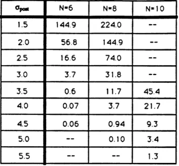
I

Table 2.1: Amplitude of sampling structure for various postfilter standard deviations.

We would like to have the fluctuations of the sampling structure that are produced by the sharpened-Gaussian postfilter in uniform regions to be such that after adaptive demodulation, there are no fluctuations in the noise that is passed in these regions. Sampling structure with an amplitude of between i1 will produce no fluctuations in the adaptation factors in a uniform region when the maximum adaptation factor is 128. This means that the noise will be uniform over that region. Since the postfilter determines the amplitude of the sampling structure, our first step is to fix the standard deviation of the prefilter to some reasonable value (a = 3.0 for N = 6, a = 4.0 for N = 8, o = 5.0 for N = 10), set the standard deviation of the postfilter, and observe the amplitude of the sampling structure in a uniform region of largest magnitude. A unit-step function between 0 and 255 is used for these experiments. The results of this experiment are shown in Table 2.1. For each decimation factor, the amplitude of the sampling structure decreases as the standard deviation of the postfilter increases. For each decimation factor, we should choose the smallest postfilter standard deviation that produces sampling structure with an amplitude of between f1, because a smaller standard deviation will produce a smaller initial overshoot in the highs component, and a smaller overshoot here will allow a faster decay rate when the choice of the standard deviation of the prefilter is made. For decimation factors of N = 6, 8, and 10, we choose a postfilter standard

25 1o N6 N=8 40 NI 1.5 144.9 224.0 --2.0 56.8 144.9 --2.5 16.6 74.0 --3.0 3.7 31.8 --3.5 0.6 11.7 45.4 4.0 0.07 3.7 21.7 4.5 0.06 0.94 9.3 5.0 -- 0.10 3.4 5.5 -- -- 1.3

Overshoot SAplitude 10 10 5 [1 0 2 4 6 8 10

Figure 2.5: Overshoot versus prefilter standard deviation.

deviation of 3.5, 4.5, and 5.5, respectively.

Now that we have selected a postfilter based upon the resulting sampling structure, we need to choose a prefilter, which will be based upon the amount of overshoot and upon the first zero-intercept of the highpass unit-step response. Plotted in Figure 2.5 is the amount of overshoot versus the standard deviation of the prefilter for the postfitlers selected above. Too large an overshoot means that a "halo" of noise will appear several pels away from an edge; however, the smaller the allowed overshoot, the longer will be the extent of the unit-step response. The largest overshoot that produces no noticeable "halo" of noise is approximately 4 to 5. This magnitude of overshoot corresponds to prefiter standard deviations of 4.0, 5.0, and 6.0 for N = 6, 8, and 10, respectively.

For each decimation factor, we have a prefilter and postfilter pair whose unit-step response satisfies the sampling structure and overshoot constraints. Which filter we choose is based upon the spatial/temporal extent of this unit-step response, and we should choose the largest decimation factor whose corresponding unit-step response has an extent of approximately 8 pixels and 8 frames for a 512x512, 60 fps sequence. The location where the step response falls to zero is a measure of the extent of the unit-step response. For N = 6, 8, and 10 and the above corresponding standard deviations, the zero-intercepts are 7, 8, and 12 pels respectively. For a 512x512, 60 fps sequence

26 -ai N 108

/ox

"IT

0-0.4410-aplitude dt U.1 0. ntf -n 1 5 n -25 Prefilter pr = 5.0 -20 Anl i tude B TIC U. 0 0. .1 05 6 -25 -20 -10 0 10 20 i25 i aiH iOulr Postfilter ost = 4.5 -10 0 10 T¥I rmkdrp 20 25

-Figure 2.6: The optimal band-separation Gaussian filter-pair. The standard deviation of the Gaussian prefilter is 5.0, and the standard deviation of the sharpened-Gaussian postfilter is 4.5.

the lowpass component should be calculated by using a Gaussian prefitler of standard deviation 5.0, a sharpened Gaussian postfilter of standard deviation 4.5, and a decimation factor of 8. This filter and its unit-step response are shown in Figure 2.6. Figure 2.7 shows the original CMAN and GIRL pictures, and Figure 2.8 shows two 2-D highpass and two decimated 2-D lowpass images produced by this filter-pair.

Because of the long length of this filter pair, its use in the temporal direction is im-practical. The shortest filter pair that produces the desirable decay rate is the averaging prefilter and the linear postfilter. This filter pair produces a unit-step response that has linear decay and a zero-intercept at 8 pels. The decay rate corresponding to the Gaussian filter pair is faster than that corresponding to the linear filter pair.; however, the length

27 - I --- ... ·- ·- --.I... .··--bz= I.... ... _ ns .PPC-.. . . _ .. ... ... T... ... ... I...I ... ... ns .-. . - --'cCctjSeSL/

vti9ee'S"

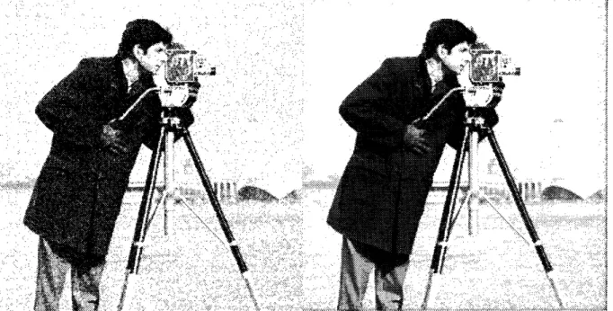
Figure 2.7: The original CMAN and GIRL pictures.

of the linear postfilter is much shorter and can be implemented in a cascade structure to reduce the required number of frame stores. Figure 2.9 shows the 2-D lowpass and highpass frequency components produced by this filter pair.

2.2

Calculating the Adaptation Factors

Now that we have settled upon a filter pair to perform the band separation, let us take a closer look at how the adaptive modulation is performed. Since one adaptation factor (or modulation index) is calculated for every 3-D block of image data, the sequence

ps[ml, M2, m3] can be considered as a type of subsampled, or decimated, sequence of the

input highs, ih[nl, n₂, n3]. The subsampled data can be written as,

ps[ml, m2, m3] = S[ih[nl, n2, n3]]. (2.4)

The subsampled indices, mi = f[], denote the integer part of the fraction. The operator S calculates a single sample for an NlxN2xN3 block of data in the horizontal, vertical,

...

Figure 2.8: The highpass response of CMAN and GIRL using the final Gaussian filter-pair. The decimated lowpass images are also shown. The highpass components have an offset of 128.

:~::X::a:I:::I:i:a:::::::::::::::::::: : = = ================================= ": ;$:::7i:;_{... ... .. ... .. ... ... . ... .. .. .. .. ."* " ~ ' * *...... .. ...} i~~~~Il~~~~~ii .~~~~~~... ... . :.::if: "~ ... F '"'".'"', ... ~..~...~.~~~~i~ i.`.::..:,:~~..~ ".,.~ ~~ : ...

Figure 2.9: The highpass and decimated lowpass components of CMAN using an

aver-aging prefilter and a linear postfilter. Notice the aliasing. The highpass component has

an offset of 128. ·BBbi:ii _d ::u I::: · ·: iX :::: :: i8r :·: :: .>si:5 ~ Is : M; } sa.:.s Y , :,Sr: "::::,: :s u::,:: ,,:::':::: :.:. .. .::::: ;s w.. r... >.Y,

and temporal directions, respectively, and may include prefiltering prior to subsampling. The sequence, p,[ml, m2, 3] is interpolated by N1, N2, and N3 to form the sequence

p[nl, n2, n3], and the adaptation factors are calculated as

m[ni, n2, n31 = f(p[nl, n2, n3]) (2.5)

for some function f. The sequence of adaptation factors m[ni, n2, n3s] is multiplied with

ih[nl, n2, n3] to form y[nl,n2, n3]. This new sequence is expanded and then clipped to

±:ihmax if the signal exceeds this range, where ihmax is the absolute maximum value that i[nl, n2, n3] is assumed to attain. For image data with a dynamic range from 0 to

255, the largest absolute value that the highpass component can attain is 255, although values over 128 for normal images are rare. The maximum value, ihmax, is chosen so as not to have significant distortion due to clipping but yet to have a sufficient blank area signal-to-noise ratio (SNR). Normally the maximum value is set to 128. Clipping y[nl , 2n31 will produce distortion in the demodulated output, [nl, n, n3], which will show up as a softening or blurring of the picture.

Now, let us introduce a set of adaptation factors for which the sequence y[nl, n2, n3] is

clipped only when ih[nl, n2, n3] > ihmax, and the adaptation factors are the largest they can be given this condition. This distinction is important because the clipping arises only from our choice of ihmax and not from subsampling or interpolation. This set of adaptation factors is

mmax for hmax >mmax

mo[ni, n2, n3] = lih[lnnajll > (2.6)

-hlin - otherwise,

where the subscript, o, indicates the "ideal" adaptation factors and mmax is the largest value we will let the adaptation factors attain. Multiplying the input data, ih[nl, n2, n3], with m[nl,n2,n3] would use the channel most efficiently; however, the amount of side information would be as much as that required to send the input data itself. This is why we need to subsample the input data and interpolate it in calculating the adaptation factors. An example of an adaptive modulation algorithm is that proposed by Schreiber and Buckley [SB811. The subsampling operation they use is

for [nl, n2, n3s] which are elements of an NxN2xN3block. The subsampled data, p,[ml, m2, m3],

are linearly interpolated with the sample located in the center of the block, and the adap-tation factors are calculated according to

Mmax for K >M

m[ni, n2, n3] =

f

L[-K ,,2,]I otherwise,

where K is set to a value that causes negligible distortion in the worst case. This value is set to 60.

Because of subsampling and interpolation, the sequence of adaptation factors, m[ni, n2, n3],

differs from the ideal adaptation factors, mo[nl, n2, n3]. In some instances, m[ni, n2, n3]

will be greater than mo[n1, n2, n3] and in others, less than m[nl, n2, n3]. In those cases

where m[ni,n2, n3] > mo[n, n2,n 3] (i.e., where I p[nl,n2,n3]

1<1

ab-solute value of the product of m[nj, n2, n3] and ih[nl, n2, n3] will be greater than ihmax,

and distortion will occur in the demodulated output due to the subsampling and inter-polation operations. Having m[nj, n2, ns] > m[nl, n2, n3] is not entirely undesirable; in

fact, it should be weighed against the increase in noise-reducing capability that having a larger m[n1, n2,ns] over the ideal case will produce. Having m[n,, n2, n3] > mo[n, n2, n3]

for certain picture elements will tend to raise the value of adaptation factors of neighbor-ing picture elements without distortneighbor-ing those picture elements. For example, in regions near an edge, some picture elements will have adaptation factors larger, and some smaller, than the ideal adaptation factors due to the interpolation . By allowing more distortion of the picture elements with larger adaptation factors, the noise-reducing capabilities of picture elements with smaller adaptation factors near edges is increased without distort-ing those picture elements. If the distortion is not noticeable, then we have increased the overall noise-reducing capability without visibly degrading the demodulated output image, [nl, n2,n3]. Little work has been done in finding this threshold of tolerable

dis-tortion or in using different types of subsampling operations or interpolation methods. Before we investigate the subsampling (decimation) and interpolation processes, it is instructive to look at the signal as it evolves through the adaptive modulation pro-cess for the adaptive modulation algorithm used by Schreiber and Buckley. Figure 2.10 shows various signals of the adaptive modulation process for line 51 of CMAN. The band

Anplitude H ighpss Conponent 100 -100 40 30 20 10 160 170 180 190 200 Apl itude Adaptation Factors 160 170 180 190 200 Apl itude

Nosy Adaptiveity Modulated Hi

0 0 160 170 ighs 180 190 200 Amplitude .^^ Interpolate SubsampLes

(a)

daptivey odulated Highs

(C)

.. .... ..

(e)

Figure 2.10: Evolution of signals in the adaptive modulation process.

33 LAI -20O (b) Pal num*%ar C 10

tKP

I.WI

(f)

t"c

...-.... ...-... ...-...-...I...

) ... A--'

M ,

-....

...

...

...

...

ATV

I 'iV ,

separation is performed with the filter pair from the previous section, where the low-pass signal is decimated by 8 in both the vertical and horizontal directions. No filtering is performed in the temporal direction. Schreiber and Buckley subsample the highpass component, ihnl, n2, n3] (Figure 2.10(a)), by finding the maximum of the absolute values

in a 4x4 spatial block of the highpass signal and interpolate using a bilinear filter to

pro-duce p[ni, n2,n 3] (Figure 2.10(b)). The adaptation factors, m[nl, n2, n3], are calculated

according to eqn. 2.8 with K = 128 and are shown in Figure 2.10(c). Here, we have allowed the maximum adaptation factor to be 128. Multiplying the highpass component,

ih[nl, n2, n3], with the adaptation factors, m[nl, n2, n3], produces the adaptively

modu-lated signal, y[nl, n2, n3], as shown in Figure 2.10(d). If the noise in the channel has a 20dB CNR, then the signal in Figure 2.10(e) results. The adaptively demodulated sig-nal, h[ni, n2, n3], is shown in Figure 2.10(f). The entire highpass component of CMAN,

its adaptation factors, and the adaptively modulated highpass component are shown in Figure 2.11, and the demodulated pictures which result when no adaptive modulation is used and when adaptive modulation is used over a 20dB CNR channel are shown in Figure 2.12.

How does adaptive modulation change the characteristics of the highpass signal? Three characteristics of interest are the histograms, the power spectra, and the energies of the signals. The histogram of the highs component is shown in Figure 2.13(a). As one would expect, most picture elements have very small values. Adaptive modulation, in its ideal form, should raise the value of each pel, except 0, to imax = 128 but is limited by the value of the maximum adaptation factor, which we have set to 128. Figure 2.13(b) shows the histogram of the adaptively modulated highs. Figure 2.14 shows the power spectra of the highs component and of the adaptively modulated highs component. The standard deviation of the highpass component is 43.2, and the standard deviation of the adaptively modulated highpass component is 69.2. For comparison, the standard devi-ation of the original, fullband CMAN is 68.6. Although adaptive moduldevi-ation increases the energy of the highpass component, it does not change the peak power of the signal.

During all of our experiments on adaptive modulation, we set the length of any one side of the 3-D block to be one half the decimation factor used when decomposing the

A

Figure 2.11: Highpass component, adaptation factors, and adaptively modulated high-pass component of CMAN. An offset of 128 has been added to the highhigh-pass component

and to the adaptively modulated highpass component. The adaptation factors have been scaled by 4.

Figure 2.12: Demodulated signals when no adaptive modulation is used and when

adap-tive modulation is used when transmitting over a 20dB CNR channel.

·.· · __ :.i. :i:i '21 qi 2.::?!i .:: I:S -.. .,-.2

Nurber of Pets -nn ,UUU 2000 1000 0 -128 -100 -50 0 50 10 (a) A. i At o ₁₀₁₂₈1 '-... urmber of Pets --AA. 3UUU 2000 1000 0 -128 -100 -50 0 50 (b) Ainl itde 100 j128

Figure 2.13: Histograms of the highpass (a) and adaptively modulated highpass (b) components of CMAN.

Magnitude edB)

-64 -50 -25 0 25

Figure 2.14: The horizontal frequency axis of the power adaptively modulated highpass components of CMAN.

Highs

[ti/I4 rad/sec)

SO 6-

spectra of the highpass and

37

I

I....

----_i

- i

I

__

!---

input signal into lowpass and highpass components. For a 512x512, 60 fps sequence the decimation factor is 8 in each dimension; therefore, our block size will be 4x4x4. The rate of decay of the interpolated subsamples, p[nl, n2, n3], determines the block size.

When the peak value of the highpass component within a block occurs in the middle of the block, then, depending upon what interpolation method is used, the effect of the peak upon the rate of decay of the interpolated subsamples can extend up to twice the length of the block along each dimension. Since we would like the rate of decay of the interpolated subsamples to coincide with the effects of masking, we choose the length of each side of the block to be one half the decimation factor used during band separation. In addition, we use the function described in eqn. 2.8 with K = ihmax = 128 to calculate the adaptation factors.

2.3

Origins of Distortion

Before we embark on the discussion of our experiments on subsampling, interpola-tion, and distorinterpola-tion, let us explore the origins of distortion. The transmitter must clip the adaptively modulated signal prior to transmission in order to conform to the peak trans-mission power constraint for broadcasting television signals; therefore, distortion occurs when the adaptively modulated highpass component, y[nl, n2, n3], is above imax, which happens either when the highpass signal, ih[nl, n, na], is above ihmax or when the adap-3

tation factors, m[ni, n2, n3], are larger than the ideal adaptation factors, m[n, n2, n3].

This latter condition occurs when the absolute value of the interpolated subsamples,

I p[nl, n, n3] I, are smaller than the corresponding absolute value of the highpass

sam-ples, I ih[nl, n2, n3] . Without loss of generality, let us consider only positive values and

suppose p[nl, n, 3] < ih[nl, n, n3] and

p[nll,n2, n3] = ih[nl,n n2, n3]- Aih[nl, n2, 73] (2.9)

for some ni, n2, and n3, and where Aih[nl, n2, n3] > 0. Under these conditions, distortion occurs. The adaptation factor is

128

mn,n 2, n3] = 128

i[nl, n3]- i[nl, n2, n3] (2.10)

where we assume that 1 < p[nl, , n] n3 < 128. The adaptively modulated sample is

y[nl, n2, n3] = ih[nl, n2,n3]m[n, n2, n3]

128 128 Aih[nl, n2, n3]

h[n1n2,n3](ih[n, n, n3] ih [ni, n2, n3](ih[nl, n2, n3] - ih[nl, n2, n3]))

=

128 + 128 Aih[nl, n2, n3] (2.11)

ih[n, n2, n3] - Aih[nl,n2, n' 3]

which is > 128. The second term is the amount of the signal which gets "clipped off." The received sample is

[nl, n, n3] = 128 + v[nl, n2, n3] (2.12)

where v[nl, n2, n3] is additive noise. The demodulated sample is

ih[nn, n , 3] 2

m[nl,n2, n3]

128 + v[nl, n2, n3 , ], , )

(ihl, 2,n] - ih[,2,3])

(ih[nl, n2, n3]-Aih[nl, n2, n3])

v[ni, n2, n3](ih[nl, n2, n3] - Aih[nl, n2, n3]) (2.13)

128

The first term is the distorted highpass signal and the second term is the reduced noise. The distortion is ih[nl, n2, n3], which is just the difference between the highpass

sam-ple, ih[ni, n2, n3], and the interpolated subsample, p[nl,n2, n3], when I p[nl, n2, n3] <

I ih[nl,n2,n3] [. When [ p[nl,n2,n3] I > ih[nl,n2,n3l] , no distortion occurs. This is

shown pictorially in Figure 2.15. To increase noise reduction, we want Aih[nl, n2, n3] to

be as large as possible; however, to reduce distortion, we want Aih[nl, n2, n3] to be as

small as possible.

2.4

Decimation and Interpolation of the Highpass

Component

The existing adaptive modulation algorithm, which was put forth by Schreiber and Buckley, allows negligible distortion due to clipping to occur. Under bad (< 25dB CNR)

distortion occurs

Number

Figure 2.15: Distortion occurs when the absolute value of the interpolated subsamples is less than the absolute value of the highpass samples.

noise conditions, this algorithm does not sufficiently suppress the noise around edges (see Figure 2.12.) Two ways to improve the performance of adaptive modulation is to increase the rate of decay of the interpolated subsamples by using a sharpened interpolating filter and to allow more distortion to occur.

In our first set of experiments, we subsampled by finding the maximum of the absolute values of the highpass component in a block (Schreiber and Buckley's method) and interpolated with a sharpened-Gaussian filter. Sharpened-Gaussian filters with standard deviations from 1.5 to 2.5 were tried (see [Rat80] for formula of a sharpened-Gaussian filter). No improvement over using a bilinear interpolating filter was found. In fact, the pictures looked worse because using sharpened Gaussian filters resulted in large overshoots and sampling structure, which manifested themselves as significant distortion in the demodulated output. Using the nonlinear mechanism of finding the maximum absolute value in a block as the subsampling operation does not sufficiently bandlimit the signal, so that significant aliasing occurs when interpolating with a sharpened filter. The aliasing shows up as strong ringing. One way to circumvent this problem is to

use a subsampling operation that better bandlimits the signal. Buckley also performed experiments where he varied the interpolating filter; however, none of his filters were sharpening filters. He similarly found that when using the maximum absolute value in a block as the subsampling operation, a linear interpolating filter gives the best looking pictures.

Prefiltering prior to using the conventional subsampling operation,

p[m, m2, m 3 = S(ih[nl, n2, n3]) = ih[mlN, m2N, m3N3] (2.14)

where NlxN2xN3 is the block size, should allow the use of sharpened-Gaussian filters

to increase the decay rates of the interpolated subsamples without the large ringing and overshoots. We limit ourselves to Gaussian prefilters and decimate and interpolate only the absolute value of the highpass component to find p[nl, n2, n3]. Using the

max-imum absolute value in a block and linear interpolating produces negligible distortion; whereas, using conventional decimation and interpolation operations can produce signif-icant amounts of distortion. This in itself is not bad. To reduce the distortion one only needs to scale p[nl, n, n3s] by some factor to produce any desired level of distortion. This

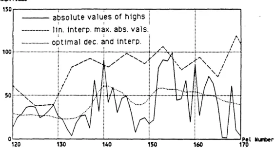
is done in latter experiments. What is important is that the p[n, n2, n3] that results

when using Gaussian prefilters and sharpened-Gaussian postfilters somehow better

fol-low the fluctuations of ih[nl, n2, n3a compared to the p[nl, n2, n3] that result when using

linear interpolation of the maximum absolute values. This statement is hard to quantify, and a good filter-pair can only be found by subjective judgment.

The prefilter controls the amount of high-frequency information that gets passed. Too small a standard deviation of the Gaussian prefilter will allow too much aliasing and too much overshoot after interpolation. Too large a standard deviation of the prefilter will excessively blur the edges and will decrease the rate of decay of the impulse response of the interpolated subsamples. The postfilter controls the band separation properties, visibility of sampling structure, and the sharpness of edges. A large standard deviation of the postfilter will produce fast transitions and large overshoots, which are undesirable because they produce a "halo" of noise around sharp edges. Small standard deviations of the postfilter have poor band-separation properties, and sampling structure becomes