Differentiable Physics and Stable Modes
for Tool-Use and Manipulation Planning
The MIT Faculty has made this article openly available.
Please share
how this access benefits you. Your story matters.
Citation
Toussaint, Marc et al. “Differentiable Physics and Stable Modes for
Tool-Use and Manipulation Planning.” Proceedings of the Robotics:
Science and Systems, RSS 2018, Pittsburgh, Pennsylvania, June
26-30, 2018 © 2018 The Author(s)
As Published
10.15607/RSS.2018.XIV.044
Publisher
Robotics: Science and Systems Foundation
Version
Author's final manuscript
Citable link
https://hdl.handle.net/1721.1/126626
Terms of Use
Creative Commons Attribution-Noncommercial-Share Alike
Differentiable Physics and Stable Modes for
Tool-Use and Manipulation Planning
Marc Toussaint
†∗Kelsey R. Allen
∗Kevin A. Smith
∗Joshua B. Tenenbaum
∗∗Massachusetts Institute of Technology, Cambridge, MA 02139
{mtoussai,krallen,k2smith,jbt}@mit.edu
†Machine Learning & Robotics Lab, University of Stuttgart, Germany
Abstract—We consider the problem of sequential manipulation and tool-use planning in domains that include physical interac-tions such as hitting and throwing. The approach integrates a Task And Motion Planning formulation with primitives that ei-ther impose stable kinematic constraints or differentiable dynam-ical and impulse exchange constraints at the path optimization level. We demonstrate our approach on a variety of physical puzzles that involve tool use and dynamic interactions. We then compare manipulation sequences generated by our approach to human actions on analogous tasks, suggesting future directions and illuminating current limitations.
I. INTRODUCTION
In this paper we address manipulation planning problems that involve sequencing constrained interactions such as stable pushes with a tool or sliding an object along a wall, as well as dynamic interactions such as hitting a ball in the air. These creative manipulation capabilities are a hallmark of intelligence. Betty the Crow (see Fig. 1 top-left) demonstrated the ability to use a sequence of hooks to retrieve a piece of food [33], and Koehler’s apes stacked crates to reach a hanging bunch of bananas (bottom-left) [12]. Humans easily perform such sequential manipulation planning tasks naturally and flexibly (bottom-right).
Evidence from cognitive science suggests that people have an “intuitive physics engine” [2] which can be used to simulate the outcome of an action or tool manipulation [22], and have dedicated neural architectures near the motor cortex for implementing this capability [8]. But a typical physics engine only predicts outcomes for an action, not how to choose those actions.
Consider if we had a precise and efficiently invertible physical simulator available. Candidates for this were proposed in terms of fully (auto-) differentiable physical simulations [29, 7], which have the potential to embed control synthesis and planning within end-to-end trainable systems [28]. Invert-ing a simulation means that we can in principle formulate any objectives or constraints on the end result or trajectory of the simulation and solve for the inputs (control signals of an embedded robot, or parameters of the scene or kinematics) that render the desired constraints true. For instance, if we could efficiently invert a correct physical simulation, we could constrain the end result to be a cleaned-up kitchen and solve for the motor inputs that make a PR2 reach this state starting from a messy kitchen.
Fig. 1. From left to right: A crow solving a sequential hook problem [33], classical intelligence test with apes [12], our solver using a stick to hit a flying blue ball to get it into the green area, using a hook to get a second hook to reach for the red ball, a human subject on the same task.
Unfortunately, efficient general inversion of a physical sim-ulator is implausible as it defies what we know about the fundamental complexities of task and path level planning [15], as well as control synthesis. The complexity of inverting a physical simulator is implicit in the non-unimodality of the resulting optimization problem. In sequential manipulation, the underlying structure is determined by contacts or—on a higher level—by decisions on which object is manipulated and how. Both imply discontinuities in the physical effects and local optima w.r.t. the global inverse problem. Our approach is to explicitly model such structure:
Approach 1: Use logic to express the combinatorics of possible physical interactions and respective local optima. This follows the paradigm of Mixed-Integer Program (MIP) formulations in hybrid control synthesis [5]. However, it ex-tends this to 1st-order logic, leveraging the strong generaliza-tion over objects of classical AI formulageneraliza-tions. It also follows the standard task and motion planning (TAMP) approach of using logic to describe the task level, but now describes the combinatorics of possible physical interactions.
In addition, a precise physical simulation is very powerful as it can predict many kinds of interactions, including high frequencies of contact switches. Eventually, we are not in-terested in modeling anything possible, but rather in modeling interactions that are useful for goal-directed manipulation. The classical manipulation literature emphasizes the importance of stable interaction modes and funnels [19, 17, 3]. A mode can mean that contact activities are phase-wise constant [21], but also that the relative transformation between objects is held constant, allowing for a kinematic abstraction of the interaction. We adopt this view in our approach:
Approach 2: Restrict the solutions to a sequence of modes; consider these as action primitives and explicitly describe the kinematic and dynamic constraints of such modes.This dras-tically reduces the frequency of contact switches or kinematic switches to search over, and thereby the depth of the logic search problem. It also introduces a symbolic action level following the standard TAMP approach, but grounds these actions to be modes w.r.t. the fundamental underlying hybrid dynamics of contacts.
Combining the two approaches, the core of our method is to introduce explicit predicates and logical rules that flexibly de-scribe possible sequences of modes, mixing modes that relate to physical dynamics for some objects and stable kinematic relations for others. All predicates are grounded as smooth and differentiable constraints on the system dynamics. Leveraging an optimization-based TAMP method, this enables efficient reasoning across a spectrum of manipulation problems. We demonstrate our approach on physical puzzles that involve tool use and dynamic interactions such as inertial throwing or hitting. We also collected data of humans solving analogous trials, helping us to discuss prospects and limitations of the proposed approach.
II. RELATEDWORK
Differentiable Physics & Contact-Invariant Optimization: [7] have recently observed that a standard physical simula-tion, which iterates solving the linear complementary problem (LCP), is differentiable and can be embedded in PyTorch. On toy problems it was shown that, using gradient-based optimiza-tion, one can infer controls or scene parameters conditional to observations or desired effects. Earlier, Todorov introduced a novel invertible contact model [29] that laid the foundation for MoJuCo [30], a differentiable physics engine that allows for inverse physical dynamics. Closely related, contact-invariant optimization (CIO) [21] proposes a simplified differentiable contact model that relaxes the discrete contact structure to
allow for smooth optimization, but still implies a combina-torics of local optima of the general inverse problem. CIO gave impressive demonstrations of complex human motions, including typical locomotion optimization and manipulation tasks. CIO also followed the approach of phase-wise contact invariance, where the (continuous-valued) activity of a contact interaction is constrained to be constant during a phase.
These methods have not yet been demonstrated to bridge to higher-level tool-use or task planning, and have not been integrated in AI planning or TAMP approaches. They reduce the overall problem to a single (differentiable) non-linear program, which seems promising only when the underlying problem does not generate a combinatorics of local optima.
Mixed-Integer Programming in Hybrid Control: In control synthesis the structure of hybrid contact processes is typically described explicitly [5] (see also [23] for a critical discussion). The resulting problems are MIP that can be addressed with standard optimizers that typically involve branch-and-bound. Our approach is similar, except that we use logic rules to describe the discrete structure of the problem, leading to a non-linear program with discrete 1st order decision variables (in a sense a “Mixed-Logic Program”). The solver we use [32] is very similar to branch-and-bound MIP solvers, but leverages several bounds approximations for computational efficiency.
Posa et al. [23] criticize explicitly introducing discrete decision variables and instead propose non-linear programs without discrete variables for the overall path optimization problem (using LCP-type terms). This follows CIO in avoiding discrete structure, but also raises the question of local optima in task-level domains.
None of the above control approaches have yet been demon-strated to bridge to higher-level task-planning and tool-use.
Task and Motion Planning:Typical TAMP approaches rely on a discretization of the configuration space or action/skeleton parameter spaces to leverage constraint satisfaction methods [16, 13, 14], and/or combine a standard sample-based path planner with a task planner [27, 4, 1]. To our knowledge, no prior work exists that aims to integrate dynamic physical interaction or sequential tool use in TAMP methods. Comput-ing physical paths in a high-dimensional configuration space (our robot will be 14D) is hard to address using sample-based planners. Toussaint and Lopes [31, 32] proposed an optimization-based TAMP approach that combines a logic task-level description with a non-linear programming formu-lation of the resulting path optimization problem. We extend this framework to include physical primitives.
Exploitation of Contacts in Manipulation:Exploiting rather than avoiding contacts is a core concept for dexterous robot manipulation [19]. Stable pushes [17] and sequences of stable grasps [3] have been shown to enable robust manipulation strategies. Eppner et al. [6] studied in detail how humans exploit contacts in manipulation. The idea that exploitation-of-contact-modes should be part of a manipulation planner underlies previous work on sequential manipulation planning [26, 10]. Sieverling et al. [25] further developed the idea towards sequencing modes to reduce uncertainty via funneling.
Our approach draws great inspiration from these works, aiming to incorporate such ideas in an AI- and optimization-based planning approach.
III. PROBLEMFORMULATION ANDLGP FORM
Consider the configuration space X = Rn × SE(3)m of
an n-dimensional robot and m rigid objects, in an initial configuration x0∈X. We aim to find a path x : [0, T ] → X
min x Z T 0 fpath(¯x(t)) dt + fgoal(x(T )) s.t. x(0) = x0, hgoal(x(T )) = 0, ggoal(x(T )) ≤ 0 , ∀t ∈ [0, T ] : hpath(¯x(t)) = 0, gpath(¯x(t)) ≤ 0 . (1)
Here, (h, g)path define path constraints which depend on
¯
x(t) = (x(t), ˙x(t), ¨x(t)) and describe what is physically and kinematically feasible. The function fpathdefines control costs,
which in our experiments we choose as sum-of-squares of joint accelerations. And (f, h, g)goal specify arbitrary objectives or
constraints on the final configuration. In our experiments this will be a single equality constraint expressing contact between an object and a target.
Following our approach, we now introduce more structure to the problem. We assume that 1) feasible mode transitions are described by first order logic action operators, 2) in a given mode the path constraints (h, g)path are smooth, and 3) at a
mode transition the path constraints are smooth functions of ˆ
x = (x, ˙x, ˙x0), where ˙x is the velocity before, and ˙x0 is the velocity after an (optional) instantaneous impulse exchange. Under these assumptions, the problem takes the form of a Logic-Geometric Program (LGP) [31, 32], min x,a1:K,s1:K Z T 0 fpath(¯x(t)) dt + fgoal(x(T )) s.t. x(0) = x0, hgoal(x(T )) = 0, ggoal(x(T )) ≤ 0, ∀t ∈ [0, T ] : hpath(¯x(t), sk(t)) = 0, gpath(¯x(t), sk(t)) ≤ 0 ∀k ∈ {1, .., K} : hswitch(ˆx(tk), ak) = 0, gswitch(ˆx(tk), ak) ≤ 0, sk∈ succ(sk-1, ak) . (2)
The key difference to the unstructured problem (1) is that the path and switch constraints (h, g)path and (h, g)switch are
smooth and differentiable functions for a fixed mode sk or
switch ak. We assume that the logic level involves only
discrete variables (in contrast to recent TAMP approaches that introduce continuous logic variables to represent belief or geometry dependent preconditions [16]). All ak and sk
are therefore discrete. We call the sequence a1:K a skeleton,
which in the TAMP context refers to the sequence of dis-crete decisions excluding all continuous action parameters. In TAMP, given a skeleton, one needs to find action parameters (e.g. grasp poses) that render the skeleton feasible. In our formulation, we use the notation P(a1:K) to denote the path
optimization problem (2) for a given skeleton. As (h, g)path
and (h, g)switch are smooth, all objectives and constraints in
P(a1:K) are smooth and our implementations are differentiable
to provide constraint Jacobians and pseudo-Hessians when the costs fpath,goalare sum-of-squares terms. Solving P(a1:K)
im-plicitly solves for all action parameters jointly and optimally: E.g. when the sequence involves a grasp first, a hit second, and a placement third, then all parameters of these actions (grasp pose, hitting angle, placement pose) are jointly optimized to yield the overall optimal manipulation path.
The LGP formulation can be viewed as an instance of MIP, as it is classically used to formulate control problems in hybrid systems [5]. It replaces integers by a first order logic state sk
which indicates the mode, and thereby allows us to tie the notion of high-level actions of a classical TAMP formulation to modes in the path optimization problem. In contrast to CIO it explicitly introduces a logic process description of mode transitions that bears a discrete search problem. It thereby explicates the structure of local optima that is otherwise implicit in the relaxation.
Comparing 2 to the previous formulation [32], the path constraints within a mode are now functions of ¯x, rather than only (x, ˙x), as they need to describe inertial motion, and the switch constraints are functions of ˆx to account for impulse exchanges. We also explicitly refer to the action decision ak
rather than only pairs of consecutive modes (sk-1, sk) to define
switch constraints. To motivate these additions, consider a flying ball which is hit with a tool in the air. The modes before and after the hit are identical; there were no kinematic switches or stable contacts created. However, the interaction calls for an equality constraint on the path that models contact and impulse exchange.
In practice, to ensure applicability of the solver, we assume that each object has a sphere-swept convex geometry (which makes distance computation convex, and ensures distance normals to be differentiable).
A. The Notion of Modes
The previous section defined a specific notion of mode in terms of properties of the path constraints. To better relate to previous work we briefly discuss highly related notions.
A contact mode is a phase of the path where contact activations are constant (cf. CIO [21]). In classical con-strained optimization and LCP formulations, contact activation is boolean and indicates a non-zero Lagrange parameter or non-zero interaction force; in CIO contact activity is relaxed to a continuous number, which is kept constant within a contact mode.
A kinematic mode is a phase of the path during which path feasibility (including physical correctness) is defined by smooth constraint functions hpath, gpath. To relate to [26,
10, 32], the path constraints define the piece-wise smooth manifolds of feasible paths with local tangent spaces TzX =
{ ˙x(t) | x(t) = z, x feasible} at configuration z ∈ X; a kinematic mode is a phase during which the path stays within a smooth manifold. Transitioning to another mode implies a non-smooth change of tangent space.
A stable mode is a phase of a feasible path in which the relative transformation between two objects is constant. This
refers to resting objects, but also to stable pushes [17, 3] and grasps.
In the case of a physical domain, feasible paths are smooth exactly when contact activity does not alter, and therefore the two notions of contact mode and kinematic mode coincide. A stable mode is a special case of a kinematic mode, which excludes sliding, relative rotation, and impulse exchange. However, the manipulation literature suggests that many ma-nipulation strategies are composed of stable modes, which mo-tivates us to explicitly account for stable modes. Stable modes offer transitions between kinematic and dynamic descriptions of the path constraints by, for example, introducing a joint between two objects that is constrained to zero velocity. Note that in CIO [21], all contacts were in fact assumed to be stable modes.
The core of our approach is to introduce predicates and logical rules that flexibly describe possible sequences of modes, mixing modes that relate to physical dynamics for some objects and stable kinematic relations for others.
IV. INCORPORATINGPHYSICS INLGP
Table I lists the predicates we use to impose constraints on the path optimization. These relate the logic level to the path optimization level, and appear only in the effects of action operators. We will first describe these predicates, and then the action operators that control them.
A. Resting and Stable Relations
In typical scenes, most objects are resting in a stable position or in a grasp. Including their degrees of freedom in the optimization and solving for the contact interactions in each time step—only to describe zero motion—is inefficient. Typical game engines therefore treat resting objects differently from dynamic objects.
We follow this intuition and exclude objects resting on another object or in a grasp from physical dynamics. These objects are treated kinematically, as in previous work. Namely, operator effects create a static joint between the object and its parent. For our experiments, it was sufficient to consider only two types of static joints: static free (represented as 7D translation-quaternion joints) for grasping, (staFree X Y), and static “on” (represented as 3D xyφ-translation-orientation joints) for an object resting on another, (staOn X Y).
As in typical path optimization methods we use a (gener-alized) coordinate vector q(t) ∈ Rd(t) to represent the world
configuration x(t) ∈ Rn× SE(3)m. While x(t) is of constant
dimensionality, q(t) changes dimensionality with t. When all objects are initially at rest, q(0) has the dimensionality of the articulated robot. When action operators create stable or dynamic joints their degrees-of-freedom (DOFs) are added to the configuration vector. The static joints are introduced as DOFs, but are constrained to have zero velocity. Thereby they represent action parameters (e.g. grasp poses) that are fully embedded as decision variables in the joint path optimization.
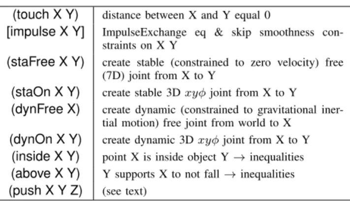
TABLE I
PREDICATES TO IMPOSE CONSTRAINTS ON THE PATH OPTIMIZATION.
(touch X Y) distance between X and Y equal 0
[impulse X Y] ImpulseExchange eq & skip smoothness con-straints on X Y
(staFree X Y) create stable (constrained to zero velocity) free (7D) joint from X to Y
(staOn X Y) create stable 3D xyφ joint from X to Y
(dynFree X) create dynamic (constrained to gravitational iner-tial motion) free joint from world to X
(dynOn X Y) create dynamic 3D xyφ joint from X to Y
(inside X Y) point X is inside object Y → inequalities
(above X Y) Y supports X to not fall → inequalities
(push X Y Z) (see text)
B. Inertial Motion
To describe objects following inertial motion, operator ef-fects create a dynamic joint between the object and world (for unconstrained flight) or supporting objects (e.g., for inertial sliding on a table). In our experiments we consider two types of dynamic joints: 7D free for free flight, (dynFree X), and xyφ for one object sliding on another, (dynOn X Y). For the set qdof dynamic joints we have the Euler-Lagrange equations
M (q)¨qd+ F (q, ˙q) = 0 (assuming kinematically articulated
and stable joints to be rigid), which are imposed as equality constraints on the path. In the time discretized path optimiza-tion, care must be taken in deciding when to start and stop imposing these constraints when dynamic joints are created or destroyed. In the time slice when a joint switches, we generally impose zero acceleration constraints directly on the switching object (except on impulse exchange); the dynamics constraints start a time step later and end one time step earlier. The acceleration ¨qdis defined by finite differences from three
consecutive configurations. The dynamics constraint is trivially differentiable w.r.t. these configurations, assuming M and F are approximately constant.
C. Impulse Exchange
To model impulse exchange we introduce an[impulse X Y]
predicate, where the bracket notation indicates that it is non-persistent. Unlike in the standard frame assumption, this literal is automatically deleted after one time step. It thereby adds constraints to the path optimization only at a single time slice (but is a function of 3 consecutive configurations). We adopt the classical impulse exchange model of Moore and Wilhelms [20]. Let v1 and v2be the change in velocities of object 1 and
2 across one time slice, and ω1 and ω2 the angular velocity
changes. We define the exchanged impulse as R = m2v2.
(If (3) holds, we could equivalently define R = −m1v1.)
Further let c be the shortest distance or penetration unit normal vector between the two convex objects, and p1 and p2 the
unconstrained case we impose
m1v1+ m2v2= 0 (3)
I1ω1− p1× R = 0 (4)
I2ω2+ p2× R = 0 (5)
(I − cc>)R = 0 (6) where the last line constrains the exchanged impulse to align with the contact normal. In an inelastic collision we additionally impose zero relative velocity along the contact normal, which we drop to allow for elastic collisions. When the dynamics of one object is constrained to an xyφ slide after the impulse exchange, we project the first equation using the projection matrix P = I − zz>where z is the plane normal. This means that the impulse is not propagated through the joint to the supporting object (typically table).
To ensure differentiability of this constraint we extend implementations of Gilbert-Johnson-Keerthif and Minkowski Portal Refinement to return simplex information from which the correct Jacobian for the distance or penetration normal vector is computed. As our objects are modeled as sphere-swept convex shapes, these Jacobians are stable and smooth at distance 0. Therefore the full impulse exchange constraint is smoothly differentiable.
D. Geometric Predicates
We additionally introduce three geometric predicates(touch X Y), (inside X Y), and (above X Y) to model constraints of transitioning into a mode. Atouchis modeled by constraining the differentiable distance or penetration function to zero. The
inside constraint means that a grasp center X is constrained to be inside the object Y (by a fixed margin of 2cm). When Y is a box, these are six inequality constraints, one for each face of the box. The above constraint requires the center of mass of X to be horizontally inside the convex support the object Y (by a fixed margin of 2cm). When the supporting object is a table, these are four inequality constraints, one for each edge of the table. Finally, the (push X Y Z) predicate is designed specifically to impose geometric constraints for a straight-linepush. It is modeled kinematically by introducing a static xyφ-joint and an actuated translational x-joint created between table Z and object Y, which allows the object to move along a straight line. Further, the pushing object X and Y touch and the touch normal is aligned with the straight line.
In summary, the predicates we introduced allow us to distinguish and switch between dynamic and kinematic han-dling of objects. Modeling stable relations explicitly allows us to include abstractions such as stable grasping or stable resting. The geometric predicates allow us to define necessary geometric constraints to transition between modes.
E. Action Operators
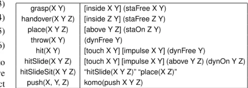
Table II lists all action operators and those effect predicates that translate to path constraints. We briefly discuss each action:
A grasp creates a 7D static gripper-object joint and imposes the grasp center to be inside the object. The inside constraint
TABLE II
ACTION OPERATORS AND THE PATH CONSTRAINTS THEY IMPLY.
grasp(X Y) [inside X Y] (staFree X Y) handover(X Y Z) [inside Z Y] (staFree Z Y) place(X Y Z) [above Y Z] (staOn Z Y)
throw(X Y) (dynFree Y)
hit(X Y) [touch X Y] [impulse X Y] (dynFree Y)
hitSlide(X Y Z) [touch X Y] [impulse X Y] (above Y Z) (dynOn Y Z) hitSlideSit(X Y Z) “hitSlide(X Y Z)” “place(X Z)”
push(X, Y, Z) komo(push X Y Z)
could be set as a persistent predicate implying continuous in-equality constraints for the duration of the grasp. However, as a static transformation between gripper and object is created, it is sufficient to set this constraint only once, at the creation of the grasp. The non-persistent literal [inside X Y] has this effect.
A handover is, from the perspective of the path optimiza-tion, nothing but a grasp. However, we introduce a separate action operator which has the additional effect that the gripper X is free to grasp other objects after the handover.
A place is analogous to a grasp of the object by a table or supporting object, except that the static DOFs (action param-eters) are the xyφ position and orientation of the placement, and the object Y needs to be above Z.
A throw is the creation of a dynamic free joint for the object. The smoothness constraint on the object motion will imply that the object starts with its previous position and velocity (e.g., when attached to the gripper).
A hit is like a throw, but allowing for an additional touch and impulse exchange between X and Y at the time of the hit (non-persistent predicates). Note that this rule equally describes hitting a previously free flying object, or hitting out of the gripper, or from a resting position.
A hitSlide is like a hit, but attaches the object Y dynamically to slide planar over the table or object Z, and persistently constrains Y to stay above Z. Note that the impulse exchange constraint knows Y is constrained to slide over Z and accounts for this in the impulse exchange equation.
A hitSlideSit is an instantaneous sequence of two mode transitions: the (typically flying) object X hits Y to slide on Z, and X itself comes to rest on Z. This pinpoints a limitation of the current approach: we only allow for a single action to happen in a single time instance. The combination of a hitSlide and a simultaneous sit currently needs to be represented as a new action.
A push is kinematically modeled as a straight line push: there is a static xyφ-joint and an actuated translational x-joint created between table Z and object Y, which allows the object to move along a straight line. Further, the pushing object X and Y touch and the touch normal is aligned with the straight line.
In addition, the STRIPS rules we used1to define the full
ac-tion operators involve the addiac-tional predicatesobject, gripper, 1Please see demo/fol.g in the source code.
held, busy, animate, on, andtableto express the preconditions of action operators. For instance, a grasp is an abstraction that only holds for a gripper, not other objects.animatestates that an object is currently (kinematically or dynamically) moving and is a precondition for that object to hit or push another;on
is an effect of placeand a precondition for push. V. SOLVERUSED
We use the existing Multi-Bound Tree Search (MBTS) method to solve the resulting LGP problem [32]. This solver does best-first search w.r.t. multiple bounds that can be evalu-ated for a given skeleton. More precisely, the logic described above defines a decision tree. Every node in this decision tree is associated with a skeleton a1:K which defines the
conditional path optimization problem P(a1:K). This
non-linear program is expensive to solve. To guide tree search, MBTS exploits multiple levels of simplified versions of this non-linear program, each of which is a bound (optimistic w.r.t. feasibility and cost) of the next. Namely P1(a1:K) evaluates
cost and feasibility of only the last pose associated with the skeleton. This is an inverse kinematics problem that relies on projecting the potential effects of all previous actions into a final configuration of “effective kinematics”. The bound P2(a1:K) evaluates cost and feasibility of a coarser time
discretization of the path which uses two time frames per action; one just before the action and a second just after the action. This is a powerful approach for checking the geometric feasibility of action sequences. The bound P3(a1:K) is the
fine path optimization problem P(a1:K) discretized in time.
As detailed in [32], we note that the path and sequential pose optimization includes jointly optimizing all action parameters along the whole skeleton. This means that the pose in which an object is initially grasped is optimal w.r.t. all following events involving this object. Therefore, the method can optimize grasping a hook in order to later reach for a ball with this hook. (Cf. the end-state comfort effect in human manipulation [24].)
MBTS is a best-first search on all bound levels and therefore guarantees optimality iff the computed bounds are “correct”. In our domains, computing these bounds means optimizing a smooth but non-convex non-linear program (NLP). We employ a Gauss-Newton solver within an Augmented Lagrangian (Method of Multipliers) iteration to handle the constraints. This converges only to local optima of the NLP, and only approximately, so we lose strict optimality guarantees. For instance, evaluation of the coarsest bound P1might return an
infeasibility of an action only because a single run got stuck in a local optimum. Since this is assumed to be a strict bound for P2 andP3, and generalizes to other branches in the tree with
the same action, a whole sub-tree might be tagged infeasible and lost.
In our experience,P1andP2rarely suffer from convergence
to local optima or false infeasibility. The full path optimization P3 is less robust and compromises the optimality guarantee
of our method, but still frequently converges to the same optimum. We will empirically investigate the consistency of
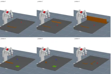
Fig. 2. In the 6 investigated problems the goal is to reach for the red ball or get the blue ball in the green area. Solutions involve using a hook to pull a desired object, push-sliding a ball along a wall, pushing a ball onto a strip of paper to then pull it closer, hitting a ball with a stick, throwing a box at a ball, and using a hook to reach for another hook to reach a ball.
problem 1 2 3 4 5 6
tree size 12916 34564 7312 12242 12242 3386 branching 10.66 13.63 9.25 10.52 10.52 7.63
Fig. 3. Size of decision trees of depth 4, and branching factor estimate (4th root). For problem 6 we had to limit the logic to exclude dynamic interactions, otherwise the tree size would have been 349252 with branching factor 24.31.
optimization convergence in the next section. The aim of explicitly modeling modes was to capture the multi-modal complexity of the overall manipulation planning problem. Convergence consistency of our bound evaluations is an in-dicator for how this modeling leaves a simpler structured problem for the conditional path optimization.
VI. EXPERIMENTS
The source code2 and a supplementary video3 for our
experiments are available for reference.
We investigated our method on 6 problems as illustrated and described in Fig. 2. The problems were designed to cover a spectrum of types of interactions, including the need to use tools, hit objects, or throw objects in order to reach the goal. The accompanying video illustrates the problems, and the source code includes the precise scene descriptions. The video displays the computed paths x, not a simulation of their execution. The solver surprised us in finding much larger varieties of solutions than anticipated. For instance, in problem 1 a natural solution is grasping the hook, pulling the ball, and grasping it. Our method also found solutions that involve hitting the ball, or sliding the hook to the ball to hit it. Handovers are much more frequent than anticipated. The solver exploited the combinatorics of manipulations that are possible with the given primitives beyond what we had in mind when designing the problems.
2https://github.com/MarcToussaint/18-RSS-PhysicalManipulation 3https://www.youtube.com/watch?v=-L4tCIGXKBE
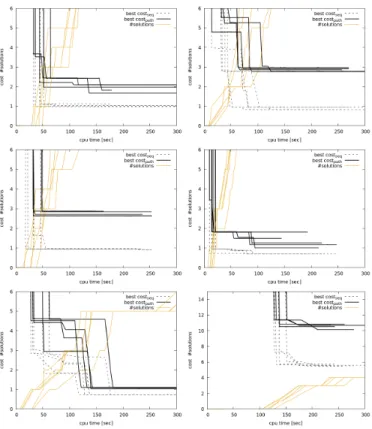
Fig. 4. For 5 runs for each problem we display cost of the best solution found, for boundsP2 (dotted) andP3(solid), over time.
To get an idea of the branching factor (which varies over the tree depth) Fig. 3 provides the tree size for skeletons of length 4 (3 is the minimum, most found solutions are of length 4-6). Clearly, cutting the tree search as proposed by MBTS is essential for efficient search in such trees.
The solver is an anytime method. For each problem we ran it until 12 solutions (with different skeletons) were found or 400 seconds were exceeded. The solver then presents and ranks solutions by their cost. Fig. 4 displays traces of runs for each problem, i.e., the cost of the best found solution over time, descending as a step function whenever a better solution is found, and the total number of solutions found. While the dotted line displays the cost of the lower bound P2 for the
best solution, the solid line displays the full path costs P3.
All runs reliably found solutions at around 50 seconds, except for problem 6. This problem is special in that it only affords one stereotypical solution: grasp first hook, pull second, grasp second, pull ball, grasp ball, and somewhere in between place a hook down to allow for the final grasp. The depth of this solution required around 150 seconds. The variance in the cost of the best solution found shows that not all optimizations converge to the global optimum (each Pi is non-convex).
Fig. 5 displays the mean run times of the Gauss-Newton methods for solving the bounds P1,P2,P3, where P3 is the
full path. We display these separating runs that turned out as feasible vs infeasible. The optimization times increase with the depth of the manipulation sequence, as well as with the
Fig. 5. Mean run times for the computation of the different bounds (solving P1,P2,P3), depending on feasibility and infeasibility.
bound level. Interestingly, especially for the coarse bounds P1 andP2, the run times are significantly shorter for feasible
solutions. This also holds for the full path optimizationP3, but
less so. A major part of the computation time is spent on trying to solve infeasible problems. Therefore, reliable indicators or classifiers to predict infeasibility earlier could significantly speed up the solver.
For problem 1 we investigated convergence consistency across 10 runs: whenever a specific skeleton was evaluated more than 5 times for a particular bound across all trials, we investigated whether the evaluations converged to consistent optima. Concerning bounds P1 and P2, we found 100%
consistency in terms of feasibility (all runs agreed on the feasi-ble/infeasible label for a skeleton) except for a single skeleton which boundP1 labeled feasible only 4 out of 5 times. The
corresponding cost estimates were equally consistent, with a mean variance of only 0.00133 for P1 and 0.0080 for P2
for a skeleton. The full path evaluation P3 converges less
consistently to the same optima. For 11 out of 24 skeletons the runs were 100% consistent with very low cost variance; for the remaining skeletons the consistency was mixed. This explains the variance of best solutions found in Fig. 4. Nevertheless, all runs consistently found good solutions.
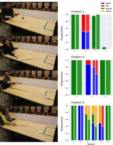
We also performed a study of 5 human subjects on problems analogous to our problems 1, 3, and 6, see Fig. 6. The right column displays frequencies of action primitives used along the skeleton for our method (solid) and the humans (striped). While we do not want to claim our method is a model for human decision making, it is interesting to compare to. In particular, we mention differences and limitations of our method in view of human execution. The first striking difference when watching the videos is the frequency of “re-initiations” of primitives executed by humans in a reactive manner, e.g. a frequent re-positioning of the tool to re-initiate pushing the same object. In the planned solutions, such re-initiations of the same interaction mode are largely missing as they would be considered sub-optimal. This underlines that our method only addresses a planning problem, rather than the problem of reactive and adaptive execution of such plans. Second, our method currently does not assume a fixed “true” friction coefficient between objects; instead, when the skeleton includes an inertial slide, the object slides nearly
friction-Problem 3 P roportions Problem 1 P roportions Problem 6 P roportions Steps
Fig. 6. 5 subjects were studied on 4 tasks analogous to our problems 1, 3, and 6 (where for problem 1 we tested also a high-friction puck replacing the ball).
less, and if the skeleton includes a push, the object resides stably at the pushing object. To solve problem 1, our method generates about equal numbers of solutions with inertial ball motions as well as with stable pushes. The human decisions depend on their perceptual estimate of the friction of the puck or ball. On problem 4, humans exploited the wall to slide along considerably more often than our algorithm. Our algorithm occasionally finds the slide-along-the-wall manip-ulation sequence (see video), it also finds shorter sequences that are preferred by the method but not by humans. Finally, especially in problem 5, the planner generates throw-box-to-hit-ball sequences that fulfill the impulse exchange equations but include extremely flat angles of impact (as in billiards), which are too precise for a human to accurately replicate. This shows a deficit of assuming deterministic physics for making such dynamic manipulation decisions.
VII. CONCLUSIONS
Our approach is, to our knowledge, the first to embed dy-namic physical manipulations in a TAMP framework, combin-ing a discrete logic level for sequences of possible interaction modes with a continuous path optimization level. We tackled sequential manipulation and tool-use planning problems, a
hallmark of intelligent behavior. While this work focuses on the technical formulation, it also serves as a foundation for future work on modeling animal and human behavior on such problems, which need to address the limitations discussed above.
We already mentioned several limitations when comparing to the human execution of manipulation tasks. We emphasize that the proposed method is only a planner, not a framework for executing such plans. As our method generates several alternative plans, reactive execution could leverage sample-efficient reinforcement learning mechanisms to select and switch between plans on the fly, depending on their success.
We believe that the predicates and logic rules of physical in-teractions can be reduced in future work to a more fundamental set, in particular by using a factored representation. This could address the inefficiencies we mentioned in the context of the hitSlideSit operator. We also note that the efficiency of the solver could be improved by combining LGP with more efficient AI planners [11, 9]. Particularly interesting is the idea in angelic semantics [18] to not only leverage lower bounds but also higher (pessimistic) bounds. Exploiting a hierarchy of bounds will remain crucial for efficiency. New bounds could be formulated specifically for physical reasoning, for instance an efficiently computable bound that only includes
touchconstraints — as this is a highly discriminative indicator of the feasibility of physical interactions.
ACKNOWLEDGMENTS
We thank Leslie Kaelbling and Tom´as Lozano-P´erez for the insightful discussions on TAMP. This work was partially supported by the Toyota Research Institute (TRI). However, this article solely reflects the opinions and conclusions of its authors and not TRI or any other Toyota entity. This work was also supported by the DFG under grant TO 409/9-1.
REFERENCES
[1] Samir Alili, A. Kumar Pandey, E. Akin Sisbot, and Rachid Alami. Interleaving symbolic and geometric reasoning for a robotic assistant. In ICAPS Workshop on Combining Action and Motion Planning, 2010. [2] Peter Battaglia, Jessica Hamrick, and Joshua B
Tenen-baum. Simulation as an engine of physical scene un-derstanding. Proceedings of the National Academy of Sciences, 110:18327–18332, 2013.
[3] Nikhil Chavan Dafle, Alberto Rodriguez, Robert Paolini, Bowei Tang, Siddhartha S. Srinivasa, Michael Erdmann, Matthew T. Mason, Ivan Lundberg, Harald Staab, and Thomas Fuhlbrigge. Extrinsic dexterity: In-hand manip-ulation with external forces. In Int. Conf. on Robotics and Automation (ICRA’14). IEEE, 2014.
[4] Lavindra de Silva, Amit Kumar Pandey, Mamoun Gharbi, and Rachid Alami. Towards combining HTN plan-ning and geometric task planplan-ning. arXiv preprint arXiv:1307.1482, 2013.
[5] Robin Deits and Russ Tedrake. Footstep planning on uneven terrain with mixed-integer convex optimization. In RAS Int. Conf. on Humanoid Robots. IEEE, 2014.
[6] Clemens Eppner, Raphael Deimel, Jos´e ´Alvarez-Ruiz, Marianne Maertens, and Oliver Brock. Exploitation of environmental constraints in human and robotic grasping. The International Journal of Robotics Research, 34: 1021–1038, 2015.
[7] Filipe de Avila Belbute-Peres and J. Zico Kolter. A Modular Differentiable Rigid Body Physics Engine. In Neural Information Processing Systems (NIPS’17), 2017. [8] Jason Fischer, John G Mikhael, Joshua B Tenenbaum, and Nancy Kanwisher. Functional neuroanatomy of intuitive physical inference. Proceedings of the national academy of sciences, 113:E5072–E5081, 2016.
[9] CR Garrett, T Lozano-Prez, and LP Kaelbling. STRIP-Stream: Integrating Symbolic Planners and Blackbox Samplers. e-Print arxiv.org:1802.08705, 2018.
[10] Kris Hauser and Jean-Claude Latombe. Multi-modal mo-tion planning in non-expansive spaces. The Internamo-tional Journal of Robotics Research, 29:897–915, 2010. [11] Leslie Pack Kaelbling and Tom´as Lozano-P´erez.
Hierar-chical task and motion planning in the now. In Int. Conf. on Robotics and Automation (ICRA’11), pages 1470– 1477. IEEE, 2011.
[12] Wolfgang K¨ohler. Intelligenzpr¨ufungen am Menschenaf-fen. Springer, Berlin (3rd edition, 1973), 1917. English version: Wolgang K¨ohler (1925): The Mentality of Apes. Harcourt & Brace, New York.
[13] Fabien Lagriffoul, Dimitar Dimitrov, Alessandro Saf-fiotti, and Lars Karlsson. Constraint propagation on inter-val bounds for dealing with geometric backtracking. In Int. Conf. on Intelligent Robots and Systems (IROS’12), pages 957–964. IEEE, 2012.
[14] Fabien Lagriffoul, Dimitar Dimitrov, Julien Bidot, Alessandro Saffiotti, and Lars Karlsson. Efficiently combining task and motion planning using geometric constraints. The International Journal of Robotics Re-search, 2014.
[15] Steven M. LaValle. Planning Algorithms. Cambridge university press, 2006.
[16] Tom´as Lozano-P´erez and Leslie Pack Kaelbling. A constraint-based method for solving sequential manip-ulation planning problems. In Int. Conf. on Intelligent Robots and Systems (IROS’14), pages 3684–3691. IEEE, 2014.
[17] Kevin M. Lynch and Matthew T. Mason. Stable pushing: Mechanics, controllability, and planning. The Interna-tional Journal of Robotics Research, 15:533–556, 1996. [18] Bhaskara Marthi, Stuart J. Russell, and Jason Andrew Wolfe. Angelic Semantics for High-Level Actions. In ICAPS, pages 232–239, 2007.
[19] Matthew Mason. The mechanics of manipulation. In Int. Conf. on Robotics and Automation (ICRA’85). IEEE, 1985.
[20] Matthew Moore and Jane Wilhelms. Collision detection and response for computer animation. In ACM Siggraph Computer Graphics, volume 22, pages 289–298. ACM, 1988.
[21] Igor Mordatch, Emanuel Todorov, and Zoran Popovi´c. Discovery of complex behaviors through contact-invariant optimization. ACM Transactions on Graphics (TOG), 31(4):43, 2012.
[22] Franc¸ois Osiurak and Arnaud Badets. Tool use and affordance: Manipulation-based versus reasoning-based approaches. Psychological Review, 123:534, 2016. [23] Michael Posa, Cecilia Cantu, and Russ Tedrake. A
direct method for trajectory optimization of rigid bodies through contact. The International Journal of Robotics Research, 33(1):69–81, 2014.
[24] David A Rosenbaum, Caroline M van Heugten, and Graham E Caldwell. From cognition to biomechanics and back: The end-state comfort effect and the middle-is-faster effect. Acta psychologica, 94:59–85, 1996. [25] Arne Sieverling, Clemens Eppner, Felix Wolff, and
Oliver Brock. Interleaving motion in contact and in free space for planning under uncertainty. In Int. Conf. on Intelligent Robots and Systems (IROS’17), pages 4011– 4073. IEEE, 2017.
[26] Thierry Sim´eon, Laumond Jean-Paul, Juan Cort´es, and Anis Sahbani. Manipulation Planning with Probabilistic Roadmaps. The International Journal of Robotics Re-search, 23:729–746, 2004.
[27] Siddharth Srivastava, Eugene Fang, Lorenzo Riano, Ro-han Chitnis, Stuart Russell, and Pieter Abbeel. Combined task and motion planning through an extensible planner-independent interface layer. In Int. Conf. on Robotics and Automation (ICRA’14), pages 639–646. IEEE, 2014. [28] Aviv Tamar, Yi Wu, Garrett Thomas, Sergey Levine, and Pieter Abbeel. Value iteration networks. In Advances in Neural Information Processing Systems, pages 2154– 2162, 2016.
[29] Emanuel Todorov. A convex, smooth and invertible contact model for trajectory optimization. In Int. Conf. on Robotics and Automation (ICRA’11), pages 1071–1076. IEEE, 2011.
[30] Emanuel Todorov, Tom Erez, and Yuval Tassa. MuJoCo: A physics engine for model-based control. In Int. Conf. on Intelligent Robots and Systems (IROS’12), pages 5026–5033. IEEE, 2012.
[31] Marc Toussaint. Logic-geometric programming: An optimization-based approach to combined task and mo-tion planning. In Proc. of the Int. Joint Conf. on Artificial Intelligence (IJCAI 2015), 2015.
[32] Marc Toussaint and Manuel Lopes. Multi-bound tree search for logic-geometric programming in cooperative manipulation domains. In Proc. of the IEEE Int. Conf. on Robotics and Automation (ICRA 2017), 2017. [33] Joanna H Wimpenny, Alex AS Weir, Lisa Clayton,
Christian Rutz, and Alex Kacelnik. Cognitive processes associated with sequential tool use in new caledonian crows. PLoS One, 4:e6471, 2009.
![Fig. 1. From left to right: A crow solving a sequential hook problem [33], classical intelligence test with apes [12], our solver using a stick to hit a flying blue ball to get it into the green area, using a hook to get a second hook to reach for the red](https://thumb-eu.123doks.com/thumbv2/123doknet/14746029.578196/2.918.470.846.315.779/solving-sequential-problem-classical-intelligence-solver-flying-second.webp)