HAL Id: hal-02380162
https://hal.archives-ouvertes.fr/hal-02380162
Submitted on 31 Mar 2021
HAL is a multi-disciplinary open access
archive for the deposit and dissemination of
sci-entific research documents, whether they are
pub-lished or not. The documents may come from
teaching and research institutions in France or
abroad, or from public or private research centers.
L’archive ouverte pluridisciplinaire HAL, est
destinée au dépôt et à la diffusion de documents
scientifiques de niveau recherche, publiés ou non,
émanant des établissements d’enseignement et de
recherche français ou étrangers, des laboratoires
publics ou privés.
Onland and Offshore Extrinsic Fabry–Pérot Optical
Seismometer at the End of a Long Fiber
Pascal Bernard, Romain Feron, Guy Plantier, Alexandre Nercessian, Julien
Couteau, Anthony Sourice, Mathieu Feuilloy, Michel Cattoen, Han-cheng
Seat, Patrick Chawah, et al.
To cite this version:
Pascal Bernard, Romain Feron, Guy Plantier, Alexandre Nercessian, Julien Couteau, et al.. Onland
and Offshore Extrinsic Fabry–Pérot Optical Seismometer at the End of a Long Fiber. Seismological
Research Letters, Seismological Society of America, 2019, 90 (6), pp.2205-2216. �10.1785/0220190049�.
�hal-02380162�
1
Seismological Research Letters
November 2019, Volume 90 Issue 6 Pages 2205-2216 https://doi.org/10.1785/0220190049
https://archimer.ifremer.fr/doc/00585/69743/
Archimer
https://archimer.ifremer.frOnland and Offshore Extrinsic Fabry–Pérot Optical
Seismometer at the End of a Long Fiber
Bernard Pascal 1, * , Feron Romain 2, 3, Plantier Guy 2, 3, Nercessian Alexandre 1, Couteau Julien 1,
Sourice Anthony 2, 3, Feuilloy Mathieu 2, 3, Cattoen Michel 4, Seat Han‐cheng 4, Chawah Patrick 5,
Chéry Jean 5, Brunet Christophe 1, Boudin Frédérick 6, Boyer Daniel 7, Gaffet Stéphane 7, Geli Louis 8,
Pelleau Pascal 8
1 IPGP, Université de Paris, UMR 7154 CNRS, 1 rue Jussieu, 75005 Paris, France 2 ESEO Group, 10 Boulevard Jean Jeanneteau, 49100 Angers, France
3 Also at LAUM, Université du Maine, Avenue Olivier Messiaen, 72085 Le Mans, France. 4 LAAS‐CNRS, 7 Avenue du Colonel Roche, 31400 Toulouse, France
5 Géosciences Montpellier, Place Eugène Bataillon, 34090 Montpellier, France 6 Département de Géologie, ENS Paris, 24 Rue Lhomond, 75005 Paris, France 7 Laboratoire Souterrain à Bas Bruit (LSBB), 84400 Rustrel, France
8 IFREMER, 1625 Route de Sainte‐Anne, 29280 Plouzané, France
* Corresponding author : Pascal Bernard, email address : bernard@ipgp.fr ; romain.feron@eseo.fr ; guy.plantier@eseo.fr ; nerces@ipgp.fr ; couteau@ipgp.fr ; anthony.sourice@sigfrance.com ; mathieu.feuilloy@eseo.fr ; michel.cattoen@laas.fr ; han.cheng.seat@laas.fr ; patrick.chawah@gmail.com ; jean.chery@gm.univ-montp2.fr ; brunet@ipgp.fr ; boudin@geologie.ens.fr ; daniel.boyer@lsbb.eu ; stephane.gaffet@lsbb.eu ; louis.geli@ifremer.fr ; pascal.pelleau@ifremer.fr
Abstract :
We report here the design, performance, and in situ demonstration, on‐land and offshore, of an innovative high‐resolution low‐cost optical (laser) seismometer. The instrument was developed within the Laser Interferometry for Earth Strain project (French Agence Nationale de la Recherche [ANR] program), and first tested at the low‐noise underground laboratory Laboratoire Souterrain à Bas Bruit (LSBB, France). It is based on Fabry–Pérot optical interferometry between the extremity of a probing optical fiber and a reflecting mirror secured to the mobile mass of a passive 2 Hz geophone. The detection technique is based on the wavelength modulation of the laser diode (1310 nm), which allows the separation of the optical power into two signals in quadrature, thanks to an heterodyne technique. The relative displacement of the mobile mass is retrieved in real time by the phase unwrapping of these two signals. At LSBB, the fiber was 3 km long. It recorded many teleseismic earthquakes and a few regional ones, and resolves the low‐seismic noise of the Earth for periods up to 6 s, presenting an acceleration noise floor lower than 1 ng/Hz−−−√ in the 0.3–5 Hz range. A three‐component version of this fiber‐based interferometric 2 Hz geophone has been recently constructed, shielded in a hyperbaric container, and installed offshore for test in Brittany (France) in April 2018, with an improved control system. Its record of the marine ambient noise matches those of a collocated commercial broadband seismometer for periods up to 50 s. This
2
opens promising perspectives for large‐scale ocean bottom instrumentation with up to 50‐kilometer‐long optical lines; an installation is planned for 2020, off Guadeloupe, with a 5‐kilometer‐long fiber cable. It may also prove useful for installations in other challenging and exposed environments, such as deep hot boreholes, active volcanoes, unstable landslides, for real‐time monitoring in regions with high natural hazard, but also for seismic monitoring of geoindustries.
Introduction
In many areas with high telluric hazard (earthquakes, tsunamis, landslides,..), our understanding of the seismogenic and mechanical processes, as well as our ability to properly assess the related hazard, are still very limited by the difficulty or impossibility to deploy arrays of high performance seismometers. This can be due to the high cost of the installations and of their maintaining, to the risk of loss (from lightning, eruptions, rock falls, power fail-ure...), or even to the lack of suitable commercial technology (high temperature). These difficulties are obvious for long term real-time seismic monitoring in the far offshore (in particular in the threatening subduction zones), in deep boreholes ( like the San Andreas Fault Observatory at Depth - SAFOD - on the San Andreas fault), or on active volcanoes. Similar difficulties are encountered in the geoindustry context of production, injection and storage (geothermy, oil, gas, deep mines, CO2and nuclear waste storage,..), which often requires seismic monitoring either offshore or in deep, hot boreholes.
Some of the difficulties above, together with the need for improving the resolution of commercial seismome-ters, have led a few academic and industrial groups to develop prototypes of optical seismometers. A fundamental interest of an opto-mechanical seismometer is the separation, by a long optical fiber, of the mechanical part of the sensor from the electro-optical part connected to the laser, photo-diodes, control cards, digitizer and PC. In addition, the long optical fiber is insensitive to electromagnetic perturbations, whether from lightning strikes, power lines, or industries. Furthermore, the mechanical part, requiring no electronic/electrical components, can therefore be robust and low cost. Also, the fiber and the mechanical sensor are much less sensitive to temperature than the commercial feed-back or inductive seismometers, allowing measurements in places where the latter sensors are rapidly damaged or cannot operate. Finally, the low cost of the mechanical sensor allows some installations at risk, for the sensor can be replaced if lost.
All these advantages should make a high resolution optical seismometer with long fibers much more suitable than commercial standard geophones (passive electro-magnetic, or force-balanced) in a broad frequency range 0.1 Hz to 10 kHz for many applications involving real-time monitoring.
In this paper, we present the design, performance and in situ demonstration of an innovative, high resolu-tion, low-cost optical (laser) seismometer. After a brief review of the progress in the field of optical seismometry over the last two decades, we present the design of our optical geophone, and the laboratory performance of the opto-electronic system. Next, we detail the installation of the instrument, first at the LSBB Observatory (South-ern France), second at the ESEO Group laboratory (West(South-ern France), and finally on the sea floor at the Sea Test Base, in Brittany, France. We finally present the resulting in situ performance, analyze the noise level, and
com-pare its records of large teleseismic earthquakes and small regional ones to those of nearby, reference broadband seismometers.
Development of high resolution laser seismometry
The emergence and rapid development of new technologies based on fiber optics offers a promising future in seis-mology. Several applications use back-scattering properties of the fiber itself, which is thus used as the sensor device (“intrinsic” sensors). The most classical intrinsic sensors are based on Fiber Bragg Grating (FBG), where some segments of the fiber are marked periodically to reflect a specific optical wavelength, allowing high accu-racy for measuring the local static or dynamic strain of the fiber (e.g., Bostick (2000), Keul et al. (2005)). Over the past decade, FBG coupled with a mechanical resonator has led to the development of more sophisticated op-tical seismometers (e.g., Huang et al. (2018)). In parallel, boosted by the oil and gas industry in the last decade, the “Distributed Acoustic Sensing” (DAS) technique has been developing very rapidly. DAS uses the Rayleigh backscattered light in standard (non grating) fibers, for recording the fiber dynamic strain induced by seismic vi-brations (Mestayer et al. (2011); Liu et al. (2017)). It has been tested for monitoring natural earthquakes (e.g., Lindsey et al. (2017); Wang et al. (2018); Jousset et al. (2018) ). Other techniques like laser reflectometry using BOTDR (Brillouin Optical Time Domain Reflectometry), for static strain measurements, are commonly used for the monitoring of engineering structures. The latter technique is presently tested during the FOCUS project to demon-strate the feasibility of measuring small (1-2 cm) displacements across an active fault off the coast of eastern Sicily (Dellong et al. (2018)). Finally, telecommunication optical fiber cables can detect seismic events when combined with state-of-the-art signal processing techniques (e.g., Marra et al. (2018)), but the related signals, being integrated overs tens to hundreds of kilometers of line, are far from being relevant for detailed source studies.
The alternative optical techniques to all these intrinsic fiber sensing approaches started 20 years ago (Chen et al. (1999)) , based on laser interferometry with small sensing cavities placed at the end of the optical fibers, hence de-signed as “extrinsic” interferometers. The Michelson and Fabry-Perot (FP) systems allow for very high resolution seismic recording. Zumberge et al. (2010) demonstrated the Michelson device on the spring-mass system of a long period STS1 seismometer, for observatory needs. They are currently working on borehole installations, improving its resolution, in particular in the long period range for broad band recordings (Zumberge et al. (2018)). A similar technique was used for a broad-band ocean borehole application (Araya et al. (2007)).
There are major differences between intrinsic and extrinsic sensing schemes. In DAS, the former can have a very high number (hundreds to thousands) of sensing points within a single fiber, interrogated by a single device, but
usually presents a much higher noise level, typically of a few nanostrain at best. The induced strain of the ground is of the order of the ground velocity divided by the wave velocity. Considering surface waves propagating typically at 3 km/s at a few seconds period, the smallest resolved ground velocity is typically 10−9∗ 3km/s (taking a strain noise floor of 1 nanostrain), hence of the order of 3 ∗ 10−6m/s. This leads to an acceleration noise floor larger than 5∗ 10−6m/s2. A similar value is obtained for higher frequencies, for instance considering surface waves at 3 Hz propagating at 300 m/s. This acceleration noise floor, of the order of 1 micro-g or more, is much larger than the few nano-g resolved by geophones.
Also, DAS systems may present poorly known effective transfer function from ground motion, due to the uncontrolled coupling of the fiber to the ground. Most seismometers do not suffer such problem, thanks to the usually carefull installation of each sensor on a concrete basis, well anchored on stable ground. Such an effort is not usually done for every meter along a pluri-kilometric optical cable. Thus, DAS systems provide new but fuzzy information on seismic sources, still difficult to interpret in terms of magnitude, mechanism, and spectral content.
The DAS system also requires a relatively high power supply (200-400 W), unsuitable for some observatories with remote installations. Conversely, extrinsic interferometry typically requires one fiber per sensor for FP (two fibers per sensor for Michelson devices), but a much higher resolution (down to a few nano-g rms in the 1-10 Hz range), and a well defined transfer function for the 3 components of ground displacement, allowing all the advanced processing and analysis in source seismology – and comparatively much lower power needs (for a small number of sensors).
To briefly summarize, we note that although various models of optical seismometers have been developed by a few academic institutions and by some companies in the last two decades, a simple, low-cost, low-power, medium band (1 Hz-1 kHz), high resolution, and long (plurikilometric) fiber-based optical equipment has not yet been pro-posed by the geophysical sensor industry.
Because of its high resolution, qualified calibration, long range capabilities, and low power need, the FP in-terferometry technique has been selected for R & D by IPGP more than a decade ago. In 2007, inspired by the first promising results with extrinsic interferometry applied for optical seismometry, pioneered by Zumberge et al. (2003), we started to develop our own opto-mechanical system, however with a different goal than broad-band seis-mology : we rather targeted the design of short-period geophones, plugged at the end of plurikilometric optical lines, for seismological and volcanic Observatories worldwide. The latter have indeed a clear need of such instruments for deep borehole, far offshore, mountainous/volcanic, and antennae installations, in challenging environments. This was the initial motivation of our LINES project.
Design of the LINES seismometer prototype
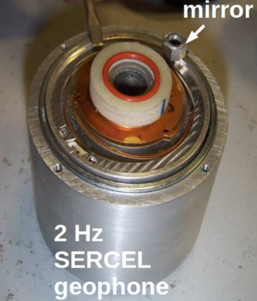
In 2007-2008, using a simple horizontal 2 Hz geophone modified by the addition of a small mirror fixed on its mobile mass, preliminary tests were performed at the OSE research group of LAAS-CNRS (OSE-LAAS) in Toulouse. The interrogating laser beam was pointed at the mirror, for measuring, with Fabry-Perot (FP) interferometry, the displacement of the mass relative to the main frame fixed to the ground and holding the end of the optic fiber.
The encouraging results led us to develop further the whole system within the LINES ANR project (2009-2012) (Chawah (2012); Chawah et al. (2012); Chery et al. (2012); Seat et al. (2012)). Two other optical instruments were also designed and constructed within the LINES project: a borehole tiltmeter, and a long base hydrostatic tiltmeter. All three instruments were successfully demonstrated in a test tunnel at the Laboratoire Souterrain à Bas Bruit (LSBB, low background noise underground laboratory) in Rustrel, southern France (Chery et al. (2012)). The main partners of LINES were Geoscience Montpellier, coordinating the LINES project, and developing the mechanical part of the tiltmeters, IPGP, for the optical adaptation of the seismometer, OSE-LAAS in Toulouse, for the opto-electronic and fiber sensor developments, and ESEO in Angers, for the new algorithms for processing of the optical signal.
Geophone
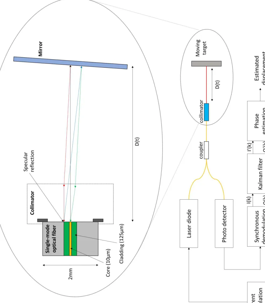
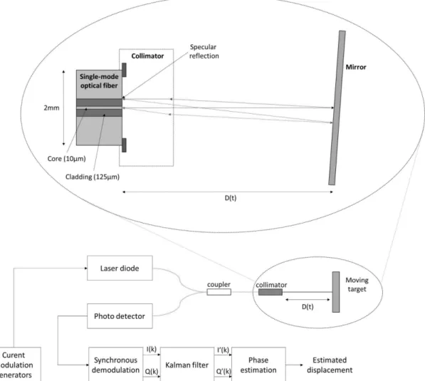
The LINES seismometer is based on a FP optical interference, in the fiber, between the reference beam reflected at the end of the fiber, and the probe beam reflected on the mirror set on the mobile mass of a geophone (Bernard et al. (2017) ). It thus differs from Zumberge’s (2011) instruments, which use Michelson interferometry and therefore require 2 optical fibers per sensor, instead of one for FP.
For the passive geophone, we selected a horizontal L22 Sercel, 2 Hz, based on the high mechanical stability, linearity, and reliability of this commercial geophone, as well as on the relatively easy operation for integrating the mirror.
The latter operation was done by : (1), removing the metallic cylindrical housing of the geophone fixing an optical mirror (mass 10 g, diameter 3 mm) on the external face of the mobile coil; (2) cutting off the metallic top of the cylindrical housing, on the mirror side, and replacing it by a custom cap allowing space for the mirror to move without touching the new cap; and (3) opening a hole in the cap for allowing the laser beam from the external collimator to reach and reflects freely (through air) on the internal mirror. The insertion of the mirror on the mobile coil mass changed the mass balance, resulting in a resonance frequency shift from 2 to 2.4 Hz (figure 1).
Optics
The control and recording system is set at the other end of the optic fiber. It includes a laser diode at 1310 nm for the source, and a photo diode for the receiver, controlled by a signal processing unit (figure 2). The choice of the 1310 nm wavelength was made because it provides a small attenuation with distance (about 0.4 dB/km) , and because it is a very common commercial standard with rather low-cost associated equipment.
The distance of the target D(t) and the instantaneous wavelength λ(t) induces a phase difference Φ(t) between the reference (emitted) wave and the sensing wave (n is the media index).
Φ(t) = 4πn· D(t)
λ(t) (1)
The photodiode signal s(t), proportional to the power of the wave, can be simply described by the following equation:
s(t) = A(t)· cos(Φ(t)) (2)
A simple sinusoidal modulation F m1of the laser diode current involves an amplitude modulation A(t) of the interferometric signal - directly proportional to the current - and the modulation of the laser’s wavelength λ(t).
s(t) = A(t)· cos(4πn ·D(t)
λ(t) + m1(t)), (3)
where m1is the phase shift resulting from the F m1modulation.
We demonstrated that a synchronous quadrature demodulation - which allows to extract 2 intensity signals in approximate quadrature I(t) and Q(t) (equations 4 and 5) - coupled with fast and innovative real-time algorithms for instantaneous phase estimation, makes it possible to estimate the displacement of the target (Chawah et al. (2011)). I(t) = AI(t)· cos(4πn · D(t) λ(t)) + BI(t) (4) Q(t) = AQ(t)· cos(4πn · D(t) λ(t) + α) + BQ(t) (5)
In fact, when the displacement D(t) varies, a plot of Q(t) as a function of I(t) describes an elliptic curves with time varying parameters : BI(t),BQ(t)the center of the ellipse, AI(t),AQ(t) the amplitudes and α(t) the orientation (due to the phase shift between I(t) and Q(t)). These 5 parameters have to be jointly estimated in addition to the distance D(t). This operation is performed by a real-time Kalman filter.
However, the real time quadrature demodulation will erase the phase information if there is no displacement. Indeed, in this case, the estimated phase difference remains constant. In order to ensure that the following estimation algorithms work properly, we need to introduce a redundant information in the emitted signal that we can consider as a virtual displacement. This information is included in a second modulation F m2of the laser diode signal.
s(t) = A(t)· cos(4πn ·D(t)
λ(t) + m1(t) + m2(t)) (6)
where m2is the phase shift resulting from the F m2modulation.
At first, we choose a 50 kHz modulation frequency for F m2, and a 1 kHz modulation frequency for F m1. After a complete mounting of the optical/recording system, we analyzed its noise level by replacing the mobile mirror of the geophone by a fixed one, keeping a stable length of the laser cavity (between the mirror and the collimator at the extremity of the fiber). A 13 days long testing period showed that the distance noise has a typical RMS value of 64 pm in the 2 mHz-100 mHz frequency band, and 124 pm in the broader 1 mHz-50 Hz frequency band, and that the velocity RMS noise is 12 pm/s in the 2 mHz-100 mHz range.
The dynamic range of the sensor is limited in relative displacement by the mechanical stop for the mass (5 mm in our prototypes), and in relative velocity by the capability to properly sample the optical fringes in real time. A correct unwrapping of the phase indeed requires to have enough measurement points while the optical path is changing by one wavelength. Given the sampling rate of the photodiodes (50 KHz), the wavelength (1310 nm), and the double reflection on the mirror, one gets a velocity cutoff of about 2 mm/s, above which the (I,Q) ellipses are not sampled well enough for an accurate calculation of the mass displacement. To summarize, for the displacement (resp. velocity), with a noise floor of 64 pm (resp. 12 pm/s) and a maximum of 5 mm (resp. 2 mm/s), the dynamic range is about 26 bits (resp. 28 bits).
Underground installation at LSBB
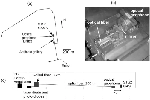
The LSBB site has been selected for setting the global LINES experiment, because of its mechanically and ther-mally stable underground environment ( http://www.lsbb.eu), mostly requested for the tiltmeters. In addition, the seismometer installation of LINES (referred to as SL hereafter) benefitted from the existing broadband seismome-ter array of LSBB. The horizontal optical geophone has been installed on the floor of a small room near the end of the long “antiblast” tunnel, with 300 m of overburden, about 900 m away from the main entrance (figure 4). It is fixed on a rigid metallic platform which also supports the collimator, and oriented North. The distance between the latter and the mobile mirror is set to 1 cm. The whole system is covered by a rigid box with Plexiglas walls, fixed and sealed onto the metallic horizontal platform, aiming at creating a humidity proof protection for the geophone. Indeed, the latter is highly sensitive to atmospheric humidity which oxydates its metallic components, owing to the
open hole letting the external laser beam reach the mirror of the mobile mass.
The closest broadband seismometer of the LSBB array, GAS, is an STS2 sensor (120 s) located in the neigh-bouring room, at the end of the tunnel, about 7 m away. In the following we analyze the records at 20 Hz sampling rate, high enough for calibrating and qualifying the optical sensor both at higher and lower frequencies than its resonance – with more emphasis on its ability to record the lowest frequencies. The optical geophone at LSBB was connected to the end of a 3 km long optical, monomode fiber. The latter is mostly rolled, as only 300 m of a straight tunnel separates SL from the operating room where the control/recording system was installed.
To calibrate the geophone, we used the parametrized representation of its transfer function, assuming a one degree of freedom oscillator with 2 unknowns: damping, and resonant frequency. These parameters were adjusted with the known input displacement of some earthquake inferred from the corresponding records by the North component of the GAS station. However, we observed some slow changes of the transfer function with time, and the seismometer finally got locked; after inspection, we found that despite the protection box, rust had developed on some of the springs, changing mass distribution, elasticity, and damping of the system in an unpredictable way - and finally blocking the whole coil. Therefore, the instrument calibration was done on records mainly corresponding to early observation times.
Offshore installation at STB
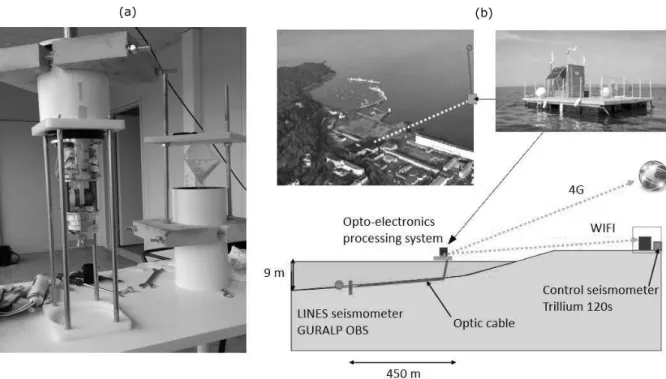
Based on the LINES prototype, we constructed a 3-component optical seismometer using 2 horizontals and 1 ver-tical 2 Hz Sercel geophones, aiming at offshore installations. Following standard constructions for short period offshore instruments, we mounted them in a rigid block, suspended with gimbals within a hyperbaric, duralumin casing, able to stand 300 MPa for offshore installations. A 2 cm thick layer of high viscousity oil was poured into the chamber, at the bottom of the sensor block, which allows for post-installation, passive self-leveling of the system with no need of power nor control. We added a fourth optical component inside the container, pointing to a fixed mirror, allowing for the measure of the self-noise (figure 5 - Left).
Meanwhile, before the offshore installation, we improved the performance of our system, in terms of instrumen-tation noise, signal processing, and power consumption. In order to validate these improvements, we conducted the next measurements at ESEO Group, Angers (France). Sensors were installed on a partially buried concrete slab in the basement of the building for several months. The manufactured sensors chosen for this campaign were the Guralp CMG-3ESP and a TRILLIUM compact 120s. During this period, sensors recorded the seismic noise,
allow-ing us to confirm the performance of our seismometer, and also many earthquakes such as the M7.1, 2017 Mexico earthquake and regional earthquakes.
The offshore test site was selected at the Sea Test Base (STB) of Lanveoc, in Brittany, France. This choice was primarily motivated by the proximity of IFREMER Brest for the installation and maintaining logistics, and by the facilities (power, telemetry, offshore platform with shelter, land-based shelter) and safety offered by STB. The offshore surface platform is anchored 1 km away from the coast, at 6m in depth (figure 5 - Right). The seismometer was installed by divers from IFREMER, embedded in about 60 cm of sand and shell debris, about 450 m north to the platform, at the depth of 9 m. A 500 m long optical cable connects the platform to the sensor, laying on the sea floor and secured every 20 m on screw anchors. Beneath the platform, the cable has a large slack in order to accommodate for the tide (max ±3m). Furthermore, the signal processing unit has been redesigned to reduce the power consumption, and to improve its robustness and reliability. Indeed, this new version of the instrumentation system consumes less than 30 W, to be compared with the 300 W of the LINES system running at LSSB on "on the shelve" commercial systems.
Results
At LSBB, we analyzed the instrumental noise of the control system by tipping the metallic platform by some 15 degrees, so that the geophone mass remains clipped and immobile with respect to the collimator. The power was calculated by stacking and averaging power spectral densities calculated over 10 time windows about an hour long. The resulting “floor noise” power spectrum is presented in Figure 6.
It shows that the noise level is close to the new low noise model (NLNM) in the range 0.2 to 3 Hz: it is below 1 ng/√Hzin the 0.3-5Hz range, and remains below 10 ng/√Hzin the 0.15-20 Hz range. The V-shape of the noise spectrum is the direct consequence of the correction of the mechanical transfer function (simple oscillator) applied to the optical record displacement noise. The increase of the noise level at high frequencies is thus due to the optical measurement, which tracks the displacement of the mass: the rather white noise in this measurement is thus multiplied by the square of the frequency when looking at the acceleration spectrum. Although there is no sharp cutoff in the acceleration response, the bandwidth may be considered to be limited to about a few mHz at low frequencies, and to hundreds of Hz at high frequencies (we successfully tested the instruments at 1 KHz in real-time).
With the geophone in operating mode (horizontal), in the absence of significant earthquakes, the daily stacked spectrum shows a seismic noise contribution above the floor noise between 0.15 Hz and 5 Hz. The corresponding time records are identical to those of the nearby STS2.
The seismometer ran with some interruption for more than two years at 100 Hz (2012-2014) , recording many large teleseismic earthquakes and some small regional ones - and tested successfully for a few months at 1 kHz after mid 2014 . Here we present two examples of such records.
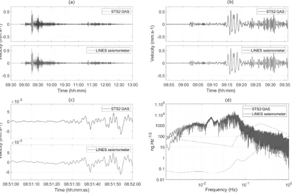
First, to illustrate the broad-band capabilities of this short-period mechanical sensor, we present and compare the records of SL and of GAS for the M=8.7, Sumatra 2012 earthquake, corrected for instrumental response and filtered in various frequency bands (Figure 7). Looking first at the 30 s time window around the P arrival, in the 0.2-10 Hz range (Fig. 7, bottom left), one clearly see the waveform matching of both instruments, even before the P wave arrival, hence for the background microseismic noise. Now, with a broader frequency range of 0.01 to 10 Hz, and focusing on the dominant surface waves, with period of 30 s, both records remain very similar (Fig. 7, top right). The last seismogram (Fig. 7, top left) shows 40 minutes of ground displacement inferred from both instruments, with again very similar waveforms. In the 0.01 Hz-1 Hz frequency range, after the corrections for the transfer function and for a slight miss-orientation of the optical geophone, the rms difference between the optical record and the STS2 record is less than 1.5%. Finally, the comparison of both spectra, for the same 2 hours long time window (Fig. 7, bottom right), shows that the 2 Hz geophone retrieved correct information from this energetic source at periods as long as 250 s.
This recovery of the lowest frequencies would be very challenging for an electrical geophone, as the latter measures the relative velocity of the mass (by induction), and not its relative displacement as does our FP-based geophone: the latter is intrinsically a lower frequency sensor.
The second example, in Figure 8, illustrates the higher frequency response of our sensor, with a regional earth-quake, 2015, M=3.4, which occurred 100 km away from LSBB. After correction from instrumental responses, both displacement records show a very strong similarity in the 0.1-20 Hz range.
The offshore experiment at STB showed a much larger noise level than at LSBB, resulting from the marine environmental noise, due to the swell 10 m above and to wave breaks at the coast line 1.5 km away. The noise floor , however, is slightly lower than for LSBB, due to the improvement of the new recording system produced by ESEO. To illustrate the quality of seismic records, we present those of the submarine mine blast, dated 05 April 2017 (Figure 9), and a teleseismic earthquake in Ionian Sea, M=6.8, 25 October 2018 (Figure 10), together with the corresponding GURALP records. For this large earthquake, the optical seismometer provides a good record up 50 s period, matching the Guralp waveform. Also, one notes in the bottom left part of the Figure that the background microseismic noise record of the Guralp, before the P wave arrival, is well matched by the optical seismometer, in
the dominant period range 2 to 5 s, with amplitude of a few 10−6m/s.
The performance of our passive, optical geophone can also be compared to the few best commercial seis-mometers involving optical measurements. The latter are however force-balanced, and their optical device is set for feed-back control. They are powered, the optoelectonic system is attached to the sensor and cannot operate remotely, as for example the Silicon Audio seismometer (http://www.siaudio.com/). Compared to the latter, our op-tical geophone reaches the same noise floor in the range 0.5-4Hz, but the absence of feedback increases its noise at lower and higher frequencies with respect to the force-balanced instrument. This is is an unavoidable consequence of a long fiber, purely optical measurement.
In addition to the instrumental noise floor, one might consider the transient optical noise produced within the fiber by the strain related to seismic waves, which might alter the optical FP signal from the sensor. For the LSBB experiment, which should have been the most sensitive experiment for such an effect (3 km long fiber), the seismic strain from regional nor teleseismic events did not seem to strongly impact the measurement: the related noise is indeed necessarely smaller than the difference in the records of the STS2 and the optical seismometer, and likely to be much smaller. Indeed, our FP measurement deals with the interference, within a single fiber, of the two reflected beams: to the first order, any strain-induced change in the optical path in this fiber (due to some shaking along the fiber) should affect both beams in the same way, and hence cancel our their effect on the phase pattern of their interference. Note that this cancelling might not be as good for extrinsic interferometry using Michelson principle, as the latter uses two optical fibers for a single measurement, one fiber carrying the reference beam.
Conclusion
We have constructed and qualified in situ, on-land and offshore, the prototype of a simple, high frequency opto-mechanical seismometer based on a 2 Hz geophone, to be cabled on long, plurikilometric optical fibers. The optical measurement of the displacement of the mobile mass of the geophone, by Fabry-Perot interferometry, allows to resolve the low noise level of the Earth at periods down to 5 s. This performance is due to the innovative design of real-time algorithms which processes the double modulation signal of the laser frequency. The system presents a floor noise of 1 ng/Hz1/2in the 0.5-5Hz range, remaining below 10 ng/Hz1/2in the 0.15-20 Hz range. Records of large (M8) teleseismic events show exploitable signals up to 250 s period, with a fidelity higher than 98.5% in the 10 mHz−1Hz range, as controlled by a nearby STS2. Thus, despite the high frequency character of the geophone, we obtained excellent results, significantly broadening the frequency range of a commercial 2 Hz geophone up to about 5 s periods ; a performance which is challenging for commercial inductive 2 Hz geophones on plurikilometric cables without amplifiers near the sensor. Also, for offshore installations, as shown at STB, because of the higher seismic noise level than on land, the performance of our optical sensor should allow to resolve seismic periods up to
several tens of seconds, and thus in particular contribute to the analysis of the sources of the primary and secondary microseismic waves.
As it is, our prototype can be used for marine or terrestrial applications, taking advantage of long optic cables (the SL was recently successfully tested on a 15 km long optic fiber, and is expected to operate with up to 50 km long fibers), to install the sensor in isolated, remote sites with difficult access, energy, and telemetry : this can be far offshore, on high mountains or volcanoes where eruptive activity, snow covering, and/or lightning does not allow for standard installations, and in deep, possibly hot boreholes. In this perspective, in the frame of the PREST project of the EC Interreg-Caraïbe program, the 3 component optical seismometer will be moved from Lanveoc to be installed 5 km offshore les Saintes islands (Guadeloupe), at 40 m in depth, connected to land by an optical cable. It will monitor in real-time the yet poorly resolved shallow microseismic swarms still occurring in the offshore source area of the M6.3, 2004 Les Saintes destructive earthquake. Miniaturization and simplification of the geophone is our next target of development, to allow for more applications, in particular for deep, slim and/or hot boreholes, and multi-sensor seismic antennas. Based on the same opto-electronics and control system, but using mechanical oscillators with much higher eigen-frequency, we also plan to develop strong motion accelerometers and hydrophones, which will enlarge the range of possible applications for this new optical instrument.
Data and Resources
The records of the STS2 VBB seismometer GAS from the Laboratoire Souterrain à Bas Bruit (LSBB) was made accessible through the open LSBB data base.
Acknowledgments
This study was supported by the Agence Nationale de la Recherche (ANR), France ("LINES" project, 2009-2012; "HIPERSIS" project, 2017-2018), by SATT OUEST-valorisation, France ( "SISMO MARIN" project ), by the LSBB underground research infrastructure, and the ISEN offshore research platform. The HIPERSIS project was certified by the Pôle AVENIA before submission to the ANR call. We particularly thank the divers from IFREMER, who installed the optical geophone offshore, and Didier Munck, Yves Auffret, and the STB team, for their logistic help at STB. We thank the Associate Editor and the two anonymous reviewers for their constructive comments.
References
Araya, A., K. Sekiya, and Y. Shindo, 2007. Laser-interferometric broadband seismometer for ocean borehole observations. In 2007 Symposium on Underwater Technology and Workshop on Scientific Use of Submarine Cables and Related Technologies. IEEE.
Bernard, P., C. Brunet, A. Nercessian, A. Sourice, M. Feuilloy, R. Feron, M. Cattoen, H.-C. Seat, P. Chawah, J. Chery, F. Boudin, D. Boyer, and S. Gaffet, 2017. The lines high resolution optical seismometer. In EAGE/DGG 2017 conference paper.
Bostick, F. X. T., 2000. Field experimental results of three-component fiber-optic seismic sensors. In SEG Technical Program Expanded Abstracts 2000. Society of Exploration Geophysicists.
Chawah, P., 2012. Developpement d’un capteur de déplacement à fibre optique applique à l’inclinometrie et à la sismologie. phdthesis, Université de Montpellier 2.
Chawah, P., A. Sourice, G. Plantier, and J. Chery, 2011. Real time and adaptive kalman filter for joint nanomet-ric displacement estimation, parameters tracking and drift correction of EFFPI sensor systems. In 2011 IEEE SENSORS Proceedings. IEEE.
Chawah, P., A. Sourice, G. Plantier, H.-C. Seat, F. Boudin, J. Chery, M. Cattoen, P. Bernard, C. Brunet, S. Gaffet, and D. Boyer, 2012. Amplitude and phase drift correction of efpi sensor systems using both adaptive kalman filter and temperature compensation for nanometric displacement estimation. Journal of Lightwave Technology, 30(13):2195–2202.
Chen, C., D. Zhang, G. Din, and Y. Cui, 1999. Broadband michelson fiber-optic accelerometer. Applied Optics, 38(4):628–30.
Chery, J., F. Boudin, H.-C. Seat, M. Cattoen, P. Chawah, G. Plantier, A. Sourice, P. Bernard, C. Brunet, S. Gaffet, and D. Boyer, 2012. Detecting aseismic transient motion on faults using new optical tiltmeters and seismometers. In AGU Fall Meeting.
Dellong, D., F. Klingelhoefer, H. Kopp, D. Graindorge, L. Margheriti, M. Moretti, S. Murphy, and M.-A. Gutscher, 2018. Crustal structure of the ionian basin and eastern sicily margin: Results from a wide-angle seismic survey. Journal of Geophysical Research: Solid Earth, 123(3):2090–2114.
Huang, W., W. Zhang, Y. Luo, L. Li, W. Liu, and F. Li, 2018. Broadband fbg resonator seismometer: principle, key technique, self-noise, and seismic response analysis. Opt. Express, 26(8):10705–10715.
Jousset, P., T. Reinsch, T. Ryberg, H. Blanck, A. Clarke, R. Aghayev, G. Hersir, J. Henninges, M. Weber, and C. Krawczyk, 2018. Dynamic strain determination using fibre-optic cables allows imaging of seismological and structural features. Nature Communications, 9:2041–1723.
Keul, P. R., E. Mastin, J. Blanco, M. Maguérez, T. Bostick, and S. Knudsen, 2005. Using a fiber-optic seismic array for well monitoring. The Leading Edge, 24(1):68–70.
Lindsey, N., E. Martin, D. Dreger, B. Freifeld, S. Cole, S. James, B. Biondi, and J. Ajo-Franklin., 2017. Fiber-optic network observations of earthquake wavefields. Geophysical Research Letters, 44(23):11,792–11,799.
Liu, X., C. Wang, Y. Shang, C. Wang, W. Zhao, G. Peng, and H. Wang, 2017. Distributed acoustic sensing with michelson interferometer demodulation. Photonic Sensors, 7(3):193–198.
Marra, G., C. Clivati, R. Luckett, A. Tampellini, J. Kronjäger, L. Wright, A. Mura, F. Levi, S. Robinson, A. Xuere, B. Baptie, and D. Calonico, 2018. Ultrastable laser interferometry for earthquake detection with terrestrial and submarine cables. Science, 361(6401):486–490.
Mestayer, J., B. Cox, P. Wills, D. Kiyashchenko, J. Lopez, M. Costello, S. Bourne, G. Ugueto, R. Lupton, G. Solano, D. Hill, and A. Lewis, 2011. Field trials of distributed acoustic sensing for geophysical monitoring. In SEG Technical Program Expanded Abstracts 2011. Society of Exploration Geophysicists.
Peterson, J., 1993. Observations and modeling of seismic background noise. Technical report, Open-File report 93-322, U.S. Geological Survey.
Seat, H.-C., P. Chawah, M. Cattoen, A. Sourice, G. Plantier, F. Boudin, J. Chéry, C. Brunet, P. Bernard, and M. Suleiman, 2012. Dual-modulation fiber fabry-perot interferometer with double reflection for slowly-varying displacements. Opt. Lett., vol. 37, no. 14, pp. 2886-2888.
Wang, H., X. Zeng, D. Miller, D. Fratta, K. Feigl, C. Thurber, and R. Mellors, 2018. Ground motion response to an ml 4.3 earthquake using co-located distributed acoustic sensing and seismometer arrays. Geophysical Journal International, 213:2020–2036.
Zumberge, M., J. Berger, W. Hatfield, and E. Wielandt, 2018. A three-component borehole optical seismic and geodetic sensor. Bull. Seismol. Soc. Am., 108(4):2022–2031.
Zumberge, M., J. Berger, J. Otero, and E. Wielandt, 2010. An optical seismometer without force feedback. Bulletin of the Seismological Society of America, 100(2):598–605.
Zumberge, M., J. Berger, and E. Wielandt, 2003. Experiments With an Optical Seismometer. AGU Fall Meeting Abstracts, Pp. S52C–0144.
Author’s mailing adress
• P. Bernard : bernard@ipgp.fr • R. Feron : romain.feron@eseo.fr • G. Plantier : guy.plantier@eseo.fr • A. Nercessian : nerces@ipgp.fr • J. Couteau : couteau@ipgp.fr • A. Sourice : anthony.sourice@sigfrance.com • M. Feuilloy : mathieu.feuilloy@eseo.fr • M. Cattoen : michel.cattoen@laas.fr • H.C. Seat : han.cheng.seat@laas.fr • P. Chawah : patrick.chawah@gmail.com • J. Chéry : jean.chery@gm.univ-montp2.fr • C. Brunet : brunet@ipgp.fr • F. Boudin : boudin@geologie.ens.fr • D. Boyer : daniel.boyer@lsbb.eu • S. Gaffet : stephane.gaffet@lsbb.eu • L. Geli : louis.geli@ifremer.fr • P. Pelleau : pascal.pelleau@ifremer.frList of Figures
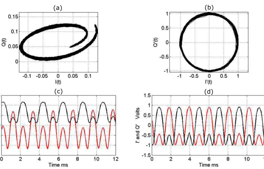
1 Opto-mechanical sensor. . . 18 2 Fiber-Optic Extrinsic Fabry-Perot Interferometer principle and processing scheme. . . 19 3 Effect of the Kalman Filter. (a) Lissajous plot of experimental (I(k),Q(k)) showing a spiral shape
caused by intensity modulation of the Laser Diode (left) and (b) corresponding circular Lissajous plot given by the Kalman filter (right). (c) Sampled signals I(k) and Q(k) (left) and (d) corrected quadrature signals I�(k)and Q�(k)(right). . . 20 4 Installation at LSBB. (a) General map view of LSBB - GAS is the STS2 (7m from the optical
sensor). (b) Optical geophone installation. (c) General installation of the opto-mechanical system . . 20 5 Installation test of the 3 component ocean bottom optical seismometer. (a) The 3 components
optical sensor. The 3 geophones to the left are suspended from the top of the hyperbar container. The bottom of the hyperbar container to the right is been filled with viscous oil (transparent in plastic bag), just before installation. (b) Pictures and schemes of the installation. . . 21 6 Acceleration noise curves. (a) 1 day PSD recorded at LSBB of the 2.4 Hz optical seismometer
LINES on a 3 km long fiber (solid curve) and STS2 GAS (dashed curve). (b) Measured Noise floor for LINES 2.4 Hz (clamped mass). Black solid curves : New Low Noise Model and New High Noise Model (Peterson (1993)). . . 21 7 Records of the Mw=8.7, 2012 Sumatra earthquake on the optical LINES seismometer and GAS at
LSBB. Horizontal ground velocity (a) and 40 minutes of horizontal ground velocity showing the dominant surface waves (b). 60s of horizontal ground velocity at LSBB near the P arrival time (c) and acceleration spectra (d). Black dashed curves : New Low Noise Model and New High Noise Model (Peterson (1993)). . . 22 8 Velocity records for a regional M=3.5 earthquake (2013, d=100 km). Filtered between 0.1 and 20 Hz. 22 9 Velocity record of the underwater blast in Brest bay of April 5, 2018. Data filtered in range [0.5 15]
Hz. LINES: Optical seismometer. . . 23 10 Records of the Mw=6.8, October 2018 Ionian Sea teleseismic earthquake. Data filtered in range
[0.02 2] Hz. Horizontal ground velocity (a) and 30 minutes of horizontal ground velocity showing the dominant surface waves (b). 60s of horizontal ground velocity near the P arrival time (c) and acceleration spectra (d). Black dashed curves : New Low Noise Model and New High Noise Model (Peterson (1993)). . . 24
Figure 3: Effect of the Kalman Filter.
(a) Lissajous plot of experimental (I(k),Q(k)) showing a spiral shape caused by intensity modulation of the Laser Diode (left) and (b) corresponding circular Lissajous plot given by the Kalman filter (right).
(c) Sampled signals I(k) and Q(k) (left) and (d) corrected quadrature signals I�(k)and Q�(k)(right).
Figure 4: Installation at LSBB.
(a) General map view of LSBB - GAS is the STS2 (7m from the optical sensor). (b) Optical geophone installation.
Figure 5: Installation test of the 3 component ocean bottom optical seismometer.
(a) The 3 components optical sensor. The 3 geophones to the left are suspended from the top of the hyperbar container. The bottom of the hyperbar container to the right is been filled with viscous oil (transparent in plastic bag), just before installation.
(b) Pictures and schemes of the installation.
Figure 6: Acceleration noise curves.
(a) 1 day PSD recorded at LSBB of the 2.4 Hz optical seismometer LINES on a 3 km long fiber (solid curve) and STS2 GAS (dashed curve).
(b) Measured Noise floor for LINES 2.4 Hz (clamped mass).
Figure 7: Records of the Mw=8.7, 2012 Sumatra earthquake on the optical LINES seismometer and GAS at LSBB.
Horizontal ground velocity (a) and 40 minutes of horizontal ground velocity showing the dominant surface waves (b). 60s of horizontal ground velocity at LSBB near the P arrival time (c) and acceleration spectra (d). Black dashed curves : New Low Noise Model and New High Noise Model (Peterson (1993)).
Figure 9: Velocity record of the underwater blast in Brest bay of April 5, 2018. Data filtered in range [0.5 15] Hz. LINES: Optical seismometer.
-0.2 0 0.2 Guralp 23:00 23:15 23:30 23:45 Time (hh:mm) -0.2 0 0.2 Velocity (mm.s -1) LINES seismometer -0.2 0 0.2 Guralp 23:10 23:15 23:20 Time (hh:mm) -0.2 0 0.2 Velocity (mm.s -1) LINES seismometer -0.02 0 0.02 Guralp 22:59:00 22:59:10 22:59:20 22:59:30 22:59:40 22:59:50 23:00:00 Time (hh:mm:ss) -0.02 0 0.02 Velocity (mm.s -1) LINES seismometer 10-1 100 Frequency (Hz) 0.01 0.1 1 10 100 1000 1.104 1.105 ng.Hz -1/2 Guralp LINES seismometer
Figure 10: Records of the Mw=6.8, October 2018 Ionian Sea teleseismic earthquake. Data filtered in range [0.02 2] Hz. Horizontal ground velocity (a) and 30 minutes of horizontal ground velocity showing the dominant surface waves (b).
60s of horizontal ground velocity near the P arrival time (c) and acceleration spectra (d). Black dashed curves : New Low Noise Model and New High Noise Model (Peterson (1993)).
(a)
(b)
(c)
(d)
(a)
(b)
10-1 100 101
Frequency (Hz)
0.1 1 10 100 1000ng.Hz
-1/2(a)
(b)
Figure 6 colour(a) (b)
(c) (d)
![Figure 9: Velocity record of the underwater blast in Brest bay of April 5, 2018. Data filtered in range [0.5 15] Hz.](https://thumb-eu.123doks.com/thumbv2/123doknet/13631071.426474/24.918.146.762.363.806/figure-velocity-record-underwater-blast-brest-april-filtered.webp)
![Figure 10: Records of the Mw=6.8, October 2018 Ionian Sea teleseismic earthquake. Data filtered in range [0.02 2] Hz.](https://thumb-eu.123doks.com/thumbv2/123doknet/13631071.426474/25.918.139.782.325.768/figure-records-october-ionian-teleseismic-earthquake-data-filtered.webp)