HAL Id: hal-00406760
https://hal.archives-ouvertes.fr/hal-00406760
Submitted on 26 Jan 2021
HAL is a multi-disciplinary open access
archive for the deposit and dissemination of
sci-entific research documents, whether they are
pub-lished or not. The documents may come from
teaching and research institutions in France or
abroad, or from public or private research centers.
L’archive ouverte pluridisciplinaire HAL, est
destinée au dépôt et à la diffusion de documents
scientifiques de niveau recherche, publiés ou non,
émanant des établissements d’enseignement et de
recherche français ou étrangers, des laboratoires
publics ou privés.
traveltime inversion of dense wide-angle data :
application to a thrust belt
L. Improta, A. Zollo, A. Herrero, M. Frattini, J. Virieux, P. Dell’Aversana
To cite this version:
L. Improta, A. Zollo, A. Herrero, M. Frattini, J. Virieux, et al.. Seismic imaging of complex
struc-tures by non-linear traveltime inversion of dense wide-angle data : application to a thrust belt.
Geophysical Journal International, Oxford University Press (OUP), 2002, 151 (1), pp.264-278 [452].
�10.1046/j.1365-246X.2002.01768.x�. �hal-00406760�
Seismic imaging of complex structures by non-linear traveltime
inversion of dense wide-angle data: application to a thrust belt
L. Improta,
1A. Zollo,
1A. Herrero,
2R. Frattini,
1J. Virieux
3and P. Dell’Aversana
41Dipartimento di Scienze Fisiche, Universit`a degli Studi di Napoli, Complesso Universitario M.S. Angelo, Via Cinthia, 80126 Naples, Italy.
E-mail: improta@na.infn.it
2Istituto Nazionale di Geofisica e Vulcanologia, Via di Vigna Murata 605, Rome, Italy 3Geoscienze Azur, UNSA-CNRS, Valbonne, Nice, France
4Enterprise Oil Italiana S.p.A, Via due Macelli 66, 00187, Rome, Italy
Accepted 2002 May 7. Received 2002 April 3; in original form 2001 November 1
S U M M A R Y
We have used a dense wide-angle data set to test a two-step procedure for the separate inversion of first-arrival and reflection traveltimes. Data were collected in a complex thrust belt environ-ment (southern Italy) along a 14-km line, with closely spaced sources (60 m) and receivers (90 m). We have applied a fully non-linear tomographic technique, specially designed to image complex structures, to over 6400 first-arrival traveltimes in order to determine a detailed ve-locity model. A bi-cubic spline veve-locity model parametrization is used. The inversion strategy follows a multiscale approach, and employs a non-linear velocity optimization scheme. The tomographic velocity model is adopted as the background reference medium for a subsequent interface inversion aimed at imaging a target upper-crust reflector. The interface inversion method is also based on a multiscale approach and uses a non-linear technique for model parameters (interface position nodes) optimization. We have applied the interface inversion method to over 1600 reflection traveltimes of a target event picked both in the near- and in the wide-angle offset range. The retrieved interface is well resolved in the central part of the model, where ray coverage mainly includes clear post-critical reflections and the background velocity model is accurate in depth thanks to large offset deep turning rays. The velocity and interface models thus determined are consistent with Vertical Seismic Profiling data and correlate well with the geometry of known geological structures. This study shows that the used inversion approach is efficient for target-orientated investigations in complex geological environments.
Key words: complex geological environment, dense wide-angle data, interface inversion,
non-linear inversion, transmission tomography.
I N T R O D U C T I O N
Imaging of complex velocity structures by near-vertical seismic re-flection is a challenging task. Particularly in thrust belt environ-ments, on-land seismic exploration may be hampered by complex velocity structures and rough topography, which often lead to poor-quality images. Data poor-quality may be strongly affected by diffrac-tion, scattering phenomena and unmodelled multiples. In addidiffrac-tion, in the presence of both a rough topography and sharp near-surface velocity variations, refraction- and tomo-statics, which assume ver-tical raypaths approximation, often fail to properly correct prestack data, since raypaths can have significant horizontal components (Zhu
et al. 1998). As a consequence, static shifts may distort the
wave-field, thus degrading the velocity analysis and the quality of mi-grated images. The success of seismic imaging methods such as prestack migration strongly depends on data quality and on the ac-curacy of the adopted background velocity model (see for instance, Jin & Madariaga 1994). However, when significant lateral
veloc-ity variations are present (Lynn & Claerbout 1982), the derivation of an accurate velocity model by standard velocity analysis (based on the assumption of laterally homogeneous media) is a difficult task.
In thrust belt environments, besides conventional reflection seis-mic, the application of wide-angle seismic may be an efficient tool to image complex structures, particularly when dense data are avail-able. Indeed, the interpretation of redundant deep-penetrating re-fracted waves and reflection data acquired from a wide range of incidence angles, may provide accurate information on velocity dis-tribution and interface geometries. However, due to difficulties in deploying on-land very dense and wide aperture arrays by standard acquisition systems, multi-fold wide-angle configurations are usu-ally limited to marine exploration (Samson et al. 1995; Zelt et al. 1998; Kodaira et al. 2000).
In order to address this problem, the Enterprise Oil company recently acquired a wide-angle land data set, with closely spaced sources (60 m) and receivers (90 m), along a test line in the Southern
Apennines thrust belt, Italy (Dell’Aversana et al. 2000). The survey area is characterized by rugged terrain, extremely variable surface geology and severe vertical and lateral velocity variations at all depths, which hamper the collection of good-quality near-vertical reflection data (Mazzotti et al. 2000; Dell’Aversana 2001). Such a very dense land data set, along with the extreme complexity of the investigated structure, represent a unique opportunity to test techniques for wide-angle data interpretation.
In this paper, making use of the Apennine data set, we have tested a two-step procedure for the separate inversion of reflection and refraction traveltimes. First, we have determined a high resolution velocity model by a first-arrival traveltime inversion of redundant data picked over a wide offset range. Then, this model is used as the background reference medium for an interface inversion aimed at imaging a target reflector. Near-vertical and wide-angle reflection traveltimes are jointly modelled during the interface inversion.
This two-step inversion procedure is well suited to severe lat-eral and vertical velocity variations and very rough reflectors. The forward modelling of both first-arrival and reflection traveltimes is based on the finite-difference Eikonal solver of Podvin & Lecomte (1991). The tomographic technique and the interface inversion are based on similar inversion strategies, which allow an efficient and robust exploration of the model parameters (velocity and interface position nodes, respectively). The inversion strategies follow a mul-tiscale approach (Lutter et al. 1990; Lutter & Nowack 1990) and use non-linear techniques for model parameters optimization.
The application to the wide-angle data set reveals the robustness and efficiency of the inversion procedure, particularly when near-vertical and wide-angle reflections are jointly modelled. Moreover, the matching of our results with Vertical Seismic Profiling (VSP) data acquired on the seismic line allows for a straight assessment of the velocity/interface models reliability.
1 T H E A C Q U I S I T I O N G E O M E T RY
Seismic data used in this study were collected with a wide-angle acquisition geometry on a profile located in the Southern Apennines thrust belt (Italy), some 10 km north of relevant oil fields. The line is 14 200 m long and runs with a SW–NE strike above a synform and a wide antiform, the latter explored by a well located on the line (Fig. 1). The topography along the profile is extremely rough; the maximum difference in altitude between sources reaches 700 m (Fig. 2). The acquisition geometry consisted of a surface array of 160 receivers, with 90 m interval. 233 shots, with an average spacing of 60 m, were fired into the array by housing explosive charges in 30 m deep boreholes (for a detailed description of the experiment design see Dell’Aversana et al. 2000). This acquisition geometry, which is the equivalent of a multi-fold wide-angle acquisition with a very dense source array, allows us to record highly redundant near-vertical offset information as well as refracted and wide-angle reflected information.
2 F I R S T - A R R I VA L A N D R E F L E C T I O N T R AV E L T I M E P I C K I N G
First-arrival traveltimes were picked on seismograms arranged in Common Receiver Gathers (CRG). We preferred to use these data gathers, instead of Common Shot Gathers (CSG), for two reasons. First, the shorter trace spacing of the CRG record sections (60 m), with respect to the CSG record sections (90 m), allows us to exploit fully the phase coherence, thus making picking easier. The second
reason is that all the CSG sections show strong lateral variations in the data quality at large offsets, even among close traces, which complicate the picking of first arrivals. Comparing CRG and CSG sections, we found that data quality critically depends on the local condition of the recording site, whereas the effect of the shot location is weak, probably owing to the use of deep boreholes. Thus, in order to make picking easier and more accurate, we selected the best quality CRG sections, being careful to keep a good coverage all along the profile.
Fig. 3 displays two representative examples of automatic gain control (AGC) processed sections, which exhibit a relatively high signal-to-noise ratio and a good phase coherence even at large off-sets. However, seismic data suffer from high frequency time jitters related to the rough topography and to near-surface lateral velocity changes. First arrivals are clear up to 5000–6000 m; moving to-wards larger offsets, refracted energy strongly decreases and large amplitude wide-angle reflections are evident.
First arrivals were sampled following a picking strategy which is based on the readings of a time window (t1, t2) bracketing the presumed traveltime instead of a single pick with a weighting factor (Herrero et al. 1999). The time t2 is the upper limit for the expected first-arrival and the time t1 (smaller than t2) is the time at which traces show a change in the signal coherence, amplitude standout and waveform character which suggests that the first-arrival is included between the time window t1–t2 (Fig. 3c). The width of the t1–t2 window provides a criterion for data weighting during the inversion. When it is possible to pick only the time t2 owing to a low signal-to-noise ratio, this information is also taken into account during the inversion, since accepted models must provide theoretical arrival times smaller than the measured t2.
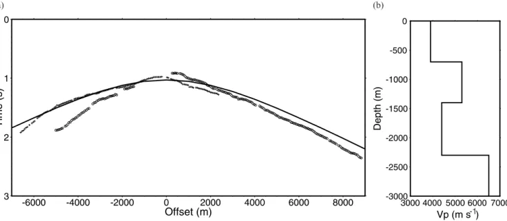
Over 6400 first-arrival times were handpicked on 32 record sec-tions. These sections were selected based on the clarity of first-arrivals and the receiver locations along the profile, in order to en-sure homogeneous data coverage (Fig. 2). The maximum offset for detecting first arrivals ranges from 8000 m to 13 000 m. Very clear impulsive first arrivals, observed up to about 4000 m offset, were assigned a t1–t2 window of 0.01 s, which is equal to a quarter of the dominant period. At larger offsets, the estimated width of t1–t2 window ranges from 0.02 to 0.08 s depending on the offset (Fig. 3c). Concerning the reflection phases, the most noticeable features are large amplitude wide-angle reflections, which display an excel-lent phase coherence and lateral continuity at offsets larger than 5000 m on many CRG record sections (‘event A’ in Figs 3a and b). In order to correlate the observed reflections to geological disconti-nuities known from well data, we computed the expected reflection travel times in a 1D velocity model inferred from VSP data (Fig. 4). The theoretical traveltime curves suggest that these large ampli-tude events may be interpreted as post-critical reflections from a first-order crustal discontinuity drilled at a depth of about 2300 m (1250 mbsl), the latter representing a target for the seismic explo-ration in the survey area.
However, due to the presence of many reflection events on each record section in the wide-angle offset range, the consistent identi-fication of ‘event A’ is problematic especially in regions with low signal-to-noise ratio. In order to ensure a correct phase identifica-tion, we took advantage of data redundancy and used reciprocity relationships between CRG record sections (Fig. 3).
On the other hand, within the near-vertical offset range, the signal-to-noise ratio is low and no clear and continuous near-vertical inci-dence events appear (Fig. 3). In order to identify ‘event A’ at small offsets, we also analysed data arranged in Common Mid-Point gath-ers (CMP), this data arrangement being more suitable to study near
5km
0
2.5
1
2
3
4
5
6
7
8
9
N
Figure 1. Tectonic setting of the wide-angle seismic experiment. (1) Plio-Pleistocene clastic deposits, (2) Cenozoic clayey sediments; (3) Mesozoic basinal rocks; (4) normal faults; (5) thrusts; (6) synclines; (7) anticlines; (8) seismic profile; (9) well for oil exploration.
Figure 2. Topography along the seismic profile and location of the receivers used for the transmission tomography (stars).
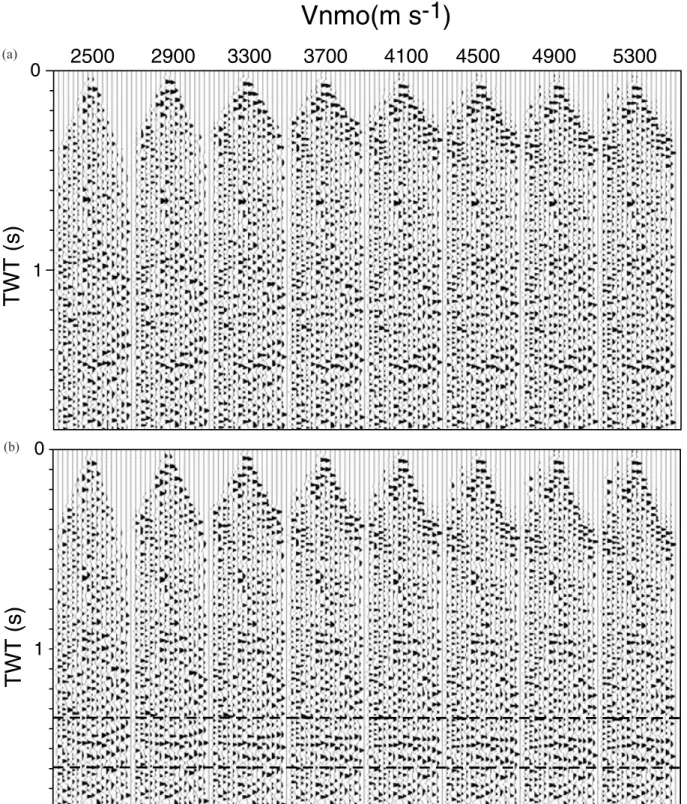
vertical-reflections. The application of tomo-statics (tomography plus static corrections; Zhu et al. 1992) and of the CVS (Constant Velocity Stack) method favoured identification and picking of ‘event A’ at offset smaller than 4000 m on several CMP gathers (Fig. 5).
These reflection traveltime picks were then used as constraints (in addition to reciprocity relationships) for the identification of ‘event A’ on CRG sections. It is interesting to note that the normal move-out velocities estimated for ‘event A’ range from 3000 to 4600 m s−1,
Figure 3. Common receiver gathers from the receiver R126 (a) and R273 (b) (see the location on Fig. 2). First-arrival (time t1) and reflection traveltime curves of the ‘event A’ are superimposed on data. Two examples of reciprocity points amongst the two receivers are also showed (large circles). Data from the receiver R126 display at about−2000 m offset evident times shifts produced by both the rough topography (see Fig. 2) and near-surface low-velocity layers. Data processing includes an AGC window of 0.5 s and a zero-phase trapezoid bandpass filter (5-10-40-50 Hz). (c) Example of first-arrival traveltimes picked (time t1 continuous line, time t2 dashed line) on traces from receiver R126.
(a) (b)
-1
Figure 4. (a) Reflection traveltimes of ‘event A’ picked on the CRG sections for the receivers R126 (circles) and R273 (crosses) are superimposed on the theoretical traveltime curve (continuous line) of the P-to-P reflected phase from the interface at 2300 m of depth. (b) Velocity-depth curve of the 1D model used to compute theoretical reflection traveltimes. This model is based on VSP data.
thus suggesting the presence of significant lateral velocity variations above the target interface.
Finally, over 1600 reflection traveltimes were handpicked on 17 CRG sections with uncertainties ranging from 0.02 s to 0.11 s. Unlike the first arrivals, uncertainties in the reflection traveltime readings decrease with the offset due to the clarity of post-critical reflections.
3 M E T H O D O L O G Y
The inversion scheme tested in this paper is a two-step procedure. The first step is the estimation of a velocity model by first-arrival traveltime tomography. Then, this model is used as the background velocity model to perform an interface inversion.
The extreme complexity of the investigated medium on one hand, and the acquisition lay-out deployed only on the surface, on the other hand, generate a strongly non-linear relation between arrival times and model parameters. Furthermore, we decided not to incorporate any a priori information on the medium in our inversion procedure. For these reasons, both inversion methods use a non-linear optimiza-tion scheme to explore the model parameters space. In the following sections we briefly summarize the two inversion methods.
3.1 Non-linear first-arrival traveltime tomography
Estimation of a reliable background velocity model is a basic re-quirement for the proper inversion of reflection data. Traditionally, velocity models are determined by applying standard velocity anal-ysis (based on the 1D velocity approximation) to near-vertical in-cidence data. Alternatively, we used first-arrival traveltime tomog-raphy, which is a powerful tool to image laterally varying crustal structures when wide-angle refraction data are available (for in-stance, Zhang & McMechan 1994; Zelt & Barton 1998).We used an inversion method which is specially designed to determine strongly heterogeneous velocity models. We shall now review the main fea-tures of this method, which was proposed by Herrero et al. (1999).
A finite-difference Eikonal solver (Podvin & Lecomte 1991) al-lows the fast and accurate estimation of first-arrival traveltimes ac-counting for transmitted, diffracted or head waves in the presence of strongly heterogeneous medium. This is a considerable advantage in our case. Indeed, due to the wide angle acquisition geometry and to severe velocity contrasts, we expect to find at large offsets first arrivals corresponding to head waves. This is why we retained the finite-difference Eikonal solver, in spite of the risk that it might pro-vide first arrival traveltimes corresponding to low amplitude unde-tectable arrivals, owing to its inability to take into account the phase amplitudes.
The velocity model is parametrized by a bi-cubic spline (see for instance Lutter et al. 1990). The inversion strategy is based on a multiscale approach and on a non-linear optimization scheme. A series of inversions is run by progressively refining the velocity grid, the starting model for each inversion being the final model of the previous one. This procedure, which was introduced for velocity estimation by Lutter et al. (1990), allows us first to determine the large-scale components of the velocity model and then to estimate progressively the smaller-scale components.
The choice of a non-linear approach, instead of a linearized to-mographic inversion as done by Lutter et al. (1990), is tied to the strong heterogeneity of the investigated medium. Due to the pres-ence of severe velocity inversions and lateral velocity variations, the definition of a reliable initial velocity model is a challenge, despite of the availability of subsurface information. In such a case, the risk exists that a linearized approach may fail if the used a priori ref-erence velocity model is too far from the actual velocity structure, even using a multiscale strategy (e.g. Bunks et al. 1995). The cost function used in the inversion is a least-squares L2norm, defined as
the sum of the weighted squared differences between observed and computed traveltimes. Data weighting is associated with the inverse t1–t2 time window.
At each inversion run, a search for the model parameters min-imizing the cost function is performed through an hybrid scheme which combines a global random search based on a Monte Carlo technique, and the simplex local optimization technique (Nelder &
0
1
2500
2900
3300
3700
4100
4500
4900
5300
Vnmo(m s
-1
)
0
1
(a) (b)Figure 5. (a) Application of NMO corrections to a representative CMP gather. (b) As in a) but after tomo-statics. Tomo-statics are implemented using the tomographic velocity model (see Fig. 6) and a datum plane placed at the sea level (1100 m below the highest topography). ‘Event A’ (dashed box) is evident after static corrections.
Mead 1965); (a short review of the simplex technique can be found in Jin & Beydoun 2000). Both methods only require the computa-tion of the cost funccomputa-tion and not of its derivatives. We use this hybrid scheme in order to decrease the computational cost, as well as to reduce the chance of trapping in secondary minima of the cost func-tion. Indeed, a straightforward application of a global optimization method based on a Monte Carlo technique would be computationally too expensive, whereas the simplex algorithm could carry the risk of
local convergence due to the high non-linearity of the tomographic problem.
3.2 Non-linear interface inversion
The adopted reflection traveltime inversion method is designed to image rough reflectors embedded in an a priori known, laterally inhomogeneous velocity model. The model parametrization and the
forward traveltime modelling used in the interface inversion are based on a method proposed by Amand & Virieux (1995).
The reflection traveltime for a source–receiver pair and for a given interface is computed by a three-step procedure. Initially, first arrival traveltimes from each source and receiver to the nodes of a regular grid are computed by the fast time estimator of Podvin & Lecomte (1991). These traveltimes are computed in the background velocity model and stored in time tables. Then, based on the time tables, the one-way traveltimes for a source–receiver pair to each point of a given interface are computed performing an interpolation among the nearest four grid nodes. Finally, according to Fermat’s principle, the reflection point for a source–receiver pair and for a given interface will be the one providing the minimum total traveltime.
A bi-cubic spline, interface model parametrization is used (Virieux & Farra 1991). The interface nodes are equally spaced at fixed horizontal locations and can move vertically with continu-ity within a given depth range. The cost function is a least squares
L2 norm, defined as the sum of the weighted squared differences
between observed and theoretical traveltimes. Similarly to the first-arrival inversion method, the inversion strategy follows a multiscale approach and employs a non-linear optimization technique (a mod-ified version of the simplex technique proposed by Nelder & Mead 1965). A series of inversions is run by progressively increasing the number of interface position nodes, as done by Lutter & Nowack (1990). At each inversion run, we generate the vertices (starting in-terface models) of the initial simplex by randomly perturbing in a given depth range the minimum cost interface model obtained in the previous run. The smaller is the spacing of the interface nodes, the smaller is the used depth range.
4 2 D B A C KG R O U N D V E L O C I T Y M O D E L
Over 6400 first arrivals were used to determine a background veloc-ity model by the traveltime tomography. The application to highly redundant data makes the inversion process very stable and robust and allows for a reliable and an accurate model building.
In order to avoid border effects, the model was extended 1000 m southwestward of the first source and 800 m northeastward of the last one. No a priori information about the model was used. Trav-eltimes were computed by a regular grid with a 50× 50 m spacing. A succession of four inversions was run by inverting 12-, 32-, 96-and 128-node models. Each inversion run was halted as soon as the cost function stopped decreasing during the last 5000 iterations. In all the performed runs, a smaller minimum of the cost function was reached by increasing the number of velocity nodes. Running the 128-node inversion, we obtained a final velocity model that is characterized by a RMS traveltime residual of 0.04 s (close to the average uncertainty in time reading).
The final 128-node model (16 horizontal nodes and 8 vertical nodes corresponding to a node spacing of 1000× 537 m) (Fig. 6a) has small first-arrival time residuals confined in the±0.03 s time range (Fig. 6d). Larger residuals, up to 0.07 s, are occasionally observed at offsets smaller than 500 m; they are caused by near-surface small-scale features which are not well modelled due to the poor spatial resolution.
The model resolution was studied by an a posteriori checkerboard test (Hearn & Ni 1994). The perturbation added to the final tomo-graphic image in order to obtain the checkerboard model consists of a 16×8 cells pattern with a maximum perturbation of ±50 m s−1 (Fig. 6b). Such a small amount of perturbation is chosen in order to
avoid changing the wave path in the medium. The inversion proce-dure is then applied to synthetic first-arrival times computed for the checkerboard model. Fig. 6(c) displays the recovered perturbation pattern, which is obtained by subtracting, point by point, the refer-ence and the retrieved checkerboard models. This image gives direct information on how data and the method used are spatially sensi-tive to the shape and amplitude of small velocity perturbations in the final tomographic image. A quantitative assessment of the spa-tial resolution is obtained by measuring the local cross-correlation between the know and recovered checkerboard model around each node. This approach is similar to the one proposed by Zelt (1998), which is based on a semblance function. The best resolved region (with a correlation larger than 0.5) extends from the surface to about 1400–1800 mbsl. between 5000–12 000 m. Resolution progres-sively deteriorates with depth and is low on both sides of the model, where the perturbation pattern is not retrieved at depths larger than 500–1000 mbsl.
The final model displays significant lateral and vertical velocity variations. A broad anticlinal isovelocity feature is evident between 8500 and 12 000 m from the surface down to about 500 mbsl. Inside the anticlinal structure, a high velocity (5000–5300 m s−1) region is broken off by a vertical velocity inversion placed at about 200 mbsl, thus grading into a low velocity (4600–5000 m s−1) region. On the eastern flank of the anticlinal feature, an abrupt deepen-ing of the 3750–4500 m s−1 isovelocity lines occurs. Conversely, to the west, the anticlinal structure blends into a near surface syn-clinal feature with velocities ranging from 2000 to 3500 m s−1. A sharp velocity increase from 5000–5500 m s−1 up to 6000 m s−1 is evident between 6000 and 11 000 m at depths larger than 1500–2000 mbsl.
5 A P P L I C AT I O N O F T H E I N T E R FA C E I N V E R S I O N T O ‘ E V E N T A’
Over 1600 near-vertical/wide-angle reflection traveltimes of ‘event A’ were used to the test the interface inversion method previously de-scribed. The one-way traveltime tables were computed by a squared grid with a 50 m spacing and the 128-node velocity model was used as background reference medium. Reflection traveltimes were weighted by a factor that inversely depends on the uncertainty in the arrival time reading.
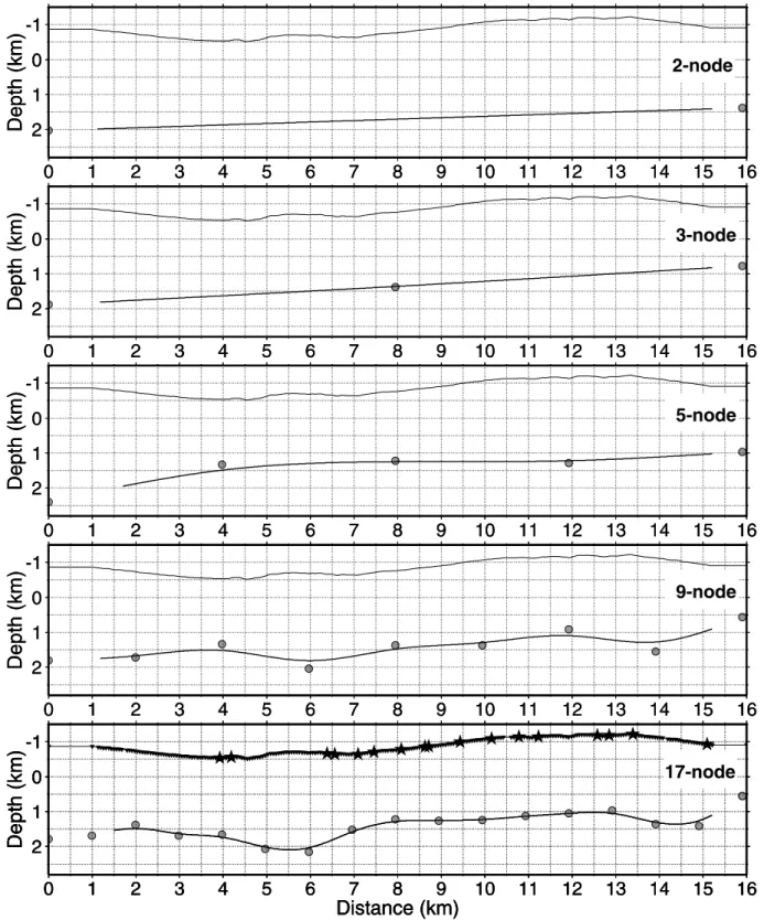
A succession of five interface models parametrized by 2, 3, 5, 9 and 17 nodes were progressively inverted (Fig. 7). Moving from a small to a larger number of interface position nodes we always observed a decrease of the final value of the cost function. The inversion procedure stopped after the fifth run, since the RMS for the minimum cost 17-node model (0.07 s) was close to the average error on arrival time readings (0.06 s).
Fig. 8 shows the arrival time residuals vs positions of the predicted reflection points along the 17-node interface. In the 8000–12 500 m distance range, reflection points are very dense and associated with small time-residuals (±0.1 s) centred at zero. On the other hand, on the lateral model borders, the density of the reflection points strongly decreases, the time residuals are scattered over a much wider range (−0.11/+0.28 s on the western side and −0.15/+0.23 on the eastern side) and are clearly not centred at zero.
The uncertainty in depth of the interface nodes was estimated by locally exploring the variation of the cost function around the minimum cost model. The procedure consists of varying the verti-cal position of a single node within a depth range (±500 m) with a small sampling rate (10 m), fixing the other nodes at the depth
(a)
(b)
(c)
(d)
Figure 6. (a) The final velocity model determined by first-arrival traveltime tomography. This model is parametrized by 128 nodes (black solid circles). The best resolved region of the model extends from the topographic surface down to the black dashed line. The well location is showed. (b) Perturbation pattern used to perform the checkerboard resolution test. The perturbation consists of a 16×8 cell pattern with a maximum perturbation of ±50 m s−1centred on each node. (c) Retrieved perturbation pattern. (d) First-arrival time residuals for two representative CRG sections. The time residuals are computed for both times t1 and times t2. The receiver positions are depicted by triangles.
3-node
17-node
9-node
5-node
2-node
Figure 7. Minimum cost interface models obtained by performing a succession of five inversion runs with an increasing number of interface nodes (gray solid circles). The interface inversion technique is applied to over 1600 reflection traveltime of ‘event A’ picked for the receiver (stars) and source (triangles) displayed in the lower panel. The background reference medium used to compute reflection traveltimes is showed in Fig. 6(a).
values they have in the minimum cost model. The variation of the cost function is computed for each parameter and converted in prob-ability density function using the mean data error as normalization. The uncertainty in depth of the nodes (Fig. 9) is clearly correlated with the time residuals (Fig. 8a), the density of the reflection points (Fig. 8b) and the background model resolution. Indeed, the best
re-solved part of the interface extends from 8000 to 12 000 m, whereas large uncertainties in the shape and location affect both sides of the interface model.
It must be noted that errors on the position and shape of the inter-face also depend on the variability of the incidence angle range at the reflection points along the interface. Figs 10(a)–(c) show three
Ele
v.a.s
.l.
(m)
(a) (b)Figure 8. Reflection time residuals (a) are plotted as a function of the reflection point positions along the 17-node interface (b).
Ele
v.a.s
.l.
(m)
Figure 9. Uncertainty in depth of the interface nodes estimated by locally exploring the variation of the cost function around the final interface model. The variation of the cost function for each parameter (interface node) is computed by varying its depth in the±500 m range and fixing the other parameters at the depth values they take in the minimum cost model. The cost function is converted in probability density function using the mean data error as normalization. The error bars correspond to the 90 per cent of probability. The lower boundary (dotted line) of the best resolved region of the background velocity model is also showed.
examples of ray diagrams, which were built by a posteriori back-ray tracing procedure described by Podvin & Lecomte (1991). Ray cov-erage includes both wide-angle and near-vertical reflections in the central part of the interface (8000–12 000 m) (Figs 10b and c). On the contrary, on the model sides, the interface is sampled exclusively by near-vertical reflections associated with large time residuals (Figs 10a and c). Therefore, the massive use of wide-angle data, in addition to near-vertical data, leads to better inversion results. This is due to the increased data coverage and to the accuracy of the reflection traveltime picks at large offsets, because of the clarity of the post-critical reflections. Moreover, as indicated by synthetic tests (Improta et al. 2000), the modelling of wide-angle data allows
to better constrain the shape of the interface since changes in dip of the predicted interface modify more wide-angle reflection travel paths than near-vertical reflections.
It is interesting to note that ray-paths are strongly distorted by lateral velocity variations. As a consequence, reflection traveltimes picked at progressively increasing offsets can show very different travel paths and may be associated with predicted reflection points placed at a large distance (Fig. 10b). This feature may explain sud-den changes in traveltime, amplitude and waveform, which in some cases affect ‘event A’ within the wide-angle offset range (see for example the post-critical reflections at offsets larger than 7200 m in Fig. 3a).
Ele v.a.s .l.(m) Ele v.a.s .l.(m) Ele v.a.s .l.(m) (a) (b) (c)
Figure 10. (lower panel) Back ray-tracing of the modelled reflection phase (‘event A’) in the background velocity model and (upper panel) reflection time residuals for three receivers (stars) located in the left (a), central (b) and right part (c) of the seismic line.
6 T I M E A N D O F F S E T M O V E - O U T O F ‘ E V E N T A’
The interface inversion method allows us to estimate the position of the reflection point along the minimum-cost interface model for each modelled traveltime. Therefore, the modelled data can be gathered in new panels as a function of the predicted reflection point positions and corrected for the computed reflection traveltime. This procedure is similar to a move-out scheme but using a laterally inhomogeneous background medium and a rough interface. In case of no error on location and shape of the interface, the modelled reflection events should align at 0 s and should show a lateral coherence on the moved-out panels. Therefore, reliability of the determined interface can be verified by measuring the alignment of reflection events on the moved-out gathers by an horizontal stacking of the traces.
Figs 11(a) and (b) show two examples of time and space moved-out gathers. These panels gather traces associated with reflection points for distances comprised in the 8500–12 600 m range (where the interface is well resolved) (Fig. 11c). On the panel displayed in Fig. 11(a), which gathers data from the receivers located on the right side of the model, the alignment and coherence of ‘event A’ are excellent for reflection point distances lower than 11 000 m. At larger distances, the phase alignment is less clear, the reflection points being associated with weak near-vertical reflections picked in regions with low signal-to-noise ratio (see for instance the near-vertical data showed in Fig. 3b). The phase alignment and coherence are proved by the horizontal stacking of the traces, which clearly shows a coherent signal at 0 s.
On the panel gathering the traces for receivers located on the left side of the model (Fig. 11b), the alignment of ‘even A’ is evident for reflection point distances in the 8500–10 000 m range and larger than 10 500 m. The horizontal stacking confirms a phase alignment at about 0 s. In addition, it shows a further coherent signal at about −0.3 s, which results from the stacking of large amplitude first-arrivals for reflection point distances lower than 9500 m. This is not surprising, since first-arrival pulses and ‘event A’ often display similar apparent velocities on CRG sections in the intermediate (3000–6000 m) offset range (Fig. 3a).
It is interesting to note that both near-vertical (NVR) and wide-angle reflections (WR) associated with nearby reflection points align on the panels displayed in Figs 11(a) and (b). This is an a
poste-riori validation of the velocity model reliability. Indeed, given the
different travel path of the near-vertical and wide-angle reflections, only an accurate velocity model would produce an alignment of the reflection events, whatever offset data are used.
7 C O M PA R I S O N W I T H V S P D AT A
The obtained velocity and interface models were compared to VSP data acquired on the seismic line (Fig. 1). As the VSP sampling (20 m) was largely smaller than the vertical node spacing of the velocity model (537 m), the VSP profile was low-pass filtered
(λ < 1 km) in order to cut-off the small-scale components which can
not be solved by the tomographic inversion (Fig. 12). The velocity-depth curve inferred by the tomographic model matches well the fil-tered VSP profile from the surface to about 2400 mbgl (1300 mbsl). At larger depth, where resolution of the background model is low (Fig. 6c), the agreement between the two velocity-depth curves pro-gressively decreases.
VSP data fully confirm the interface inversion results. Indeed, the depth difference between the retrieved interface and the sharp
first-order velocity contrast associated with the target discontinuity (drilled at about 1250 mbsl) is about 40 m.
Surface geology and well information allow to associate features of the velocity model with geological units. The broad anticlinal isovelocity feature imaged from 8500 to 12 000 m (Fig. 6a) is in agreement with the antiform mapped in Fig. 1. The well, which ex-plored this structure, drilled a system of thrusts involving Mesozoic basinal rocks: two thrust sheets, mainly composed of high veloc-ity (5200–5500 m s−1) cherty limestones, overlay tectonically at 300 mbsl a succession of shales and cherts characterized by lower seismic velocities (Fig. 12). Therefore, on the basis of well data, the high velocity (5000–5300 m s−1) region located inside the anticli-nal feature and the underlying low velocity (4600–5000 m s−1) layer may be associated with the limestone thrusts and with shaley/cherty strata, respectively. Moreover, the abrupt deepening of the isove-locity lines on the eastern flank of the antiform, is indicative of the thrust structure and correlates with the surface outcropping of a thrust ramp eastward of the seismic line. To the west, the near-surface synclinal isovelocity feature is in agreement with a synform filled by Cenozoic clays and Pliocene sands. In addition, the deep-ening of the 2000–3000 m s−1 isovelocity lines at about 6000 m matches well the NW–SE trending axis of the syncline.
The interface determined by reflection traveltimes inversion may be associated with the top of a cherty limestone succession. This interpretation, that is locally proved by well information, may be extended to the 6000–11000 m distance range, where the retrieved reflector follows the top of the high velocity (5500–6000 m s−1) region imaged by tomography (Fig. 6a) and the velocity model res-olution is high (Fig. 6c).
8 D I S C U S S I O N A N D C O N C L U S I O N S
In this paper, we tested a two-step procedure for the separate in-version of first arrival and reflection traveltimes with a multi-fold wide-angle data set. Transmission tomography is used to determine a smooth velocity model, which is then employed as the background reference medium for a subsequent interface inversion. This proce-dure is specially designed to image rough reflectors embedded in strongly inhomogeneous media by modelling dense data (acquired with a wide-angle geometries) and is able to operate with a rough topography, unevenly spaced data and in presence of severe lateral and vertical velocity variations.
Both inversion methods employ a fast technique for the forward problem solution based on the finite-difference Eikonal solver of Podvin & Lecomte (1991). The speed in the forward problem solu-tion favours the use of an inversion strategy to perform a massive exploration of the model parameters (velocity or interface position nodes). The strategy for model space exploration, which is similar for both inversion techniques, is based on a multiscale approach and on a non-linear optimization scheme. The choice of a non-linear ap-proach is tied to the high degree of non-linearity between arrival traveltimes and model parameters, due both to the strong hetero-geneity of the investigated medium and to the acquisition lay-out, which is deployed only on the surface. The incorporation of a non-linear optimization scheme into a multiscale approach makes the model parameters estimation more stable and robust, reducing the risk of local convergence.
The testing with the wide-angle data set collected in the South-ern Apennines (Italy) reveals the advantages of the application of this inversion procedure in an on-land thrust belt environment, where conventional near-vertical reflection seismic failed to provide
8500
10000
9500
9000
10500
12500
12000
1
1500
1
1000
SF
A
Distanceoftheassociatedreflectionpoint(m)
NVR
WRWR
LF
A
8500
10000
9500
9000
10500
12500
12000
1
1500
1
1000
SF
A
SF
A
LF
A
NVR
WRWR
(a)
(b)
(c)
Figur e 11. T ime and space mo v ed-out sections g athering data recorded b y the recei v ers located on the right (a) and on the left (b) of the w ell. (c) P osition of the so urces (triangles), of the recei v ers (stars) and of the predicted re fl ection points (circles) along the interf ace (dashed line). The traces are cor rected for the estimated tra v eltimes of the modelled re fl ected phase (‘ ev ent A ’ outlined b y a g ra y band) and plotted as a function of the predicted re fl ection point positions along the retrie v ed interf ace. The horizontal stacking of the traces allo ws to measure the alignment and coherence of the mode lled phase. SF A for small-of fset fi rst-ar ri v al, LF A for lar ge-of fset fi rst-ar ri v al, NVR for near -v er tical re fl ection, WR for wide-angle re fl ection.Figure 12. Comparison of the inversion results with well information. (1) shales (Lower Cretaceous); (2) cherts (Jurassic-Upper Triassic); (3) cherty limestones (Upper Triassic); (4) sandstones (Middle-Lower Triassic); (5) main thrust planes; (6) velocity-depth profile determined by VSP data; (7) low-pass (λ > 1000 m) filtered VSP velocity-depth profile; (8) velocity-depth curve inferred by the 2D tomographic model.
good-quality images because of the complexity of the velocity field and of a rough topography (Dell’Aversana 2001).
The use of dense large offset refraction data, which contain rel-evant information on the velocity distribution in depth, along with the use of a robust non-linear inversion technique for velocity opti-mization, enabled us to produce a detailed and reliable tomographic model down to a maximum depth of 2500–3000 m from the surface (Figs 6a and c). Despite the extreme complexity of the investigated structure, which also includes severe velocity inversions, this model is consistent with the VSP data (Fig. 12) and clearly outlines anti-clinal and synanti-clinal structures.
The availability of an accurate laterally inhomogeneous velocity model, subsequently enabled us to take advantage of the relevant information carried by post-critical reflections (dominant in ampli-tude in the wide-angle offset range). This was performed by an
inter-face inversion of reflection traveltimes picked in the complete offset range. The inversion results, which are consistent with well informa-tion (Fig. 12), and synthetic tests (Improta et al. 2000), show that the use of redundant wide-angle data in addition to near-vertical reflec-tions allows to reduce the uncertainty in the interface detection. In addition to the increased data coverage, the wide-angle components heavily contribute to the robustness of the inversion for two further reasons: (a) post-critical reflections picks are usually affected by small uncertainties due to the clarity of the events, (b) wide-angle data provide additional constraints on the interface shape, since a change in dip of the predicted interface strongly modifies the travel path and arrival time of wide-angle reflections. These advantages become evident in thrust belt regions, where the collection of high quality data by near-vertical seismic experiments may be a difficult task.
In addition, as the topography is directly included in the interface inversion, no static corrections are required. This is a great advan-tage considering that the theoretical and practical extension of the methods for static computation to thrust belt regions with rugged terrain remains a challenge (Schneider et al. 1995; Bevc 1997; Zhu
et al. 1998). To sum up, our applications demonstrate that the
inver-sion procedure can be efficient for target-orientated studies of the upper crust in complex geological environments, such as in thrust belts.
Of course, the method suffers from some limitations. First, as the accuracy of the background model has a strong influence on the interface inversion results, the target-zone is limited in depth to the best resolved region of the velocity model, whose lower bound-ary critically depends on the maximum offsets for usable refracted energy. In our case, due to the low resolution of the velocity model for depths larger than 2500–3000 mbgl, the potential target-zone is limited to the shallow crust. A possible strategy to overcome this limitation is to enlarge the spread of the acquisition geometry in order to increase the exploration depth of the transmission tomog-raphy. This strategy was successfully used by Dell’Aversana et al. (2001) in a wider-angle survey performed recently in the Southern Apennines. Indeed, a detailed velocity model was produced down to a depth of 5000 mbgl by applying transmission tomography to redundant refracted data collected up to 25 000 m offset.
Another limitation of the procedure is the non-negligible human intervention required to pick reflection traveltimes. In order to avoid this limitation and to improve the time performance of the whole procedure, our future efforts will focus on the use of a different objective function in the interface inversion based on coherence measures. A possible approach could be based on the measure of the alignment of the target events on time and space moved-out panels (see Section 6) by data staking. Besides, this improvement in time performance would facilitate the theoretical and practical extension of the inversion procedure to 3D wide-angle data set.
A C K N O W L E D G M E N T S
We would like to thank Sergio Morandi of Enterprise Oil Italiana for his support and suggestions. The very useful comments and En-glish reviewing of C. Piromallo and S. Nielsen are greatly acknowl-edged. We acknowledge two anonymous reviewers and Prof. Roul Hadoruege. This study has been financially supported by Enterprise Oil Italiana.
R E F E R E N C E S
Amand, P. & Virieux, J., 1995. Non linear inversion of synthetic seismic reflection data by simulated annealing, 65th Ann. Internat. Mtg: Soc. Expl.
Geophy. Expanded Abstracts, 612–615.
Bevc, D., 1997. Flooding the topography: Wave equation datuming of land data with rugged acquisition topography, Geophysics, 62, 1558–1569. Bunks, C., Saleck, F.M., Zaleski, S. & Chavent, G., 1995. Multiscale seismic
waveform inversion, Geophysics, 60, 1457–1473.
Dell’Aversana, P., 2001. Integration of seismic, MT, and gravity data in a thrust belt interpretation, First Break, 19, 335–341.
Dell’Aversana, P., Ceragioli, E., Morandi, S. & Zollo, A., 2000. A
simulta-neous acquisition test of high density “global offset” seismic in complex geologicalal settings, First Break, 18, 87–96.
Dell’Aversana, P., Zucconi, V. & Colombo, D., 2001. Improvement in seismic acquisition by 3D Global offset approach, 71st Ann. Internat. Mtg: Soc.
Expl. Geophy. Expanded Abstracts, 29–32.
Hearn, T.M. & Ni, J.F., 1994. Pn velocities beneath continental collision zones, Geophys. J. Int., 117, 273–283.
Herrero, A., Zollo, A. & Virieux, J., 1999. 2D Non linear first arrival time inversion applied to Mt. Vesuvius active seismic data (TomoVes96), Eur.
Geophys. Soc.,, XXIV, General Assembly, 19–23 April, 1999, The Hague,
The Netherlands.
Improta, L., Zollo, A., Frattini, M.R., Virieux, J., Herrero, A. & Dell’Aversana, P., 2000. Mapping interfaces in an overthrust re-gion by non-linear traveltime inversion of reflection data, Am.
geophys. Un.,Fall Meeting, 15–19 December 2000, San Francisco,
USA.
Jin, S. & Beydoun, W., 2000. 2D multiscale non-linear velocity inversion,
Geophys. Prospect., 48, 163–180.
Jin, S. & Madariaga, R., 1994. Nonlinear velocity inversion by a two step Monte Carlo method, Geophysics, 59, 577–590.
Kodaira, S., Takahashi, N., Nakanishi, A., Miura, S. & Kaneda, Y., 2000. Subducted seamount imaged in the rupture zone of the 1946 Nankaido earthquake, Science, 289, 104–106.
Lynn, W.S. & Claerbout, J.F., 1982. Velocity estimation in laterally varying media, Geophysics, 47, 884–897.
Lutter, W.J. & Nowack, R.L., 1990. Inversion of crustal structure using re-flections from the PASSCAL Ouachita Experiment, J. geophys. Res., 95, 4633–4646.
Lutter, W.J., Nowack, R.L. & Braile, L.W., 1990. Seismic imaging of the upper crustal structure using travel times from the PASSCAL Ouachita Experiment, J. geophys. Res., 95, 4621–4631.
Mazzotti, A.P., Stucchi, E., Fradelizio, G.L., Zanzi, L. & Scandone, P., 2000. Seismic exploration in complex terrains: a processing experience in the Southern Apennines, Geophysics, 65, 1402–1417.
Nelder, J.A. & Mead, R., 1965. A simplex method for function minimization,
Comput J., 7, 308–313.
Podvin, P. & Lecomte, I., 1991. Finite difference computation of traveltimes in very contrasted velocity model: A massively parallel approach and its associated tools, Geophys. J. Int., 105, 271–284.
Samson, C., Barton, P.J. & Karwatowski, J., 1995. Imaging beneath an opaque basaltic layer using densely sampled wide-angle OBS, Geophys.
Prospect., 43, 509–527.
Schneider, W.A., Phillip L.D. & Paal, E.F., 1995. Wave-equation velocity replacement of the low velocity layer for overthrust-belt data, Geophysics, 60, 573–579.
Virieux, J. & Farra, V., 1991. Ray tracing in 3D complex isotropic media: An analysis of the problem, Geophysics, 56, 2057–2069.
Zelt, C.A., 1998. Lateral velocity resolution from three-dimensional seismic refraction data, Geophys. J. Int.,135, 1101–1112.
Zelt, C.A. & Barton, P.J., 1998. Three-dimensional seismic refraction to-mography: a comparison of two methods applied to data from the Faeroe Basin, J. geophys. Res., 103, 7187–7210.
Zelt, B.C., Talwani, M. & Zelt, C.A., 1998. Prestack depth migration of dense wide-angle seismic data, Tectonophysics, 286, 193–208. Zhang, J. & McMechan, G.A., 1994. 3D transmission tomography using wide
aperture data for velocity estimation for irregular salt bodies, Geophysics, 59, 1620–1630.
Zhu, X., Angstmon, B.G. & Sixta, D.P., 1998. Overthrust imaging with tomo-datuming: A case study, Geophysics, 63, 25–38.
Zhu, X., Sixta, D.P. & Angstman, B.G., 1992. Tomo-statics: Turning-ray tomography+ static corrections, The Leading Edge, 11, 15–23.