Publisher’s version / Version de l'éditeur:
Vous avez des questions? Nous pouvons vous aider. Pour communiquer directement avec un auteur, consultez la
première page de la revue dans laquelle son article a été publié afin de trouver ses coordonnées. Si vous n’arrivez pas à les repérer, communiquez avec nous à PublicationsArchive-ArchivesPublications@nrc-cnrc.gc.ca.
Questions? Contact the NRC Publications Archive team at
PublicationsArchive-ArchivesPublications@nrc-cnrc.gc.ca. If you wish to email the authors directly, please see the first page of the publication for their contact information.
https://publications-cnrc.canada.ca/fra/droits
L’accès à ce site Web et l’utilisation de son contenu sont assujettis aux conditions présentées dans le site LISEZ CES CONDITIONS ATTENTIVEMENT AVANT D’UTILISER CE SITE WEB.
Probabilistic Methodologies in Water and Wastewater Engineering (in Honour of Prof. Barry Adams, University of Toronto): 23 September 2011, Toronto, Canada [Proceedings], pp. 1-9, 2011-09-23
READ THESE TERMS AND CONDITIONS CAREFULLY BEFORE USING THIS WEBSITE.
https://nrc-publications.canada.ca/eng/copyright
NRC Publications Archive Record / Notice des Archives des publications du CNRC :
https://nrc-publications.canada.ca/eng/view/object/?id=91aba2d1-f81c-493a-8d64-e37ab2568304 https://publications-cnrc.canada.ca/fra/voir/objet/?id=91aba2d1-f81c-493a-8d64-e37ab2568304
NRC Publications Archive
Archives des publications du CNRC
This publication could be one of several versions: author’s original, accepted manuscript or the publisher’s version. / La version de cette publication peut être l’une des suivantes : la version prépublication de l’auteur, la version acceptée du manuscrit ou la version de l’éditeur.
Access and use of this website and the material on it are subject to the Terms and Conditions set forth at Characterization of external corrosion pits in ductile iron pipes
Characterization of external
corrosion pits in ductile iron
pipes
Kleiner, Y.; Rajani, B.B.
NRCC-54557
A version of this document is published in / Une version de ce document se trouve dans: Probabilistic Methodologies in Water and Wastewater Engineering (in Honour of Prof. Barry Adams, University of Toronto) (Toronto, Canada, September 23-24, 2011, pp. 1-9
The material in this document is covered by the provisions of the Copyright Act, by Canadian laws, policies, regulations and international agreements. Such provisions serve to identify the information source and, in specific instances, to prohibit reproduction of materials without written permission. For more information visit http://laws.justice.gc.ca/en/showtdm/cs/C-42
Les renseignements dans ce document sont protégés par la Loi sur le droit d’auteur, par les lois, les politiques et les règlements du Canada et des accords internationaux. Ces dispositions permettent d’identifier la source de l’information et, dans certains cas, d’interdire la copie de documents sans permission écrite. Pour obtenir de plus amples renseignements : http://lois.justice.gc.ca/fr/showtdm/cs/C-42
1
Characterization of external corrosion pits in ductile iron pipes
Yehuda Kleiner and Balvant Rajani
National Research Council of Canada, Institute for Research in Construction 1200 Montreal Road, Ottawa, Ontario K1A 0R6, Canada
Abstract:
Varying lengths of ductile iron (DI) pipes were exhumed by several North American water utilities. The exhumed pipes were cut into short sections, sandblasted and tagged. Pipe sections were scanned for external corrosion using a specially developed laser scanner. Scanned
corrosion data were processed using specially developed software to obtain information on corrosion depth, area and volume along the pipe. A general definition of corrosion pit was proposed and statistical analyses were subsequently performed on these three geometrical attributes of the pit populations.
Keywords: Ductile iron pipe, corrosion pits, corrosion pit geometry, probability distribution
Introduction
Virtually all the models in the literature that endeavor to propose a relationship between soil characteristics and corrosion rate of buried metallic pipes are empirical, and can generally be divided into two classes, namely, practical and empirical/probabilistic. The most widely known practical approach is the 10-point scoring method proposed by AWWA (Appendix A of
ANSI/AWWA C105/A21.5-99), which classifies a soil as corrosive/noncorrosive based on the weighted aggregation of 5 soil properties. The 25-point scoring method of Spickelmire (2002) is similar to the AWWA 10-point method except that other additional factors are included.
Several researchers have used statistical/probabilistic tools to characterize the properties of corrosion pits. Aziz (1956) used extreme value statistics (EVS) to propose the Gumbel distribution for the analysis of corrosion pit-depth maxima. Hay (1984) also found that the Gumbel distribution fitted corrosion pit-depth maxima well in buried cast iron pipes. Sheikh et al. (1989) proposed a truncated exponential distribution as the underlying distribution for pit
2 depth. Laycock et al. (1990) used the generalized extreme value statistics to analyze corrosion pit-depth maxima. Katano et al. (1995) and Katano et al. (2003) found that the log-normal distribution best fitted their pit data; Melchers (2003, 2004a, 2004b), fitted multi-phase power models (as a function of time) to corrosion data. Melchers (2005a,b,c) questioned the use of extreme value distribution such as Gumbel to represent the distribution of corrosion pit-depth maxima and reasoned that corrosion pits form two populations, one of metastable pits (those pits that initiate but stop growing immediately or a short while after initiation) and stable pits (those pits that continue to grow). Several researchers, including Ferguson et al. (1993), Kalantzis (1997), Restrepo et al. (2009), Caleyo et al. (2009), among others, investigated the impact of various soil properties on the corrosion pit properties of buried pipes.
The National Research Council of Canada (NRC), with funding from the Water Research Foundation (WaterRF), undertook a research project to investigate the long term performance of ductile iron (DI) water mains. One of the objectives of this research was to gain a thorough understanding of geometry of external corrosion pits and the factors (e.g., soil properties, appurtenances, service connections, etc.) that influence this geometry. It was hoped that this understanding would lead to the ultimate objective of achieving a better ability to assess the remaining life of ductile iron pipes for a given set of circumstances. Four North American water utilities exhumed each about 91.4 m (300 ft) of DI pipe, which were cut into sections,
sandblasted and tagged. Soil samples were also obtained at discrete locations along the exhumed pipe. A laser scanner that was specially developed at the NRC to scan the pipe for external corrosion using and special software was developed to process the scanning data and obtain information on pit-depth, pit-area and pit-volume. This paper focuses only on the general definition of corrosion pit and the statistical analysis that follows. He full research report can be found at Rajani et al. (2011).
Data collection, cleansing and preparation
Four water utilities exhumed approximately 91.4 m (300 ft) of ductile iron pipe slated for replacement (Table 1), which were cut into sections (approx. 1 meter long), sandblasted and scanned, using a specially developed laser scanner (Figure 1). Using software specially developed for this purpose, a six-step process was used to record the data and remove these
3 undesired effects: (a) read in raw data and apply a raw data filter; (b) rearrange the data into a grid; (c) establish the “correct” pipe surface; (d) apply 2-D grid-level filter; (e) apply 3-D grid-
Table 1. Details of exhumed pipes
City (Water utility) Pipe diameter Depth Length Installation year
Kansas City (Water One) 300 mm (12”) 1.07 m (3.5’) 91.4 m (300’) 1989 St. Louis (American Water) 300 mm (12”) 1.22 m (4’) 42.7 m (140’) 1970 Louisville (Louisville Water Co.) 200 mm (8”) 1.07 m (3.5’) 91.4 m (300’) 1972 Calgary (Calgary Water Dept.) 250 mm (10”) 3.05 m (10’) 91.4 m (300’) 1969
Figure 1. Pipe scanner (left: pipe mounted ready for scanning; right: laser point range finder mounted on track).
level filter; and (g) remove unusable data for statistical analysis. Details on the various filters applied to the data can be found in Rajani et al. (2011). Statistical analyses were conducted on geometrical properties of corrosion pits including pit-depth maxima, pit-area and pit-volume that were generated from the cleansed scanned data. Two different approaches were investigated as to the definition of the corrosion pit populations to which statistical analysis should be applied, namely individual pit populations and pipe ring populations. In this paper we focus only on individual pit populations and specifically on pit-depth maxima.
Definition and analysis of individual pit population
Corrosion pits are naturally small upon initiation and some will grow over time while others will become passivated (Aziz, 1957, used the term “stifled” and Melchers, 2005c referred to them as metastable (passivated) and stable pits). If two pits in close proximity continue to grow they will eventually combine (coalesce) to form one larger pit. This larger pit can continue to grow and
Pipe Track
4 may combine with yet more adjacent pits to become an even larger pit. This corrosion pit
morphology presents a challenge as to what constitutes a single pit and its associated geometric properties. We used the notion of threshold depth to define a single pit.
Figure 2 illustrates two adjacent corrosion pits that partially coalesced into one. If “Threshold 1” is taken as a reference then we have one corrosion pit with length X1 and maximum depth = (wall thickness - Y2). If “Threshold 2” is taken as a reference then we have two corrosion pits with lengths X2 and X3 and depths = (wall thickness - Y2) and = (wall thickness - Y3),
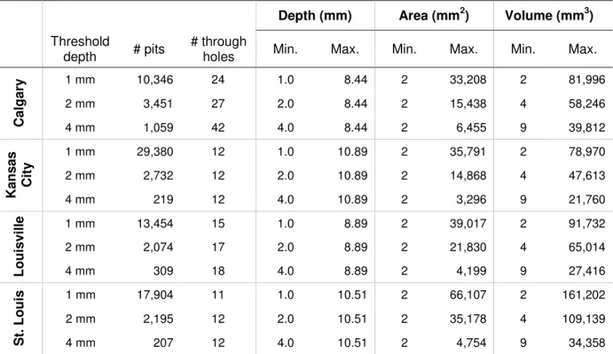
respectively. It is thus clear that a population of pits generated with threshold x is different from a population of pits generated with threshold y, and one population is not a subset of the other. For each of the four cities, three pit populations were generated, with three different threshold depth values as described in Table 2. Note that higher threshold depths result in a lower number of corrosion pits in the population. This is expected because, for example, all pits with depth smaller than 2 mm are not considered when the threshold depth is 2 mm. However, note also that the number of through-holes can increase as the threshold depth increases. This can be explained with the help of Figure 2. Suppose that Y2 and Y3 were zero, i.e., there would be two through-holes in these locations. If the reference threshold depth is “Threshold 2” then there are two pits, each with depth exceeding wall thickness, i.e., two through-holes. However, if the reference threshold depth is “Threshold 1”, then there is only one pit with maximum pit depth exceeding wall thickness. In this case a through-hole is counted only once, even though there could be multiple perforations within the pit.
Figure 2. Corrosion pits and threshold depth
Y3 Y2
5
Table 2 Pit populations generated with various threshold depth values
Depth (mm) Area (mm2) Volume (mm3)
Threshold
depth # pits
# through
holes Min. Max. Min. Max. Min. Max.
C al g ar y 1 mm 10,346 24 1.0 8.44 2 33,208 2 81,996 2 mm 3,451 27 2.0 8.44 2 15,438 4 58,246 4 mm 1,059 42 4.0 8.44 2 6,455 9 39,812 K an sas C it y 1 mm 29,380 12 1.0 10.89 2 35,791 2 78,970 2 mm 2,732 12 2.0 10.89 2 14,868 4 47,613 4 mm 219 12 4.0 10.89 2 3,296 9 21,760 L o u is v ille 1 mm 13,454 15 1.0 8.89 2 39,017 2 91,732 2 mm 2,074 17 2.0 8.89 2 21,830 4 65,014 4 mm 309 18 4.0 8.89 2 4,199 9 27,416 S t. L o u is 1 mm 17,904 11 1.0 10.51 2 66,107 2 161,202 2 mm 2,195 12 2.0 10.51 2 35,178 4 109,139 4 mm 207 12 4.0 10.51 2 4,754 9 34,358
Three different probability distributions as well as their right-truncated variants were examined as candidates to describe the populations of pit-depth maxima, where pipe wall-thickness is the upper bound of the truncated probability distribution. The distributions explored included Weibull (2-parameter), Gumbel (or double-exponential) and the exponential distribution. Probability distribution parameters were discerned using the maximum likelihood method. Pearson’s chi-square test was used to ascertain “goodness of fit” between model and data (in all cases there were sufficient data to warrant chi-square test). Through-holes were excluded in the exploration of probability distributions for pit-depth maxima because they comprise an ever-increasing category of pits with constant depth, which would bias the distribution.
Figure 3 illustrates the fitting of the truncated Weibull distribution to pit maxima derived with 1, 2 and 4 mm pit depth threshold. Chi-square test results are provided as P-values. It can be seen that the truncated Weibull distribution fits the pit-depth maxima data very well. As explained earlier, through-holes were excluded from the analysis of pit-depth maxima.
6
Figure 3. Statistical properties of pit-depth maxima (Calgary) with 1, 2 and 4 mm threshold depth
Truncated Weibull distribution
0 2 4 6 8 10
Pit depth
2 mm pit threshold
Chi square test = 0.021 (P-value = 0.000) 0 2 4 6 8 10 Pit depth 0.00 0.20 0.40 0.60 0.80 1.00 0 2 4 6 8 10 R e la ti v e f re q u e n cy Pit depth 1 mm pit threshold
Chi square test = 0.04 (P-value = 0.000)
4 mm pit threshold
Chi square test = 0.044 (P-value = 0.000) 0% 20% 40% 60% 80% 100% 0 1 2 3 4 5 6 7 8 9 0.001 0.010 0.100 1.000 10.000
Log pit depth
4 mm pit threshold 0% 20% 40% 60% 80% 100% 0 1 2 3 4 5 6 7 8 9 0.001 0.010 0.100 1.000 10.000 0% 20% 40% 60% 80% 100% 0 2 4 6 8 10 0.001 0.010 0.100 1.000 10.000 Theoretical distribution Plotting position of
observed data 1 mm pit threshold
2 mm pit threshold
Probability
Probability
7 The bottom of Figure 3 illustrates the plotting position of the data, linearized using the assumed right-truncated Weibull probability distribution. Note that due to the limitations of log scale, the data were shifted so that pit-depth is taken relative to the respective threshold values. Note also that the straight line was not visually fitted to the data but rather obtained using the distribution parameters that were discerned using the maximum likelihood method. Data that are perfectly distributed according to the assumed model will appear as a straight line on such a linearized plot. Data related to 1 mm threshold appear to be fairly linear for the most part, except at the lower tail of the distribution. This deviation from straight line of the lower tail is all but
eliminated for 2 mm and 4 mm thresholds, which suggests that the deviation could be attributed to the various data filtering methods that were applied during data preparation which may have created some distortion in the very small values of pit depth. Similar results (not shown here) were obtained for the pit data of pipes exhumed in Kansas City, Louisville and St. Louis. The right-truncated Weibull probability distribution was found to fit best the observed frequencies in all four data sets, i.e., Calgary, Kansas City, Louisville and St. Louis, and therefore was deemed to be the most likely underlying probability distribution of pit-depth maxima, regardless of the threshold depth value used. In some cases, the non-truncated and truncated exponential distribution also fit the data fairly well, but never as well as the right-truncated Weibull distribution. This finding is in contrast to observations made by Aziz (1957), and as noted earlier also by Sheikh et al. (1989), who assumed the truncated exponential
distribution and Sheikh et al. (1990), who assumed the normal distribution of the square root of pit depth at the early stage of corrosion and lognormal in the more advanced stages of corrosion.
Concluding comments
The right-truncated Weibull probability distribution was found to fit best the observed frequencies in all four data sets, i.e., Calgary, Kansas City, Louisville and St. Louis, and therefore was deemed to be the most likely underlying probability distribution of pit-depth maxima, regardless of the threshold depth value to used. In some cases, the non-truncated and truncated exponential distribution also fit the data fairly well, but never as well as the right-truncated Weibull distribution. This finding differs from observations made by Aziz (1957), who assumed exponential distribution at an early stage of corrosion and a bi-modal distribution at a later stage as well as from observations by Sheikh et al. (1989), who assumed the truncated
8 exponential distribution and Sheikh et al. (1990), who assumed the normal distribution of the square root of pit depth at the early stage of corrosion and lognormal in the more advanced stages of corrosion.
This investigation of pit populations was conducted to expand on existing knowledge and to compare findings with those of other researchers rather than for any practical purpose. It is much more practical to create sampling schemes and inference methods based on ring population rather than pit population. Practical sampling scheme would typically involve examination of a number of small pipe samples that represents the entire pipe. As the area of a single pit can vary significantly, sample sizes would have to be quite large to contain entire large pits. Furthermore, when a pipe is virtually divided into rings, the location of each ring can be easily related to the location of a soil sample. Moreover, ring-based analysis lends itself better to develop inference techniques that are based on return period computations (Rajani et al., 2011) because a ring is always geometrically well defined.
Acknowledgement
This research project was co-sponsored by the Water Research Foundation (WaterRF), the National Research Council of Canada (NRC) and water utilities from the United States, Canada and Australia.
References
ANSI/AWWA C105/A21.5-99. (1999). “American National Standard for polyethylene encasement for ductile iron pipe systems”. American Water Works Association, Denver, CO. Aziz, P.M. (1956). “Application of the statistical theory of extreme values to the analysis of maximum pit depth data for aluminum”. Corrosion 12, pp. 495t-506t.
Caleyo, F., Velázquez, J.C., Valor, A. and Hallen, J.M. (2009). “Probability distribution of pitting corrosion depth and rate in underground pipelines: A Monte Carlo study”. Corrosion Science, 51, pp. 1925–1934.
Hay, L. S. (1984). “The influence of soil properties on the performance of underground pipelines”. M.Sc.(Agriculture) thesis, Dept. Soil Science, University of Sydney, Sydney, Australia.
9 Katano, Y., Miyata, K., Shimizu, H. and Isogai, T. (1995). “Examination of statistical models for pitting on underground pipes and data analysis”. Proceedings of the International Symposium on plant aging and life prediction of corrodible structures, May 15-18, Sapporo, Japan.
Katano, Y., Miyata, K., Shimizu, H. and Isogai, T. (2003). “Predictive model for pit growth on underground pipes”. Corrosion, 59(2), pp. 155-161.
Laycock, P.J., Cottis, R.A. and Scarf, P.A. (1990). “Extrapolation of extreme pit depths in space and time”. Journal of the Electrochemical Society, 137(1), pp. 64-69.
Melchers, R.E. (2003). “Modeling of marine immersion corrosion for mild and low alloy steels-Part 1: phenomenological model”. Corrosion (NACE), 59(4), pp. 319–334.
Melchers, R.E. (2004a). “Pitting corrosion of mild steel in marine immersion environment – Part 1: maximum pit depth”, Corrosion (NACE), 60(9), pp. 824-836.
Melchers, R.E. (2004b). “Pitting corrosion of mild steel in marine immersion environment - Part 2: variability of maximum pit depth”. Corrosion (NACE), 60(10), pp. 937–944.
Melchers, R.E. (2005a). “Statistical characterization of pitting corrosion – 1: Data analysis”. Corrosion (NACE), 61(7), pp. 655-664.
Melchers, RE (2005b) “Statistical characterization of pitting corrosion – 2: Probabilistic modelling for maximum pit depth”. Corrosion (NACE), 61(8), pp. 766-777.
Melchers, RE (2005c). “Representation of uncertainty in maximum depth of marine corrosion pits”. Structural Safety, 27, pp. 322-334.
Rajani, B., Kleiner, Y., and Krys, D. (2011) “Long-term performance of ductile iron pipe”, Research report #3036, Water Research Foundation, Denver, CO.
Restrepo, A., Delgado, J. and Echeverría, F. (2009). “Evaluation of current condition and lifespan of drinking water pipelines”. Journal of Failure Analysis and Prevention. 9,pp. 541–548.
Sheikh, A.K., Boah, J.K. and Jounas, M. (1989). “Truncated extreme value model fro pipeline reliability”. Reliability Engineering and System safety, 25(1), pp. 1-14.
Sheikh, A.K., Boah, J.K. and Hansen, D.A. (1990). “Statistical modelling of pitting corrosion and pipeline reliability”. Corrosion-NACE, 46(3), pp. 190–197.
Spickelmire, B. (2002). "Corrosion consideration for ductile iron pipe". Materials Performance, 41, 16-23.