Data Analysis for a Model Podded Propulsor in Ice (Pusher Mode)

Publisher’s version / Version de l'éditeur:

Vous avez des questions? Nous pouvons vous aider. Pour communiquer directement avec un auteur, consultez la première page de la revue dans laquelle son article a été publié afin de trouver ses coordonnées. Si vous n’arrivez pas à les repérer, communiquez avec nous à PublicationsArchive-ArchivesPublications@nrc-cnrc.gc.ca.

Questions? Contact the NRC Publications Archive team at

PublicationsArchive-ArchivesPublications@nrc-cnrc.gc.ca. If you wish to email the authors directly, please see the first page of the publication for their contact information.

https://publications-cnrc.canada.ca/fra/droits

L’accès à ce site Web et l’utilisation de son contenu sont assujettis aux conditions présentées dans le site

LISEZ CES CONDITIONS ATTENTIVEMENT AVANT D’UTILISER CE SITE WEB. Student Report; no. SR-2009-05, 2009-01-01

READ THESE TERMS AND CONDITIONS CAREFULLY BEFORE USING THIS WEBSITE.

https://nrc-publications.canada.ca/eng/copyright

NRC Publications Archive Record / Notice des Archives des publications du CNRC :

https://nrc-publications.canada.ca/eng/view/object/?id=9424bd78-6f0e-47d5-8898-f879709ebe08 https://publications-cnrc.canada.ca/fra/voir/objet/?id=9424bd78-6f0e-47d5-8898-f879709ebe08

Archives des publications du CNRC

For the publisher’s version, please access the DOI link below./ Pour consulter la version de l’éditeur, utilisez le lien DOI ci-dessous.

https://doi.org/10.4224/18227306

Access and use of this website and the material on it are subject to the Terms and Conditions set forth at Data Analysis for a Model Podded Propulsor in Ice (Pusher Mode)

Ocean Technology technologies oc ´eaniques

SR-2009-05

Student Report

Data Analysis for a Model Podded Propulsor in Ice

(Pusher Mode).

REPORT NUMBER

SR-2009-05

NRC REPORT NUMBER DATE

April 2009

REPORT SECURITY CLASSIFICATION DISTRIBUTION

TITLE

Data Analysis for a Model Podded Propulsor in Ice (Pusher Mode)

AUTHOR(S)

Michael Simmonds

CORPORATE AUTHOR(S)/PERFORMING AGENCY(S)

NRC-IOT, National Research Council, Institute for Ocean Technology

PUBLICATION

SPONSORING AGENCY(S) IOT PROJECT NUMBER

PJ2308_10

NRC FILE NUMBER KEY WORDS

Propeller, Advance Coefficient, Non-Dimensional Thrust Coefficient, Non-Dimensional Torque Coefficient, Exceedance Probability PAGES 20 App. A FIGS. I - XI TABLES 1 SUMMARY

Non-hospitable areas are frequently being explored for new energy resources and most of these places are ice covered. Understanding the interactions between a ship’s propeller and sea ice is fundamental in the production and manufacturing of podded propulsors. The test facilities here at IOT were used to conduct experiments whereby a model-podded propeller was used in the ice tank and propeller-ice interaction parameters were measured and recorded by the use of dynamometers. Tests were conducted using the two operating conditions, (tractor and pusher), different depths of cut, varying azimuth angles, and a range of propeller rotational speeds and carriage velocities.

The analysis of ice loads in pusher mode is different to that of tractor mode because of the un-uniform ice conditions experienced during pusher mode. The acquired results must be represented in either individual blade angular positions or individual revolutions. This can be easily done with computer programs such as Sweet. Parameters, such as advance coefficient, thrust coefficient, and torque coefficient, can be calculated from the newly represented data.

Plotting these parameters against an exceedance probability can easily show that as the depth of cut, azimuth angles and advance coefficients increase, the maximum torque values also increase. After setting an appropriate return period of the probability, deterministic values of ice loads, (here we used shaft torque), can be provided depending on the design criteria (such as 100-year load).

ADDRESS National Research Council Institute for Ocean Technology Arctic Avenue, P. O. Box 12093 St. John's, NL A1B 3T5

Institute for Ocean Institut des technologies

Technology océaniques

Data Analysis for a Model Podded Propulsor in Ice (Pusher Mode)

SR-2009-05

Michael Simmonds

1.0 Motivation ...1

1.1 Propellers in Ice...2

2.0 Experiment...3

2.1 Podded Propulsor...3

2.2 Test Facilities and Model Ice ...4

2.3 Dynamometers ...6 2.4 Test Matrix ...6 2.5 Operating Condition ...7 3.0 Results ...9 4.0 Interpretation of Results ...11 4.1 Advance Coefficient (J) ...11

4.2 Non-Dimensional Thrust Coefficient (KT)...11

4.3 Non-Dimensional Torque Coefficient (KQ) ...11

4.4 Exceedance Probability...12

5.0 Data Analysis ...14

5.1 Sweet ...15

5.2 Graphing the Results...15

5.2.1 Depth of Cut...16

5.2.2 Azimuth Angle...17

5.2.3 Advance Coefficient ...18

6.0 Conclusion ...19

7.0 References ...20

1.0 Motivation

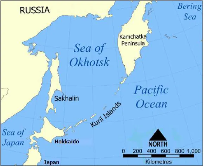
The price to produce energy is on the rise; as a consequence, there is a growing demand for the development of new energy resources. Developers are examining non-hospitable areas such as ice covered polar oceans, which occupy approximately 7 % of the total ocean area on Earth (Wang, 2007). The development of oil and gas fields has begun in the Sea of Okhotsk around Sakhalin (shown in Figure I), for example, which is ice covered during the winter season.

Since some of these non-hospitable areas are ice covered all year round, ice class vessels are needed to transport these natural resources. In light of these explorations, the construction of ice class vessels has increased.

1.1 Propellers in Ice

As the production of ice class vessels increases, so does the need for the comprehension of propeller-ice interactions. Presently, the Arctic Shipping Pollution Prevention Regulations (ASPPR), the Finnish-Swedish Ice Class Rules and various classification society rules, are used to make decisions regarding the scantlings, prescribed measurements, of the ice class propellers. These rules were formulated on the basis of a prescribed ice torque depending on the vessel’s particular ice class. However, propeller failures are still being reported.

Problems such as noise, vibration, or even severe bending or failure of the propeller blades can be caused by propeller-ice interactions. A propeller can be stopped during navigation due to ice ramming, maneuvering, or from severe ice loads acting on the propeller. Acquiring more information about propeller-ice interaction can give us more insight on how to make better decisions regarding propeller scantlings and performance (Wang, 2007).

2.0 Experiment

Model scale propeller experiments in the ice tank can provide essential information to explain a mechanism of propeller-ice interaction and to make the proper estimation of ice loads. Deterministic extreme ice loads on a propeller, play an important role in the choice of the strength of the propeller at the initial design stage and the understanding of the interactions between the propeller and ice during navigation stage (Wang et al., 2005). A podded propulsor is used as the model in this experiment and the ice loads were measured at various locations of the model.

2.1 Podded Propulsor

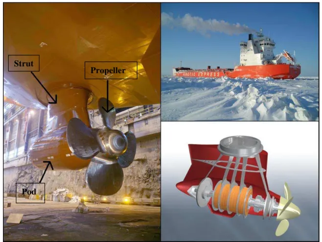
An azimuthing podded propulsor is designed to be able to rotate 360 degrees, by a gearbox within the vessel. Not only is it used as a propulsion system; but it can also be used as a rudderless steering unit. As shown in Figure II, a podded propulsor consists of a strut, a pod with an electric motor, and one or two propellers. An electric motor is contained inside the pod, which receives signals and its power from the ship through the strut.

A podded propulsor system is frequently used on Double Acting Tankers (DAT’s). The principle behind the DAT is that, like most vessels, it travels bow-first on normal open water and thus has a highly hydrodynamic shaped bow and sides (SPG Media Limited, 2009). When it sails in ice however, it travels astern where the reinforced stern hull is used to break the ice.

Strut

Propeller

Pod

Figure II — Full-Scale Podded Propulsion System, Sea Trial and Conceptual Drawing

There are many benefits in the use of a podded propulsor, such as outstanding maneuvering capability through the ability to deliver full thrust in any direction. Also, since the system is somewhat isolated from the hull of the ship, it saves space and reduces noise and vibration (Wang, 2007).

2.2 Test Facilities and Model Ice

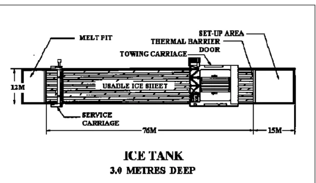
Tests on the model podded propulsor were conducted in the ice tank, (shown in Figure III), at IOT. The ice testing area is 76 meters in length, 12 meters in width, and 3 meters in depth. A thermal door separates a 15-meter long setup area, which allows for equipment preparation while the test ice sheet is prepared. The carriage is designed with a central testing area where the test frame, mounted to the carriage frame, allows the experimental setup to move transversely across the entire width of the tank.

Figure III — Schematic Diagram of Ice Tank

A specifically designed type of ice called EG/AD/S ice was used in these experiments. EG/AD/S ice is a diluted aqueous solution, which is named for its contents: ethylene glycol (EG), aliphatic detergent (AD), and sugar (S). EG/AD/S ice is used because it provides the scaled flexural strengths of columnar sea ice.

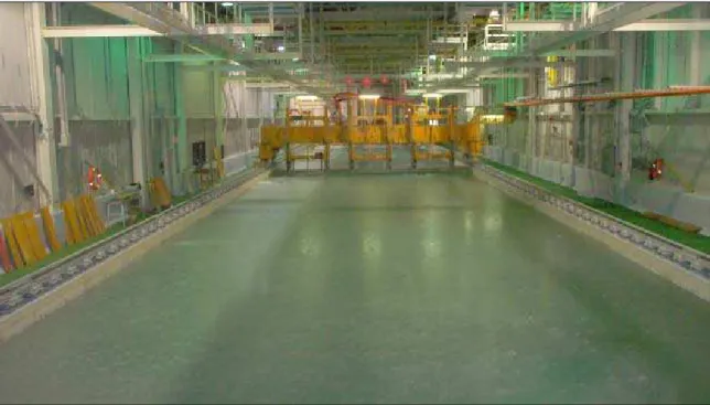
In order to produce the ice for the tests, the growth of the ice sheet is initiated by cooling the tank water and the room to approximately 0 and -20°C, respectively. This is known as cooling. Secondly, a process known as seeding is employed. This involves spraying a warm water mist into the cold air that allows the formation of ice crystals with uniform grain size. Thirdly, the ice is allowed to grow, in a process known as growing, at approximately -20°C until the sheet has reached the desired thickness. Finally, a process known as tempering is employed. The temperature of the tank is raised to above freezing and the ice is then allowed to warm up and soften. This is continued until the target ice strength is reached. Figure IV shows the ice and the ice tank.

Figure IV — Level Ice in Ice Tank

2.3 Dynamometers

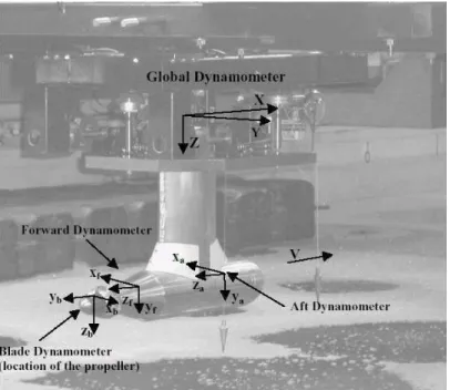
Dynamometers were used to measure the ice loads acting on the different parts of the propulsor during the tests. A blade dynamometer was mounted inside the hub and was attached to one of the blades. This type of dynamometer is capable of measuring forces and moments in six degrees of freedom. Two dynamometers of the same type were attached to the shaft bearings. The global dynamometer was on the top of the pod system, and measured the six degrees of freedom forces and moments in three orthogonal directions (Wang et al., 2005). A strain gauge system mounted on the shaft close to the propeller hub was used to measure shaft torque. Other measurements including carriage velocity, propeller rotating speed (RPS), azimuth angle, and blade angular position were also taken.

2.4 Test Matrix

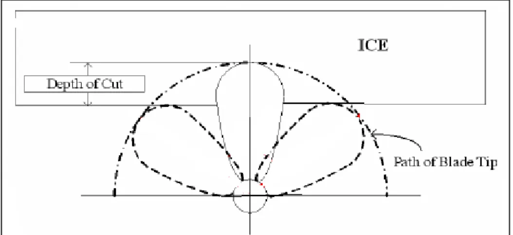
The tests were carried out at different depths of cut (DOC), (the maximum depth that was penetrated by the propeller blade into the ice block (Figure V)), RPS, azimuth angle, and carriage velocity (Vs). They were also carried out at two

different operating conditions, tractor and pusher mode. Table 1 shows the test matrix for the present data analysis in pusher mode from level ice.

Figure V — Depth of Cut

Table 1 – Test Matrix for Pusher Mode

Depth of Cut (DOC) 15 - 20 mm 30 - 43 mm

Azimuthing Angle 6 groups (0, 15, 30, 60, 90, 120)

RPS (/s) 5, 7, 10

Advance Coefficient (J)

Velocity (m/s) 0.2 - 0.6

For data analysis, three different propeller rotational speeds (5, 7, and 10 rps), a range of speed (0.2 – 0.6 m/s), two DOCs (15-20 mm or 30-43mm), and three groups of azimuth angle (0-15, 30-60, or 90-120 degrees), are used.

2.5 Operating Condition

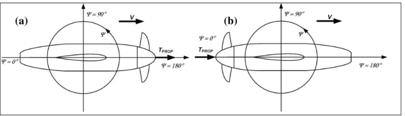
As mentioned previously, a podded propulsor has two different modes; tractor mode and pusher mode. In tractor mode, (also known as puller mode), the propeller is placed in front of the pod and strut so as to give the effect that it is “pulling” the vessel forward (Figure VI (a)). In contrast, in the pusher mode, the propeller is placed at the back of the pod and strut to give the effect that it is “pushing” the vessel forward (Figure VI (b)).

(a) (b)

Figure VI — Comparison of Tractor and Pusher Mode

Tractor mode has been analyzed in propeller-ice interaction studies because it provides uniform ice conditions such as uniform depths of cut. The orientation of the propeller in tractor mode allows it to experience undisturbed ice blocks, which allows for better understanding of the propeller-ice mechanism (Wang, 2007). However, for the pusher mode, this is not the case. Since the propeller is placed at the back of the pod, it may experience broken or damaged ice pieces that are additional loads to the ones experienced from the actual interaction with the ice sheet. For this reason, the analysis of ice loads for the pusher mode can be more complicated.

3.0 Results

The different parameters are recorded and stored as channels. The channels that were used in this experiment are:

• Shaft Speed (RPS) • Blade Angular Position • Azimuth Angle • Motor Current

• Global Fx1 • Blade Dyno Fx • Global Fx2 • Blade Dyno Fy • Global Fy • Blade Dyno Fz • Global Fz1 • Blade Dyno Mx • Global Fz2 • Blade Dyno My • Global Fz3 • Blade Dyno Mz • Aft Dyno Fx • Test Frame Height • Aft Dyno Fy • X inline Load • Aft Dyno Fz • Y Inline Load Cell • Aft Dyno Mx • Carriage Position • Aft Dyno My • Carriage Velocity • Aft Dyno Mz • Carriage Speed • Shaft Torque

Figure VII shows the locations and orientations of the aft, forward, global, and blade dynamometers that measure the data recorded in the channels listed above (Wang et al., 2004).

4.0 Interpretation of Results

In order to gain a complete understanding of the propeller performance in ice, the advance coefficient (J), non-dimensional thrust coefficient (KT), and

non-dimensional torque coefficient (KQ) must be calculated.

4.1 Advance Coefficient (J)

The advance coefficient (J) is the ratio of the speed with which water flows to the propeller or the carriage velocity (Va), to the product of the propeller diameter (D)

and the shaft speed (n) (Harvald, 1991). This is shown is Eq. 1. The diameter of the blade was 0.3 m.

J =

nD

V

(Eq. 1)

4.2 Non-Dimensional Thrust Coefficient (KT)

The non-dimensional thrust coefficient (KT) is the ratio of calculated thrust (T) to

the product of the water density (ρ), the square of the shaft speed (n), and the diameter of the propeller, (D), to an exponent of 4 (Harvald, 1991). This is shown in Eq. 2. The density used for the calculation in these experiments is 1002.5 kg/m3. KT =

D

n

T

ρ

4.3 Non-Dimensional Torque Coefficient (KQ)

The non-dimensional average torque coefficient (KQ) is the ratio of calculated

torque (Q) to the product of the water density (ρ), the square of the shaft speed (n), and the diameter of the propeller, (D), to an exponent of 5. The density is the same value used for the thrust coefficient calculations. This is shown in Eq. 3.

KT =

D

n

Q

ρ

The thrust and torque coefficients of the shaft were used in the present analysis. For the calculation of KT, the axial-component of the forward dyno force is used

for the thrust component. For the calculation of KQ, shaft torque, as mentioned

previously is measured by a strain gauge system mounted on the shaft close to the propeller hub, is used for the torque component. For these channels, as for all the channels, the maximum, minimum, mean and standard deviations were calculated.

4.4 Exceedance Probability

Once the advance coefficient, thrust, and torque coefficients are calculated, the data can be analyzed and interpreted with the additional calculation of exceedance probability. As one of the extreme probability schemes, the Gumbel equation is used (Eq. 4).

(Eq. 4) F(x) = exp[−exp(−x)]

In order to use this equation, it must be assumed that all events are independent and identically distributed random quantities (iid). This can be used to explain propeller-ice interactions, since in an actual scenario, especially in pusher mode, the interactions will not occur continuously. Also, propellers will more often experience ice pieces (pack ice) than level ice.

For the extreme probability method, the only region of interest is the tail of the probability distribution and it may follow an exponential or double exponential form of the Gumbel distribution. In order to use the extreme statistics, the minimum value data sets were ranked in ascending order, while the maximum value data sets were ranked in descending order (Wang et al., 2005).

The Weibull plotting position, [i/(n+1)], was used and double exponential form was used for the tail distribution. Therefore, the exceedance probability was defined as a double logarithm. In the Weibull plotting, n is the total number of

5.0 Data Analysis

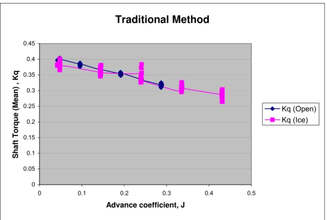
In order to fully gain an understanding of the ice loads on the propeller in pusher mode, the data had to be analyzed differently than traditional propeller performance analysis. The traditional way of representing ice loads is to use the ice loads experienced in open water situations, (no ice), to calculate KQ and J, as

shown in Figure VIII. This is not a good representation of ice loads in pusher mode because it uses the mean values of the parameters used. In order to get a true sense of the interactions, minimum and maximum values should be explored.

Two ways of representing this data for analysis are the blade angular position method and revolution method. For the blade angular positions method, the ice loads are calculated at each individual angle as the propeller rotations. This is done to indentify exactly where the propeller-ice interaction occurs. For the revolutions method, the ice loads experienced by the propeller after each full rotation are calculated. This allows us to identify the maximum ice load at each revolution. The raw data recorded during each run is stored in a database where it can be easily accessed. In order to do the analysis of the aforementioned parameters, a program named Sweet was used.

Traditional Method

Shaft Torque (Mean) , Kq

Kq (Open) Kq (Ice)

Figure VIII — Mean Shaft Torque versus Advance Coefficient

5.1 Sweet

Sweet (SoftWare Environment for Experimental Technologies) is an environment used to manage the information technology needs of scientific and engineering research organizations (National Research Council Canada, 2005). It was developed as a joint project between the Institute for Information Technology (IIT) and the Institute for Ocean Technology. It was used in this experiment to represent the raw data as either blade angular position or revolutions. The procedure that was used in this analysis is outlined in Appendix A.

5.2 Graphing the Results

The aforementioned exceedance probability can be plotted against the non-dimensional coefficients and one can interpret these graphs to gain more

5.2.1 Depth of Cut

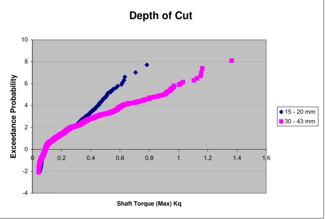
Figure IX is the graphical representation of the relationship between maximum values of shaft torque and exceedance probability in terms of depth of cut. For this analysis, the depths of cut were sorted into two different groups: 15 – 20 mm and 30 – 34 mm. Values from all azimuth angles were used. As you can see from the graph, as the depth of cut increases, the shaft torque also increases at certain exceedance probability. This method can provide a deterministic value of torque corresponding to any design criteria. It is noted that if we assumed that the period of data acquisition is one year, than the exceedance probability for a 100-year load is to be 4.6. The shaft torque coefficients for 15 – 20 mm DOC and 30 – 43 mm DOC for the 100-year load are 0.48 and 0.79, respectively.

Depth of Cut

Shaft Torque (Max) Kq

Exceedance Probability

15 - 20 mm 30 - 43 mm

Figure IX — Graphical Representation of Shaft Torque (Max) versus Exceedance Probability in terms of DOC

5.2.2 Azimuth Angle

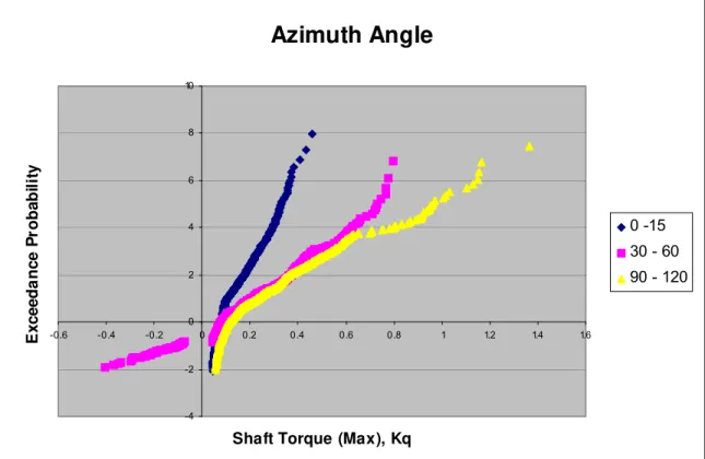
The relationship between the maximum shaft torque and the exceedance probability in terms of azimuthing angle is shown in Figure X. There were 6 azimuth angles that were tested. They were sorted into 3 groups, which are 0 – 15, 30 – 60, and 90 – 120 degrees. As you can see from the graph, as the azimuth angle increases, the maximum shaft thrust also increases, the same scenario as with depth of cut. This occurs because as the azimuth angle increases from 0 degrees, the propeller experiences more contact with the undisturbed ice sheet.

Azimuth Angle

Shaft Torque (Max), Kq

E xce ed a n ce P ro b ab il it y 0 -15 30 - 60 90 - 120

Figure X — Graphical Representation of Shaft Torque (Max) versus Exceedance Probability in Terms of Azimuth Angle

5.2.3 Advance Coefficient

Figure XI shows the relationship between the maximum shaft torque and the exceedance probability in terms of only the advance coefficient. In this situation, the data that is used is at an azimuth angle of 0 – 15 degrees and a DOC of 30 – 43 mm. As can be shown from the graph, as the advance coefficient increases, the shaft torque also increases. This can be attributed to the fact that J increases as the carriage velocity increases and keeping the shaft speed and diameter constant.

Advance Coefficient

Shaft Torque (Max), Kq

Exceedance Probability

J1 (0< - 0.2) J2 (0.2 - 0.4) J3 (0.4<)

Figure XI — Graphical Representation of Maximum Shaft Torque versus Exceedance Probability in Terms of Advance Coefficient

6.0 Conclusion

For better understanding of the ice loads experienced in pusher mode, different methods (revolution method with extreme probability) than the traditional method used for open water are used for data analysis. As previously mentioned, mean values for these parameters do not give a precise representation of the ice loads because of the un-uniform conditions experienced during pusher mode.

Using the revolution method, it is able to identify the maximum ice loads experienced by the prop at each revolution. After setting an appropriate return period of the probability, deterministic values of the ice loads, (here we used shaft torque), can be provided depending on the design criteria (such as a 100-year load). Revolution method was implemented in Sweet and it was verified. This method can reduce the gap of the knowledge of propeller-ice interaction and help better decisions regarding the scantlings of propellers.

7.0 References

Harvald, S. A. (1991). Resistance and Propulsion of Ships. Malabar, Florida:

Kreiger Publishing Company.

Wang, J., Akinturk, A., Foster, W., Jones, S. J., Bose, N. (2004). An

Experimental Model for Ice Performance of Podded Propellers. Proc. Of

the 27th American Towing Tank Conference, August 6-7, St. John’s, Canada

Wang, J., Akinturk, A., Jones, S. J., Bose, N. (2005). Model Podded Propeller-Ice Interaction in extreme Conditions using a Probabilistic Model. Proc. of

the 7th Canadian Marine Hydromechanics and Structures Conference, Sept. 21-22, 2005, Halifax, Canada

National Research Council Canada. (2005, February 21). About Us. Retrieved

March 2009, from NRC-CNRC Institute of Ocean Technology: iot-ito.nrc-cnrc.gc.ca/about_e.html

SPG Media Limited. (2009). Tempera - Double Acting Tanker. Retrieved March

2009, from Ship Technology: www.ship-technology.com/projects/tempera/

Wang, J. (2007). Prediction of Propeller Performance on a Model Podded Propulsor in Ice (Propeller-Ice Interaction). Ph.D. Thesis, Memorial

Univeristy of Newfoundland, Canada

Wikipedia. (2007, 11 05). Sakhalin. Retrieved February 2009, from Wikipedia:

http://en.wikipedia.org/wiki/File:Sea_of_Okhotsk_map_ZI-2b.PNG

Appendix A

Initial Setup

1. Select ‘File’, then ‘Open Run Set File’ 2. Select ‘Pusher Mode analysis.py’ 3. Select ‘New Run’

4. Select desired run file from Ice Database (I:\) 5. Choose ‘bsg_custom.py’ for Custom Processor 6. Select ‘Perform Taring’ Check box

For Revolution Analysis:

1. Change Project Title to ‘Revolution Analysis’

2. Write the names of the desired channels that are wanted to be displayed in Displayed Channels or write the unwanted channels in Excluded Channels 3. Choose ‘make_prop_revolution’ from the drop down box in the Custom

Processor parameter

4. Write ‘Prop_Revol.’ in Bin Channel parameter 5. Use ‘BinSize’ as Bin usage parameter

6. Use 1.0 for Bin Size

7. Use 360 for number of bins

8. For future runs, if same segments are desired for use, use Reanalysis mode.

For Blade Angular Position Analysis:

1. Change Project Title to ‘Blade Angular Position Analysis’

2. Write the names of the desired channels that are wanted to be displayed in Displayed Channels or write the unwanted channels in Excluded Channels 3. Choose ‘make_blade_position’ from the drop down box in the Custom

Processor parameter

4. Write ‘Assumed Blade Angular Position’ in Bin Channel parameter 5. Use ‘Number of bins’ as Bin usage parameter

6. Use 1.0 for Bin Size