Evaluation of Airborne Sound Insulation in Terms of Speech Intelligibility

(1)

Publisher’s version / Version de l'éditeur:

https://publications-cnrc.canada.ca/fra/droits

L’accès à ce site Web et l’utilisation de son contenu sont assujettis aux conditions présentées dans le site

Research Report (National Research Council of Canada. Institute for Research in

Construction), 2007-02-01

READ THESE TERMS AND CONDITIONS CAREFULLY BEFORE USING THIS WEBSITE.

https://nrc-publications.canada.ca/eng/copyright

NRC Publications Archive Record / Notice des Archives des publications du CNRC :

https://nrc-publications.canada.ca/eng/view/object/?id=1bddec5e-b73b-41b0-bd7a-ae4c1c00c5e5 https://publications-cnrc.canada.ca/fra/voir/objet/?id=1bddec5e-b73b-41b0-bd7a-ae4c1c00c5e5

NRC Publications Archive

Archives des publications du CNRC

For the publisher’s version, please access the DOI link below./ Pour consulter la version de l’éditeur, utilisez le lien DOI ci-dessous.

https://doi.org/10.4224/20377977

Access and use of this website and the material on it are subject to the Terms and Conditions set forth at

Evaluation of Airborne Sound Insulation in Terms of Speech

Intelligibility

(2)

http://irc.nrc-cnrc.gc.ca

E v a l u a t i o n o f A i r b o r n e S o u n d I n s u l a t i o n i n

T e r m s o f S p e e c h I n t e l l i g i b i l i t y

I R C - R R - 2 2 8

P a r k , H . K . ; B r a d l e y , J . S . ; G o v e r , B . N .

J u n e 2 0 0 7

The material in this document is covered by the provisions of the Copyright Act, by Canadian laws, policies, regulations and international agreements. Such provisions serve to identify the information source and, in specific instances, to prohibit reproduction of materials without written permission. For more information visit http://laws.justice.gc.ca/en/showtdm/cs/C-42

Les renseignements dans ce document sont protégés par la Loi sur le droit d'auteur, par les lois, les politiques et les règlements du Canada et des accords internationaux. Ces dispositions permettent d'identifier la source de l'information et, dans certains cas, d'interdire la copie de documents sans permission écrite. Pour obtenir de plus amples renseignements : http://lois.justice.gc.ca/fr/showtdm/cs/C-42

(3)

Evaluation of Airborne Sound Insulation in Terms of

Speech Intelligibility

Hyeon Ku Park, John S. Bradley and Bradford N. Gover

IRC Research Report, IRC RR-228

February 2007

(4)

Summary

This report gives the results of new listening tests to evaluate various airborne sound

insulation ratings in terms of the intelligibility of transmitted speech. These subjective

evaluations of sound insulation ratings are a first experiment of several intended to

validate existing sound insulation ratings and investigate possible improvements.

In these experiments listeners heard test sentences played through 20 different simulated

walls in the presence of a constant low-level ambient noise. The mean intelligibility

scores from 15 subjects, each listening to 5 different sentences for each wall, were used

to test the suitability and accuracy of various sound insulation rating measures for speech

sounds.

The results show that the ISO standard Weighted Sound Reduction Index (R

w

) and

ASTM Sound Transmission Class (STC) ratings were not good predictors of the

intelligibility of the transmitted speech sounds. However, measures that are intended to

be indicators of the intelligibility of speech, such as the Articulation Index (AI), the

Speech Intelligibility Index (SII), and the Articulation Class (AC), were much more

strongly related with the mean intelligibility scores. In these experiments the variations in

these quantities only related to variations in the transmission characteristics of the

simulated walls because the speech source level and the ambient noise level were not

varied.

When various other types of possible sound insulation ratings were considered, those that

were based on arithmetic averaging of decibel values were more successful than those

based on energy summation of the information over various frequency bands. This is

expected, because the well-established AI measure is based on this concept.

Measures that limit the included frequency bands or weight their importance according to

their influence on the intelligibility of speech were also seen to be better predictors of the

intelligibility of the transmitted speech. Two more successful approaches included an

arithmetic average of transmission loss values over speech frequencies and a new speech

shaped spectrum weighting for the ISO R

w

procedure.

Future experiments will evaluate sound insulation ratings using other types of sounds and

subjective responses.

(5)

Acknowledgements

The authors would like to thank Marina Apfel (Fachhochschule für Technik, Stuttgart) and Stephanie Loiselle (University of Ottawa) for carrying out the listening tests. The authors also very much appreciated the NRC employees who volunteered to be subjects and made this work possible.

(6)

1. Introduction

Airborne sound transmission through partitions separating dwellings and other spaces is

measured over a range of frequencies in standardized tests. In North America the ASTM E90 [1] procedure is used in the laboratory and the ASTM E336 [2] procedure is used in field situations. In most other countries the ISO 140 procedures [3] are usually followed to measure airborne sound transmission through walls and floors. These procedures are all very similar and include single number ratings to reduce the results at a number of frequencies to a single numerical value. The STC (Sound Transmission Class) from the ASTM E413 standard [4] and the Rw (Weighted

Sound Reduction Index) from the ISO 717-1 standard [5] are quite similar in their derivation and

are widely used to specify the required sound insulation in various situations such as between homes.

It is important that ratings accurately indicate the perceived rank ordering of the sound insulation of different partitions so that they can be designed to maximize occupant satisfaction [6-10]. However, STC and Rw are not based on the results of controlled listening tests and there are

studies that suggest they are not necessarily the most accurate indicators of human perceptions. For example, Tachibana in Japan [11] has carried out studies that suggest a simple arithmetic average of the sound transmission values in each frequency band would be better. Recent work at NRC-IRC [12] has also indicated that listeners’ responses to speech sounds are well related to simple arithmetic average type measures. There is also much controversy over the use of the ‘8-dB rule’ included in the ASTM STC rating but is not in the ISO procedures [13, 14].

1.1 Standard Sound Insulation Measures

The ASTM procedure described in ASTM E90 for laboratory tests and in ASTM E336 for field measurements are most commonly used in North America to measure the airborne sound insulation of walls and floors. They specify the measurement of sound transmission loss in 1/3-octave bands from 125 Hz to 4k Hz. The ASTM E413 standard describes how to determine the STC (Sound Transmission Class) single number rating from the16 measured 1/3-octave band sound transmission loss values. STC is obtained by comparing a rating contour with the measured sound transmission loss values. The rating curve is systematically shifted to higher transmission loss values until one of two criteria is exceeded. The differences from the rating curve down to the measured transmission loss values are called deficiencies. The first criterion is that the sum of all deficiencies summed over the 16 1/3-octave bands must not exceed 32 dB. The second criteria is that the deficiency in any one band must not exceed 8 dB. This latter criterion is to avoid having particularly strong transmitted sound in a particular 1/3-octave band.

In most other areas of the world, the ISO 140 procedure [3] is used to measure airborne sound transmission loss. The procedure is very similar to the ASTM procedures except that

measurements are made for the 16 octave bands from 100 Hz to 3.15 kHz. The measured 1/3-octave band sound transmission loss values are used to derive a single number rating of the sound insulation, the Weighted Sound Reduction Index (Rw) as described in the ISO 717-1 standard. It is

essentially the same as the ASTM procedure for determining the STC rating except there is no 8-dB rule in the ISO 717-1 procedure.

The ISO 717 procedure also includes possible spectrum adaptation terms that are intended to make the ISO procedure more appropriate for rating airborne sound insulation for specific types

(8)

1.2 Measures of Speech Intelligibility

The intelligibility of speech is primarily related to the sound level of the speech relative to the level of interfering noise as measured by various signal-to-noise ratios. As one purpose of walls and floors is to block speech sounds, their success as sound barriers can be measured in terms of the intelligibility of transmitted speech sounds. It is therefore of interest to consider speech intelligibility measures and related quantities as possible correlates of subjective ratings of airborne sound insulation. In this experiment the source speech level and the ambient noise level at the listener’s position were fixed. Therefore the variations in the speech intelligibility measures were only due to the variations in the simulated transmission characteristics of the walls. All of these measures have in common that they are arithmetic averages of decibel values over speech frequency ranges. This approach is derived from the work of French and Steinberg [16] that led to the development of the Articulation Index (AI).

The Articulation Index is calculated as an arithmetic average of the weighted signal-to-noise ratios that are in decibels over the 1/3-octave band frequencies from 200 Hz to 5 kHz. The

included frequencies are those important for speech intelligibility. The frequency weightings have been determined to indicate the relative importance of each included frequency band to the overall intelligibility of speech. The range of included signal-to-noise ratios is limited to those thought to relate to between 0% and 100% intelligibility and the weighted average of the signal-to-noise values over frequency is transformed to a number between 0 and 1.

The Speech Intelligibility Index (SII) [17] is essentially a newer version of the Articulation Index [18]. It has modified frequency weightings and is calculated over the 1/3-octave bands from 160 Hz to 8k Hz. SII values are also between 0 and 1 but tend to be slightly larger than the

corresponding AI values.

The same frequency weightings as used in the AI measure have been used to create the

Articulation Class (AC) described in the ASTM E1110-01 standard [19]. The Articulation Class is simply a weighted sum of attenuations over the same frequency range as the AI measure, that is 200 Hz to 5k Hz. Of course, the attenuations could be sound transmission loss values and the AC measure could be used as a single number sound insulation rating.

1.3 Previous Research Results

Vian et al. [20] conducted subjective listening tests in the laboratory to assess the adequacy of a French rating method for sound isolation in buildings based on an A-weighted level difference using a pink noise source. They concluded that annoyance responses were most strongly correlated with A-weighted level differences limited to include information only in the 1/3-octave bands from 125 Hz to 4k Hz. Annoyance responses were less strongly correlated with A-weighted level differences for a broader range of frequencies and not significantly related to the un-weighted sound pressure levels of the transmitted music sounds. Annoyance responses were also related to differences among music samples and to the slope of the simulated transmission loss versus frequency curve. The slope between 100 Hz and 1k Hz was said to be the most important portion of the sound insulation curve. Music samples that included words in the language of the listeners (French) were more annoying than those they did not understand (English). The tests included listening to the 144 combinations of 12 different pieces of music and 12 simulated transmission loss versus frequency curves. The simulated sound transmission loss curves were constructed to systematically vary key features such as the slope and the location of coincidence dips and did not exactly model the characteristics of real walls.

Tachibana et al. [11] performed an experiment to establish a rating method for airborne sound insulation in buildings through loudness evaluations. He used eleven models to represent sound insulation characteristics and three models for the noises incident on the walls, which were

(9)

electronically synthesized by filtering the output of a random noise generator. The various test sounds were modified to simulate transmission through the 11 different wall models and were presented to subjects from a loudspeaker in an anechoic room. Using the method of adjustment, subjects determined when reference sounds were equally loud to the sounds transmitted through the simulated walls. Although Steven’s Perceived Level (PL) was well correlated with the loudness judgments, the arithmetic mean of the transmitted sounds from 63 to 4k Hz was judged to be the most successful predictor of the loudness responses.

Recent work at IRC [12], evaluated a number of measures for rating the speech security of meeting rooms, where speech security indicates very high levels of speech privacy. Although AI and SII were generally good predictors of speech intelligibility, they were less successful at very low levels of intelligibility because both measures approach asymptotically to 0 for such

situations. Frequency-weighted signal-to-noise ratios were found to be more widely applicable and could be used to assess conditions where speech was just audible but not intelligible. An SII weighted signal-to-noise ratio (SNRsii22) was found to be best correlated with intelligibility scores and subjective evaluations of the threshold of intelligibility. However, a uniform weighted signal-to-noise ratio, (SNRuni32) was better correlated with perceptions of the threshold of audibility of the speech. The SNRuni32 measure was judged to be the best measure for predicting both the audibility and the intelligibility of speech transmitted through several

simulated walls.

1.4 The New Work

Because of the lack of previous research to validate the subjective relevance of various standard airborne sound insulation measures, these initial controlled listening tests were carried out in terms of subjective ratings of the intelligibility of transmitted speech. This is an ideal subjective rating to consider first because quite precise results can be obtained and other types of subjective ratings can be considered later if warranted.

Subjects listened to speech modified to simulate the effects of transmission through 20 different walls with a wide range of sound transmission characteristics. The speech was played to subjects from one set of loudspeakers in a sound isolated listening room. At the same time, a constant simulated ambient noise was played from a second set of loudspeakers. Speech intelligibility scores were derived from the fraction of the words correctly understood for speech through each simulated wall.

The standard sound transmission measures, STC and Rw, were first evaluated as well as a number

of variations of these measures. Other insulation ratings related to various speech intelligibility measures using arithmetic averaging of the transmitted sounds in various frequency bands were also evaluated. This included systematic evaluations of the importance of various frequencies to achieving a more precise rating of the sound insulation.

The results suggest which are the more accurate predictors of the intelligibility of transmitted speech through various common types of walls.

(10)

2. Experimental Method

2. 1 Test Facility

All tests were conducted in the Room Acoustics Test Space in Building M-59 at the National Research Council. This is a room measuring 9.2 m long by 4.7 m wide by 3.6 m high, which is constructed from concrete. The room is not connected to the building, and is resting on springs for vibration isolation. Sounds existing outside the room, therefore, are largely isolated from penetrating within. For the present study, the interior walls of the room were lined with 10 cm-thick absorbing foam, covered by curtains. There was a conventional T-bar ceiling with 25 mm-thick glass fibre ceiling tiles installed, and the floor was covered with carpet. This interior treatment yielded a quite “dead” space, enabling the experimenters to completely control the sounds within the room. The background noise level in the room was about 11.6 dBA (measured with the sound simulation system turned off).

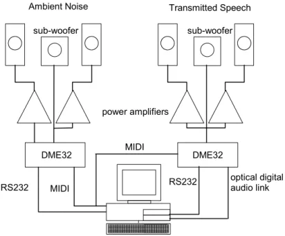
The test speech was played over loudspeakers positioned at the front of the room. The background noise was played over another set of loudspeakers positioned above the ceiling, directly above the subject. Figure 1 shows a diagram of the setup.

Ambient noise loudspeakers Ceiling Curtain Transmitted speech loudspeakers Foam Listener

Figure 1. Schematic of cross-section through Room Acoustics Test Space showing the location of the listener and the loudspeakers used to generate the test sound fields.

A block diagram of the electro-acoustic system used to produce the test sounds is shown in Figure 2. The two blocks labelled ‘DME32’ are Yamaha Digital Mixing Engines, which are highly flexible signal processing boxes, able to perform the functions of many interconnected devices such as equalizers, filters, oscillators, etc. The outputs of the DME32s run via the power amplifiers into high-quality loudspeaker systems (Paradigm Compact Monitors, Paradigm PW sub-woofers). One component in each DME32 was initially configured under computer control (via the RS232 interface) to equalize the playback path through the power amplifiers and loudspeakers to be flat at the position of the listener’s head (± 1 dB from 60 to 12000 Hz). The background noises for the test sound fields were generated by the internal oscillator of one of the DME32 units that can generate broadband noise. This same unit shaped the spectrum and adjusted the level as desired. One channel of the noise output was delayed by 300 ms relative to the other to avoid the two noise signals arriving approximately coherently at the listener’s position. This would avoid any unnatural perceptual effects when the listener moved their head. The speech sounds were generated from playback of anechoically-recorded source material stored on the computer in 16-bit, 44.1 kHz wav-file format. The output of the sound card ran into the second DME32, which performed the necessary equalization and level adjustment. The required

(11)

equalization to simulate the transmission loss of each of the 20 walls were stored in separate ‘scenes’, which can be selected from the computer over the MIDI interface.

Ambient Noise _{Transmitted Speech}

sub-woofer sub-woofer

power amplifiers

DME32 MIDI DME32

MIDI

optical digital audio link

RS232 RS232

Figure 2. Block diagram of the computer controlled electro-acoustic system used to create the test sounds.

2.2 Simulated Walls

First, walls were selected that included the widest possible range of STC ratings. Of these walls some were selected to provide an even distribution of values from very low to very high STC ratings. When speech, at a fixed level, was played through these simulated walls, some of the walls led to 100% speech intelligibility scores while others always led to 0% intelligibility. These walls with either very low or very high STC values were then eliminated. This led to the selection of 20 walls with STC ratings evenly distributed from STC 34 to STC 58 that were expected to lead to intelligibility scores between 0% and 100%.

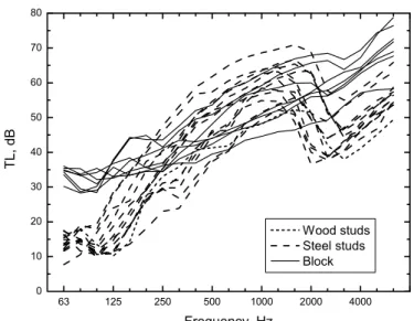
The sound transmission loss versus frequency curves for the 20 selected walls are shown in Figure 3. The shapes and overall levels of the transmission loss values vary considerably and the data represent a broad range of real walls. The walls containing wood studs, steel studs and concrete blocks are separately identified in this figure and are seen to have quite different characteristics.

(12)

63 125 250 500 1000 2000 4000 0 10 20 30 40 50 60 70 80 TL, dB Frequency, Hz Wood studs Steel studs Block

Figure 3. Sound Transmission loss versus 1/3-octave band frequency for the 20 walls simulated in the listening tests, where those containing wood studs, steel studs and concrete blocks are

separately identified.

Table 1 provides a summary of the wall constructions and their STC and Rw ratings. The walls

are common constructions in North America with STC ratings varying from a quite modest (STC 34) to a very good sound insulation rating (STC 58).

No. Descriptor STC rating Rw rating 1 G13_GFB90_WS89_G13 34 37 2 G13_SS65_G13 34 33 3 G16_SS65_G16 35 37 4 G16_SS90_G16 36 37 5 G16_SS90_G16 37 36 6 G13_GFB90_SS90_G13 39 41 7 G16_SS40_AIR10_SS40_G16 39 38 8 G13_GFB90_SS90_G13 40 42 9 G13_GFB65_SS65_G13 43 43 10 BLK90 44 44 11 G16_MFB40_SS90_G16 45 45 12 BLK140 47 47 13 G16_GFB90_SS90_G16 47 45 14 BLK190_PAI 48 48 15 G16_BLK190_G16 49 50 16 BLK190 50 50 17 G16_GFB90_SS90_2G16 52 50 18 2G13_GFB90_SS90_2G13 53 52 19 PAI_BLK140_WFUR40_GFB38_G13 56 55 20 PAI_BLK140_GFB38_WFUR40_G13 58 56

Table 1. Summary of simulated wall constructions with their STC and Rw ratings.

The descriptor codes are explained in Table 2. For example, wall number 17, which is described as, G16_GFB90_SS90_2G16, indicates the various layers of the construction from one side to the

(13)

other. In this case the construction includes: 16 mm gypsum board (G16), 90 mm glass fibre batts (GFB90), 90 mm steel studs (SS90), and 2 layers of 16 mm gypsum board (2G16).

Descriptor Explanation Descriptor Explanation

AIR Air space PAI Paint

BLK Concrete block SS Steel stud

G Gypsum board WFUR Wood furring

GFB Glass fibre batt WS Wood stud

MFB Mineral fibre batt

Table 2. Explanation of symbols used to describe the simulated wall constructions.

2.3 Speech and Noise Test Sounds

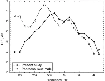
The speech tests used the Harvard sentences [21]. These are phonetically balanced English sentences with content that is of low predictability. This is important to minimize the effects of guessing. The sentences were all recorded by the same clear speaking male talker. Figure 4 shows a sample of the speech spectrum used in the tests compared with that of Pearsons’ result for loud speech [22]. 125 250 500 1k 2k 4k 40 45 50 55 60 65 70 75 SPL, dB Frequency, Hz Present study

Pearsons, loud male

Figure 4. Comparison of the spectrum of the speech used in the current tests with that from Pearsons for loud male speech [22].

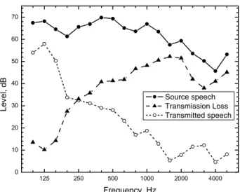
The speech was played, at a fixed source level, through 1/3-octave band equalizers set to represent the transmission loss characteristics of the 20 different walls listed in Table 1. Speech sounds were presented from loudspeakers behind a curtain in front of the subjects. Figure 5 gives an example of the spectrum of the speech before and after modification to represent transmission through a wall.

The noise was played from the loudspeakers above the ceiling. It had a -5 dB/octave spectrum shape and was intended to approximate typical indoor ventilation noise. The overall level of the noise was 35 dBA and was the same for all simulated walls and test sentences.

(14)

125 250 500 1000 2000 4000 0 10 20 30 40 50 60 70 Le v e l, d B Frequency, Hz Source speech Transmission Loss Transmitted speech

Figure 5. Spectrum of speech before and after transmission, as well as the wall transmission loss (TL).

2.4 Subjects

Subjects were all NRC employees who volunteered to do the test. They were not paid or rewarded in any way and the experimental protocol was approved by the NRC Research Ethics Board (protocol 2006-27). A total of 15 subjects completed the test.

All subjects were first given a hearing sensitivity test. Their pure tone average (PTA) hearing levels varied from –1.7 dB to 9.2 dB (averaged over the test frequencies 500, 1k and 2k Hz). The average measured hearing levels (HL) of the 15 subjects are compared with various percentiles of the expected distribution of a population of normal hearing listeners from ISO 7029 1984 [23] in Figure 6. The subjects had, on average, hearing levels approximating the 50th percentile of the ISO results. The results in Figure 6 indicate values that are approximately representative of the average of normal hearing listeners.

-10 0 10 20 30 40 50 125 250 500 750 1k 1.5k 2k 3k 4k 6k 8k Frequency, Hz HL, dB Mean HL 90% 75% 50% 25% 10%

Figure 6. Average Hearing Level (HL) for the 15 subjects compared with the ISO percentiles for a normal population. (The percentile values at 750 Hz are interpolations of the ISO data).

2.3 Test Procedure and Analyses

To familiarize subjects with the types of sounds they would hear, they first listened to 10 different test sentences played through 10 different simulated walls that varied from very low to very high

(15)

STC rating. They were told that the practice sentences were representative of the full range of conditions that they would hear in the full test.

In the full test, listeners heard 5 different Harvard sentences through each of the 20 simulated walls for a total of 100 sentences. The order of the sentences and of the walls was randomized so that subjects heard conditions in one of three different randomized orders. Only the simulated transmission characteristics of the walls were varied. The effective speech source level and the ambient noise level at the listener’s position remained constant through the tests.

The results were analyzed in terms of the average intelligibility scores for all listeners and all test sentences for each wall. That is, each average speech intelligibility score was an average of scores for 5 sentences x 15 subjects or 75 different test scores.

Most of the following analyses consist of plots of the mean speech intelligibility scores versus some sound insulation rating measure such as STC. To test the strength of the correlation between the intelligibility scores and the sound insulation ratings to types of best fit regression lines were fitted to the results. For all analyses 3rd order polynomials were fitted and the related R2 values were calculated. In most cases Boltzmann equations were also fitted and the related R2 values calculated. The Boltzmann equation is given by the following,

2 / ) ( 2 1 0

1 e

A

y

_x _x _dx

+

−

=

₋ (1) where, A1= y-value for x= -∞ (0% or 100%) A2= y-value for x= +∞ (0% or 100%)

x0= x-value of mean y-value, that is the x-value when y=50% in our case

dx = relates to the slope of the mid-part of the regression line

The Boltzmann equation better fits the expected speech intelligibility responses because the fitted Boltzmann equations were forced to approach asymptotically to 0% and 100%

intelligibility for the extreme values of the sound insulation measure (i.e. the A1 and A2 values

were set to either 0 or 100). Although the 3rd order polynomial fits do not fit the expected variation of the scores as well for very high and very low values, they are often a good indicator of the approximate relationship. This is especially true when the related R2 values are relatively high. The R2 values for both the Boltzmann equation fits and the 3rd order polynomial fits have been included to demonstrate those conditions where the two approaches give approximately the same results. In many situations 3rd order polynomial fits can be used to more quickly obtain approximate indications of the strengths of the various relationships.

All of the results presented in this report were statistically significant for at least a probability of occurring by chance of p < 0.05. Since there are always 20 data points and the same format of regression equation, the significance is simply related to the R2 value. For any R2 value in this report ≥ 0.317 the relationship can be said to be highly significant (p <0.01).

(16)

3. Results

3.1 Evaluation of Standard Sound Insulation Measures

Figure 7 plots the STC ratings of the simulated walls and the mean intelligibility scores (with associated standard errors) versus the wall number. The walls are in order of increasing STC rating. However, it is clear that this order does not correspond to decreasing speech intelligibility.

1 6 11 16 30 40 50 60 STC SI, % Wall STC 20 0 20 40 60 80 100 S p e e c h Inte llig ibi lity , %

Figure 7. Mean speech intelligibility scores with error bars indicating ± 1 standard deviation and

Sound Transmission Class (STC) versus wall number.

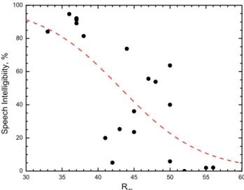
Figure 8 plots the same mean intelligibility scores versus STC value of the simulated walls. As expected from the results of Figure 7, the intelligibility scores are not well correlated with the STC values and STC is not seen to be a good predictor of the intelligibility of the transmitted speech. The regression line on this and subsequent plots is a Boltzmann equation which was forced to asymptotically approach 0% and 100% intelligibility at the two extremes as would be expected for intelligibility scores.

30 35 40 45 50 55 60 0 20 40 60 80 100 Speech I n tell igi b iity , % STC

Figure 8. Speech intelligibility scores versus STC ratings of the simulated walls. (3rd order polynomial fit R2 = 0.583, Boltzmann equation R2= 0.510).

Figure 9 plots mean intelligibility scores versus values of the standard Rw rating for the simulated

walls. The scatter is similar to that for the STC ratings in Figure 8. This is not surprising because of the similarity of the STC and Rw procedures. Figures 8 and 9 indicate that neither STC nor Rw,

(17)

values, in their currently standardised forms, is a good predictor of the intelligibility of the transmitted speech. 30 35 40 45 50 55 60 0 20 40 60 80 100 Sp eech In tell igi b iity, % R_w

Figure 9. Speech intelligibility scores versus Rw ratings of the simulated walls.

(3rd order polynomial fit R2 = 0.580, Boltzmann equation R2= 0.542).

3.2 Evaluation of Speech Intelligibility Measures

This section presents the results relating the mean intelligibility scores to various speech intelligibility type measures. Figure 10 plots the mean intelligibility scores versus values of the Articulation Index (AI). The results in Figure 10 have higher R2 values than those in the previous section indicating that the AI is a better predictor of the intelligibility of the transmitted speech. This is to be expected because there was considerable research effort over many years [16] to develop the AI for the purpose of predicting expected speech intelligibility.

0.00 0.05 0.10 0.15 0.20 0.25 0 20 40 60 80 100 S p e e ch Int e lligib iity, % AI

(18)

0.00 0.05 0.10 0.15 0.20 0.25 0.30 0.35 0 20 40 60 80 100 S pee ch In tell igibii ty, % SII

Figure 11. Speech intelligibility scores versus SII ratings of the test conditions. (3rd order polynomial fit R2 = 0.909, Boltzmann equation R2= 0.899).

Figure 12, plots the mean intelligibility scores versus values of an AI-weighted signal-to-noise ratio (SNRai) [12]. The frequency weightings are those from the AI measure [18] and the frequencies from 200 Hz to 5 kHz are included in calculating an arithmetic average of the weighted 1/3-octave band signal-to-noise ratios.

-40 -35 -30 -25 -20 -15 0 20 40 60 80 100 Spe e ch Inte lligibii ty, % SNR_ai, dB

Figure 12. Speech intelligibility scores versus SNRai ratings of the test conditions.

The results in Figure 12 have higher R2 values than those for the standard STC and Rw ratings and

are very similar to those for the AI and SII measures. The intelligibility scores are seen to roughly follow the trend of the best fit Boltzmann regression line shown in the figure.

Figure 13 shows a plot of mean intelligibility scores versus values of the SII-weighted signal-to-noise ratio (SNRsii22) [12]. These results are very similar to those in Figure 12 because the two measures (SNRaiand SNRsii22) are so similar. The R2 values when SNRsii22 is the predictor variable in Figure 13 are slightly higher than those for SNRai in Figure 12. Figure 13 also

includes the best fit regression line to the results in a previous study by Gover and Bradley [12] that agrees well with the new results.

(19)

-25 -20 -15 -10 -5 0 0 20 40 60 80 100 Speech Intellig ibiity, % SNR sii22, dB

Gover & Bradley

Figure 13. Speech intelligibility scores versus SNRsii22 ratings of the test conditions. Solid line

labelled ‘Gover & Bradley’ is from previous experiment[12]. (3rd order polynomial fit R2 =0.912, Boltzmann equation R2=0.913)

Gover and Bradley [12] also related estimates of the onset of intelligibility to SNRsii22 values. For

each wall the fraction of the responses indicating that at least one word was understood were determined. When plotted versus SNRsii22 values the value at which 50% of the subjects could

understand at least one word was defined as the threshold of intelligibility. The intelligibility scores in the current tests were examined to obtain similar estimates of the onset of intelligibility. The fraction of the responses indicating at least one word was understood are plotted versus SNRsii22 values in Figure 14. The solid line is the best fit Boltzmann equation from the previous

study and is seen to be a good fit to the data from the current tests.

-25 -20 -15 -10 -5 0 0.0 0.2 0.4 0.6 0.8 1.0 Fra c ti on a b o v e th re s h ol d of int e lligib ilit y SNR_sii22, dB

Gover and Bradley

Figure 14. Fraction of responses above the threshold of intelligibility versus SNRsii22 ratings of

(20)

-30 -25 -20 -15 -10 -5 0 0 20 40 60 80 100 S p e e ch In te lligibiity, % SNR_uni32, dB

Gover & Bradley

Figure 15. Speech intelligibility scores versus SNRuni32 ratings of the test conditions. Solid line

labelled ‘Gover & Bradley’ is from previous experiment[12]. (3rd order polynomial fit R2 =0.857, Boltzmann equation R2=0.853)

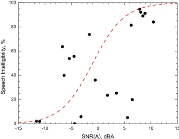
The A-weighted level difference, SNR(A) is sometimes proposed as a simple measure of the intelligibility of speech. Mean speech intelligibility scores are plotted versus the difference between the A-weighted speech level and the A-weighted noise level, SNR(A), in Figure 16. There is clearly not a good relationship with speech intelligibility scores and this result is only just statistically significant (p <.045).

-15 -10 -5 0 5 10 15 0 20 40 60 80 100 S p ee ch I n te llig ibii ty, % SNR(A), dBA

Figure 16. Mean Speech intelligibility scores versus SNR(A) ratings of the test conditions. (3rd order polynomial fit R2 =0.519, Boltzmann equation R2=0.259)

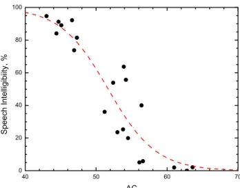
In Figure 17, the mean intelligibility scores are plotted versus values of the Articulation Class (AC) for the simulated walls. Although the R2 values are quite high, intelligibility scores are a little less well correlated with AC values than the other speech intelligibility type measures.

(21)

40 50 60 70 0 20 40 60 80 100 Speech I ntell igi b iity , % AC

Figure 17. Speech intelligibility scores versus the AC ratings of the simulated walls. (3rd order polynomial fit R2 = 0.859, Boltzmann equation R2= 0.856)

The success of the uniform weighted signal-to-noise ratio, SNRuni32, in previous speech security studies [12, 24], suggests that a simple arithmetic average of transmission loss value over speech frequencies should be a reasonably good predictor of the intelligibility of transmitted speech. Values of the Arithmetic Average transmission loss (AA(160-5k)) were calculated over the frequencies from 100 Hz to 5 kHz. Mean intelligibility scores are plotted versus these AA(160-5k) values in Figure 18. The R2 values indicate that this measure is a better predictor of intelligibility scores, than the standard STC and Rw ratings but not quiet as good as the better

speech intelligibility measures. However, this will be seen to be strongly influenced by the frequency bands that are included in calculating the average value.

40 50 60 0 20 40 60 80 100 S p ee ch I n te llig ibi it y , % AA(160-5k), dB

Figure 18. Speech intelligibility scores versus AA(160-5k) ratings of the simulated walls. (3rd order polynomial fit R2 = 0.857, Boltzmann equation R2= 0.853)

(22)

many speech intelligibility measures described in the previous section. Several quantities were investigated that involve energy averaging or energy summation of the information from various frequency bands. In this section these measures are evaluated as predictors of speech

intelligibility scores.

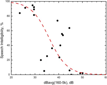
Speech intelligibility scores are plotted versus values of the measure dBavg(160-5k) in Figure 19. The dBavg(160-5k) values are energy averages of the transmission loss values from 160 to 5k Hz.

20 30 40 50 60 0 20 40 60 80 100 Speech Inte lli g ibi ity, % dBavg(160-5k), dB

Figure 19. Speech intelligibility scores versus dBavg(160-5k) ratings of the simulated walls. (3rd order polynomial fit R2 = 0.446, Boltzmann equation R2= 0.523)

STA is an A-weighted sound transmission loss measure [25]. It is calculated by A-weighting and summing the1/3-octave band transmission loss values (from 100 to 4k Hz) on an energy basis as shown in the following equation.

        ⋅ =

∑

= + − k b b b Awt TL 4 100 / ) ( 10 10 17 1 log 10 STA _,_dB₍₂₎

where, Awtb is the A-weighting attenuation in band ‘b’ and TLb is the sound transmission loss in

band ‘b’.

Mean intelligibility scores are plotted versus STA values in Figure 20. Although A-weighting is often used to approximate the response of our hearing system, in this case it does not lead to an improved sound insulation rating measure. It is less well correlated with intelligibility scores than the standard STC and Rw measures.

(23)

30 35 40 45 50 55 60 0 20 40 60 80 100 Speech Int e lli gibii ty , % STA, dB

Figure 20. Speech intelligibility scores versus STA ratings of the simulated walls. (3rd order polynomial fit R2 = 0.513, Boltzmann equation R2= 0.361)

While A-weighting can be thought of as a simple loudness measure, the Zwicker loudness level procedure is intended to give ratings more closely related with loudness judgments. Figure 21 plots mean intelligibility scores versus calculated loudness of the speech transmitted through the simulated walls in Sones. The R2 values below the caption to this figure are very low compared to most of the other measures considered in this report.

0 1 2 3 4 5 0 20 40 60 80 100 S p ee ch I n te llig ibii ty, % Loudness, Sones

Figure 21. Speech intelligibility scores versus loudness ratings in Sones of the speech transmitted through the simulated walls.

(3rd order polynomial fit R2 = 0.473, Boltzmann equation R2= 0.305)

Although some energy summation type measures are somewhat more strongly correlated with intelligibility scores than the standard STC and Rw measures, they are not as well correlated with

(24)

correlations, since the added information does not contain information related to the intelligibility of the transmitted speech. The AI measure includes information in the 1/3-octave bands from 200 Hz to 5 kHz, while the SII measure includes levels from the 160 Hz to the 8 kHz 1/3-octave bands. Neither includes low frequency information unrelated to speech intelligibility.

Figure 22 illustrates the more important frequency bands in this study by showing the results of simple correlations of the intelligibility scores with the transmission loss values in each 1/3-octave band. It is seen that the 1/3-1/3-octave bands from 160 Hz to 2.5 kHz (or maybe 3.15 kHz) yield the highest correlations and hence are most important for predicting intelligibility scores. Lower frequency bands are less important because there is less speech energy in human voices below 160 Hz. The higher frequency bands above 2.5 kHz are less important because little speech energy in this range is effectively transmitted through most walls. This is different to the range of include frequencies in the AI and SII measures that were developed to consider natural

unmodified speech. The severe filtering that results from sound transmission through typical walls removes the significance of these higher frequencies.

63 125 250 500 1k 2k 4k 8k -1.0 -0.8 -0.6 -0.4 -0.2 0.0 Correl a ti on Coeff fi c ient Frequency, Hz

Figure 22, Results of correlations between mean intelligibility scores and individual 1/3-octave band transmission loss values.

Further analyses were carried out to determine the optimum range of frequencies to include when predicting the intelligibility of transmitted speech. These analyses involved recalculation of an Arithmetic Average (AA) transmission loss measure for varied lower and upper included

frequency bands. The previous AA results in Figure 18 were calculated by arithmetical averaging the sound transmission loss values for the frequency bands from 100 to 5k Hz inclusive. In these new analyses the lowest included frequency was systematically increased from 63 Hz to 2000 Hz. In addition, the highest included 1/3-octave band was varied from 200 Hz to 6300 Hz. This resulted in a matrix of correlation coefficients illustrated in Table 3.

(25)

Upper limit frequency, Hz 200 250 315 400 500 630 800 1000 1250 1600 2000 2500 3150 4000 5000 6300 63 -0.36 -0.42 -0.50 -0.58 -0.65 -0.71 -0.75 -0.79 -0.82 -0.85 -0.87 -0.86 -0.84 -0.82 -0.80 -0.79 80 -0.44 -0.50 -0.58 -0.66 -0.72 -0.77 -0.81 -0.84 -0.87 -0.89 -0.90 -0.89 -0.88 -0.86 -0.84 -0.82 100 -0.50 -0.57 -0.64 -0.72 -0.77 -0.82 -0.85 -0.88 -0.90 -0.92 -0.93 -0.92 -0.90 -0.88 -0.87 -0.85 125 -0.60 -0.66 -0.73 -0.79 -0.83 -0.87 -0.89 -0.91 -0.92 -0.94 -0.95 -0.94 -0.93 -0.91 -0.89 -0.88 160 -0.65 -0.71 -0.78 -0.83 -0.87 -0.90 -0.91 -0.92 -0.92 -0.94 -0.95 -0.95 -0.94 -0.93 -0.91 -0.89 200 -0.69 -0.75 -0.81 -0.86 -0.88 -0.90 -0.91 -0.91 -0.91 -0.93 -0.95 -0.96 -0.95 -0.94 -0.92 -0.91 250 -0.79 -0.84 -0.88 -0.89 -0.91 -0.91 -0.90 -0.90 -0.92 -0.94 -0.96 -0.96 -0.95 -0.93 -0.91 315 -0.88 -0.90 -0.91 -0.91 -0.91 -0.90 -0.89 -0.91 -0.94 -0.95 -0.96 -0.95 -0.93 -0.91 400 -0.90 -0.89 -0.90 -0.88 -0.87 -0.86 -0.88 -0.92 -0.95 -0.95 -0.94 -0.93 -0.90 500 -0.87 -0.89 -0.86 -0.84 -0.84 -0.86 -0.91 -0.94 -0.95 -0.93 -0.91 -0.89 630 -0.90 -0.85 -0.83 -0.82 -0.85 -0.91 -0.94 -0.94 -0.92 -0.90 -0.87 800 -0.79 -0.77 -0.78 -0.83 -0.90 -0.93 -0.93 -0.90 -0.87 -0.84 1000 -0.75 -0.77 -0.84 -0.90 -0.92 -0.91 -0.87 -0.83 -0.80 1250 -0.79 -0.86 -0.91 -0.90 -0.87 -0.83 -0.79 -0.75 1600 -0.89 -0.87 -0.85 -0.81 -0.76 -0.72 -0.69 Lower limit frequency, Hz 2000 -0.79 -0.77 -0.72 -0.68 -0.65 -0.62

Table 3. Correlation coefficients from correlating mean intelligibility scores with an arithmetic average transmission loss measure with varied upper and lower included frequencies.

The highest magnitude correlation coefficient has a value of -0.96, which is obtained when the lowest included frequency is increased to about 200 Hz and the highest included frequency is reduced to about 2.5 kHz. As the results in Table 3 illustrate, some other adjacent combinations can result in the same correlation coefficient.

The success of the Arithmetic Average transmission loss with an included frequency range of from 200 Hz to 2.5 kHz is illustrated in Figure 23, which plots speech intelligibility scores versus this measure. The data points follow the best-fit regression line quite closely and quite high R2 values are obtained. It is clear that by eliminating the irrelevant information at lower and higher frequencies better correlations can be achieved with intelligibility scores.

0 20 40 60 80 100 S pee ch In tell igibii ty, %

(26)

matrix of correlation coefficients is given in Table 4. Again the correlation coefficients are largest in magnitude for a restricted range of intermediate frequencies. However, restricting the included lower frequencies is most important for maximizing the magnitudes of the correlation

coefficients. In fact if frequencies from 315 Hz and higher are included, correlation coefficients values are almost always -0.90 or larger in magnitude. This is probably only valid for speech.

Upper limit frequency, Hz

200 250 315 400 500 630 800 1000 1250 1600 2000 2500 3150 4000 5000 6300 63 -0.19 -0.19 -0.19 -0.20 -0.20 -0.20 -0.20 -0.20 -0.20 -0.20 -0.20 -0.20 -0.20 -0.20 -0.20 -0.20 80 -0.27 -0.28 -0.28 -0.29 -0.29 -0.29 -0.29 -0.29 -0.29 -0.29 -0.29 -0.29 -0.29 -0.29 -0.29 -0.29 100 -0.28 -0.28 -0.29 -0.29 -0.29 -0.29 -0.29 -0.29 -0.29 -0.29 -0.29 -0.29 -0.29 -0.29 -0.29 -0.29 125 -0.55 -0.57 -0.58 -0.58 -0.59 -0.59 -0.59 -0.59 -0.59 -0.59 -0.59 -0.59 -0.59 -0.59 -0.59 -0.59 160 -0.64 -0.67 -0.68 -0.69 -0.70 -0.70 -0.71 -0.71 -0.71 -0.71 -0.71 -0.71 -0.71 -0.71 -0.71 -0.71 200 -0.60 -0.62 -0.63 -0.64 -0.65 -0.65 -0.65 -0.65 -0.65 -0.65 -0.65 -0.65 -0.65 -0.66 -0.66 -0.66 250 -0.79 -0.83 -0.84 -0.85 -0.86 -0.86 -0.87 -0.87 -0.87 -0.87 -0.88 -0.88 -0.88 -0.88 -0.88 315 -0.88 -0.90 -0.90 -0.91 -0.91 -0.91 -0.91 -0.91 -0.92 -0.93 -0.92 -0.92 -0.92 -0.92 400 -0.90 -0.90 -0.90 -0.90 -0.90 -0.90 -0.90 -0.94 -0.95 -0.95 -0.94 -0.94 -0.93 500 -0.87 -0.88 -0.88 -0.87 -0.87 -0.88 -0.94 -0.95 -0.94 -0.92 -0.91 -0.91 630 -0.90 -0.88 -0.87 -0.87 -0.88 -0.94 -0.93 -0.90 -0.88 -0.87 -0.87 800 -0.79 -0.78 -0.78 -0.84 -0.91 -0.91 -0.86 -0.83 -0.82 -0.82 1000 -0.75 -0.77 -0.85 -0.89 -0.88 -0.81 -0.79 -0.78 -0.77 1250 -0.79 -0.87 -0.87 -0.84 -0.77 -0.74 -0.73 -0.73 1600 -0.89 -0.84 -0.80 -0.72 -0.69 -0.68 -0.68 Lower limit frequency, Hz 2000 -0.79 -0.75 -0.66 -0.64 -0.63 -0.63

Table 4. Correlation coefficients from correlating mean intelligibility scores with an energy average transmission loss measure with varied upper and lower included frequencies.

3.5 Variations of the STC Rating

This section describes the results of further analyses to investigate the causes of the limitations of the STC measure and how it might be improved. One of the key differences between STC and the Rw is the inclusion of the 8 dB rule in the ASTM measure. The 8 dB rule can lead to some

peculiar results. For example, the transmission loss values of the two walls illustrated in Figure 24 look quite different, but have the same STC 39 rating. This is because the 8 dB rule limits the STC rating. From Table 1, the Rw ratings for these walls are seen to be 38 and 41.

63 125 250 500 1k 2k 4k 0 10 20 30 40 50 60 70 TL, d B Frequency, Hz Wall #6, STC 39, R_w 41, SI 0.20 Wall #7, STC 39, R_w 38, SI 0.81

Figure 24. Comparison of the sound transmission loss versus frequency characteristics of

two walls having the same STC 39 rating.

(27)

Figure 25 illustrates the sound transmission loss values for two walls that seem to have very similar characteristics but have different STC values. Again this is a result of the 8 dB rule and the Rw ratings (that do not include an 8 dB rule) from Table 1 are more similar than the STC

ratings for these walls.

63 125 250 500 1k 2k 4k 0 10 20 30 40 50 60 70 TL, d B Frequency, Hz Wall #6, STC 39, R_w 41, SI 0.20 Wall #9, STC 43, R_w 43, SI 0.25

Figure 25. Comparison of the sound transmission loss versus frequency characteristics of two walls having the different STC ratings (STC 39 and STC 43).

(See Table 1 for description of the constructions of walls #6 and #9).

In both cases the confusing results are due to the application of the 8 dB rule. To test the appropriateness of the 8 dB rule, modified STC values were calculated without an 8 dB rule. Speech intelligibility scores are plotted versus this modified STC value in Figure 26. The modified STC measure without the 8 dB rule is actually better correlated with speech

intelligibility scores than are values of the standard STC measure. The results in Figure 8 for the standard STC measure show R2 values of 0.583 for the 3rd order polynomial fit and 0.510 for the Boltzmann equation fit. Therefore the STC measure is a better predictor of the intelligibility of transmitted speech when the 8 dB rule is removed.

30 35 40 45 50 55 60 0 20 40 60 80 100 S p e e c h I n te llig ibiity, %

(28)

maximum deficiency varied from 1 to 16 dB as well as the no 8 dB rule case. Each set of modified STC values was correlated with the mean speech intelligibility scores and the resulting correlation coefficients are plotted in Figure 27.

-1 -0.9 -0.8 -0.7 -0.6 -0.5 Maximum deficiency Correlation coefficient

Figure 27. Correlation coefficients between speech intelligibility scores and a modified STC value for which the maximum acceptable deficiency was varied form 1 to 16 dB including a no

maximum deficiency limitation case.

The results in Figure 27 show that the modified STC measure correlates best with speech intelligibility scores when there is no maximum deficiency limit (i.e. no 8 dB rule).

The STC procedure also includes a limit on the total deficiency summed over all frequencies from 125 Hz to 4 kHz. Further analyses were carried out to determine whether varying the 32 dB limit could improve the STC measure. Figure 28 shows correlation coefficients between speech intelligibility scores and the modified STC values with the maximum acceptable deficiency varied from 0 to 60 dB. -0.68 -0.75 -0.79 -0.81 -0.82 -0.81 -0.82 -0.83 -0.83 -1 -0.9 -0.8 -0.7 -0.6 -0.5 0 10 20 30 32 34 40 50 60 Total deficiency Correlation coefficient

Figure 28. Correlation coefficients between speech intelligibility scores and modified STC values for which the total acceptable deficiency was varied from 0 to 60 dB.

These results show that when the total deficiency is equal to or greater than about 30, further increases have very little effect on the correlations with intelligibility scores. The standard 32 dB

(29)

total deficiency value seems to be safely into the range where it works well and is insensitive to changes. This result suggests that one should not contemplate changing the total deficiency limit in either the STC or Rw measures, because the currently used value of 32 seems to be optimum

for predicting the intelligibility of transmitted speech.

The STC and Rw measures are also a little different in the range of frequencies that are included

in each. Results in Section 3.4, where the range of included frequencies was investigated, indicated that eliminating irrelevant frequencies could improve the correlations with speech intelligibility scores. For an arithmetic average type transmission loss measure, a frequency range of 200 Hz to 2.5 kHz was found to provide maximum correlations with speech intelligibility scores. Attempts were made to create an improved STC value by limiting the frequencies included in the calculation of the STC values. Figure 29 shows plots of intelligibility scores versus 3 different formats of STC values. In all cases no 8 dB rule type maximum deficiency limit was included. One set of results is for the standard frequency range from 125 to 4k Hz. The second example included frequencies from 200 Hz to 4k Hz and the third example frequencies from 200 Hz to 2.5 kHz.

As for the previous results in Section 3.4, limiting the range of included frequencies, leads to stronger correlations with speech intelligibility scores.

40 50 60 0 20 40 60 80 100 STCno8 125-4k STCno8 200-4k STC no8 200-2.5k Speec h Intelligibii ty , % STC_no8, dB

Figure 29. Speech intelligibility scores versus modified STC ratings without an 8 dB rule and with varied included frequencies.

(125-4k Hz, 3rd order polynomial fit R2 = 0. 671, Boltzmann equation R2= 0.661) (200-4k Hz, 3rd order polynomial fit R2 =0. 850, Boltzmann equation R2= 0.846). (200-2.5k Hz, 3rd order polynomial fit R2 = 0.929 Boltzmann equation R2= 0.922).

3.6 Variations of the Rw Rating

Variations of the Rw rating were also considered in an attempt to find measures that would better

predict the intelligibility of transmitted speech. As for the evaluation of the STC measure, the range of included frequencies was investigated. Figure 30 compares results for 3 different ranges of included frequencies. In this figure, speech intelligibility scores are plotted versus modified Rw

(30)

30 35 40 45 50 55 60 65 0 20 40 60 80 100 Rw(100-3.15k) Rw(200-3.15k) Rw(200-2.5k) Sp ee c h Int ell igibii ty , % R_w

Figure 30. Speech intelligibility scores versus modified Rw ratings and with varied included

frequencies.

(100-3.15k Hz, 3rd order polynomial fit R2 = 0.580, Boltzmann equation R2= 0.542) (200-3.15k Hz, 3rd order polynomial fit R2 = 0.847, Boltzmann equation R2= 0.842).

(200-2.5k Hz, 3rd order polynomial fit R2 = 0.927, Boltzmann equation R2= 0.922).

As for the STC results in Figure 29, limiting the included frequencies to those most relevant for transmitted speech (i.e. 200 to 2.5k Hz), provides improved correlations with intelligibility scores.

The ISO 140 procedure also includes the option of adding spectrum weighting terms, to better predict the expected responses for specific types of sounds. The ‘C’ spectrum weighting is intended to provide results similar to an A-weighted sound transmission loss to a pink noise source. The ‘Ctr’ weighting is intended to provide sound insulation ratings that better relate to responses to road traffic noise transmitted through the construction.

25 30 35 40 45 50 55 60 0 20 40 60 80 100 S pee ch In telli g ib iity, % R_w+ C

Figure 31. Speech intelligibility scores versus Rw ratings with an added C-type spectrum

weighting correction for the simulated walls.

(31)

20 25 30 35 40 45 50 0 20 40 60 80 100 S p ee c h Int e lligibii ty, % R_w + C_tr

Figure 32. Speech intelligibility scores versus Rw ratings with an added Ctr-type spectrum

Neither of these spectrum weightings provides improved correlations with speech intelligibility scores. This is not surprising because neither is intended to improve the prediction of sound insulation ratings for speech sounds. The results in Figure 31, which are plotted versus Rw+C

values, lead to very similar correlations to those for the A-weighted transmission loss measure STA shown in Figure 20. This is because the C-type spectrum correction is intended produce results equivalent to an A-weighted transmission loss measure. The Ctr-type spectrum correction

shown in Figure 32 is intended to give better predictions for road traffic noise, which is quite different in spectral content to that of speech and explains why it leads to reduced correlations. New spectrum weightings were investigated to determine if they would lead to better predictors of the intelligibility of the transmitted speech. A speech spectrum weighting was produced by A-weighting Pearsons’ loud male speech spectrum. This is referred to as a Cspp-type spectrum

weighting and includes frequencies from 100 to 3.15k Hz. The result of using this new spectrum weighting is seen in Figure 33. Using this more appropriate spectrum correction term greatly improves the correlations between speech intelligibility scores and the Rw+Cspp values relative to

(32)

20 25 30 35 40 45 50 0 20 40 60 80 100 S p ee c h Int e lligibii ty, % R_w + C_spp

Figure 33. Speech intelligibility scores versus Rw ratings with an added Cspp-type spectrum

As a further attempt to derive an improved spectrum weighting correction for speech sounds, various band limited uniform weightings were evaluated. This was done by systematically varying the upper and lower frequency limit of the included 1/3-octave bands. This is similar to what was done in section 3.4 to develop an improved arithmetic average measure. However, here the reduced frequency range was used to create an ISO type spectrum weighting correction. For this simple form of spectrum weighting, the best results was obtained by limiting the included frequencies to the range from 400 Hz to 2.5k Hz. These frequencies were given a 0 dB weighting and all other frequencies were given a –50 dB weighting. The success of the resulting modified Rw rating with this spectrum adaptation term is illustrated in Figure 34, which plots intelligibility

scores versus this new sound insulation measure referred to as Rw+C400-2.5k.

This quite simple spectrum weighting correction was further improved by adding additional frequency bands with small amounts of attenuation. This led to only a very small overall improvement in the relationship with speech intelligibility scores. Only two more 1/3-octave bands were included. The 315 Hz band was included with a weighting of –8 dB and the 3.15k Hz band was included with a weighting of –3 dB. The resulting spectrum weighting is plotted in Figure 35.

(33)

30 40 50 60 0 20 40 60 80 100 Sp ee ch In te llig ibi ity, % Rw+C_400-2.5k

Figure 34. Speech intelligibility scores versus Rw ratings with an added C400-2.5k –type spectrum

(3rd order polynomial fit R2 = 0.956, Boltzmann equation R2= 0.957)

125 250 500 1k 2k 4k -50 -40 -30 -20 -10 0 Le v e l, dB Frequency, Hz C_opt C 400-2.5k

Figure 35. Optimum spectrum weighting for speech sounds plotted versus 1/3-octave band frequency.

When mean speech intelligibility scores are plotted versus Rw values with an added Copt

spectrum weighting term in Figure 36 the results are almost identical to the simpler approach in Figure 34.

(34)

30 40 50 0 20 40 60 80 100 Sp ee ch In te llig ibi ity, % Rw+C_opt

Figure 36. Speech intelligibility versus Rw ratings with an added Copt –type spectrum weighting

correction for the simulated walls.

As a final variation of the Rw measure, sound insulation ratios were calculating following the Rw

procedure except that a different shape of rating contour was used. This rating contour is compared with the standard Rw rating contour in Figure 37. This new rating contour is the same

shape as the Copt spectrum weighting shown in Figure 35. As shown in Figure 38 using this new

rating contour also produced stronger relationships with mean speech intelligibility scores and leads to quite high R2 values.

125 250 500 1k 2k 4k -50 -40 -30 -20 -10 0 10 Le v e l, dB Frequency, Hz C_opt Rw

Figure 37. Comparison of the standard Rw rating contour with the new experimental contour

(35)

40 50 60 70 0 20 40 60 80 100 S p e e ch I n te llig ibii ty, % R_wOpt(100-3.15k)

Figure 38. Speech intelligibility scores versus modified Rw ratings obtained using a rating

contour shown in Figure 37 for the simulated walls.

(36)

4. Discussion and Conclusions

A large number of variations of sound insulation rating measures have been tested as predictors of the intelligibility of speech transmitted through 20 different simulated walls. These results are summarised in Figure 39. This figure plots the R2 values for both 3rd order polynomial and Boltzmann equation best-fit regression lines to the data. Table 5 includes the same values as well as the range of frequencies included in each measure and a short description of each measure.

Loudness STA dBavg(160-5k) AC SNR(A) SNRuni32 SNRsii22 SNRai SII AI AAOpt(200-2.5k) AA(160-5k) RwOpt Rw+Copt Rw+C400-2.5k Rw+Cspp Rw+Ctr Rw+C Rw(200-2.5k) Rw(200-4k) Rw(100-3.15k) STCno8(200-2.5k) STCno8(200-4k) STCno8(125-4k) STC(125-4k) 0.0 0.2 0.4 0.6 0.8 1.0

R

2 Boltzmann 3rd polynomial

Figure 39. Summary of R2 values for both 3rd order polynomial and Boltzmann equation fits to plots of mean speech intelligibility scores versus various sound insulation ratings.

While using the standard STC and Rw measures led to quite modest R2 values between 0.5 and

0.6 and, many other forms of sound insulation rating measures led to much higher R2 values. The highest R2 values are above 0.9 and indicate very strong relationships between the speech

(37)

Symbol F1, Hz F2, Hz R2 3rd order polynomial R2 Boltzman Description STC 125 4k 0.583 0.510 Standard STC

STCno8 125 4k 0.671 0.661 STC without an 8 dB rule

STCno8 200 4k 0.850 0.846 Modified STC without an 8 dB rule STCno8 200 2.5k 0.929 0.922 Modified STC without an 8 dB rule

Rw 100 3.15k 0.580 0.542 Standard R_w

Rw 200 3.15k 0.847 _{0.842 Modified R}_w

Rw 200 2.5k 0.927 _{0.922 Modified R}_w

Rw+C 100 3.15k 0.513 _{0.359 R}_w_{with C-type spectrum correction} Rw+Ctr 100 3.15k 0.480 _{0.205 R}_w_{with C}_tr_{-type spectrum correction}

Rw+Cspp 100 3.15k 0.865 0.864 R_w_{with C}_spp_{-type spectrum correction}

Rw+C400-2.5k 400 2.5k 0.956 _{0.951 R}_w_{with C}_sps_{-type spectrum correction} Rw+COpt 315 3.15k 0.965 0.957 Rwusing simplified speech shape rating

contour

RwOpt 100 3.15k 0.956 0.951 Rw using simplified speech shape rating contour

AA(160-5k) 160 5k 0.857 0.853 Arithmetic average transmission loss AAopt(200-2.5k) 200 2.5k 0.963 0.959 Arithmetic average transmission loss

AI 200 5k 0.901 0.864 Articulation Index

SII 160 8k 0.909 0.899 Speech Intelligibility Index

SNRai 200 5k 0.896 0.896 _{AI-weighted signal-to-noise ratio} SNRsii22 160 8k 0.912 0.913 SII-weighted signal-to-noise ratio

SNRuni32 160 5k 0.857 0.853 Uniform weighted signal-to-noise ratio

SNR(A) 50 8k 0.519 0.259 A-weighted speech – noise level

difference

AC 200 5k 0.859 0.856 Articulation Class

dBavg(160-5k) 160 5k 0.523 0.446 Energy average of transmission loss values

STA 100 5k 0.513 0.361 A-weighted transmission loss

Loudness 25 12.5k 0.473 0.305 Zwicker loudness, Sones

Table 5. Summary of R2 values for both 3rd order polynomial and Boltzmann equation fits to plots of speech intelligibility scores versus various sound insulation ratings as well as lower (F1) and

upper (F2) included frequency.

The standard measures STC and Rw were not seen to be good predictors of the intelligibility of

(38)

Measures based on energy summation of the information across frequencies tended to be a little better correlated with intelligibility scores (R2 values of 0.603 to 0.769) than the standard STC and Rw measures.

Speech intelligibility type measures that are based on arithmetic averages of weighted signal-to-noise ratios were seen to be generally better predictors of intelligibility scores than the standard sound insulation measures. This method of combining the information across frequencies is based on the concepts that led to the Articulation Index (AI) measure. A simple uniform weighted arithmetic average over the frequencies from 200 Hz to 2.5k Hz, AA(200-2.5k), was a very successful predictor of intelligibility scores (R2 value 0.959). However, a number of other related measures (AI, SII, SNRai, SNRsii22, and AC) were all quite strongly related to intelligibility scores

(R2 values 0.856 to 0.913) in this experiment where speech source levels and ambient noise levels were not varied. Of course, in more realistic situations where the ambient noise levels were also varied, the AC rating would be less successful because it is not a signal-to-noise type measure. A simple A-weighted speech – noise level difference was a particularly unsuccessful predictor of the intelligibility scores.

The success of the speech intelligibility related measures is presumably related to the arithmetic averaging process that assumes that each frequency band contributes independently to the

intelligibility of the speech. The success of these measures is also related to the various frequency weightings that minimize the influence of frequency components not important for speech. Both factors are thought to be important for accurate predictions of the intelligibility of the transmitted speech. Sound insulation ratings that do not include one or both factors are found to be less successful predictors of the intelligibility of the transmitted speech.

The question of the most appropriate frequency range was considered and indicated that speech levels in the 1/3-octave bands from 200 Hz to 2.5k or 3.15k Hz are the most important. Several approaches to limiting the sound insulation rating to the speech frequency range were tried. Although all led to increased R2 values, some approaches were more effective than others. A simple arithmetic average transmission loss over the frequencies from 200 to 2.5k Hz was the best approach with an R2 of 0.959 for the fit with speech intelligibility scores. This was most successful because it incorporated both the arithmetic averaging process and limited results to the most important speech frequencies.

Creating a new spectrum adaptation correction for the Rw measure was also very successful. By

using a spectrum correction that approximated a band pass filter for speech frequencies, an R2 value of 0.957 was achieved. This is an appealing approach to achieving an improved sound insulation rating for speech because it builds on the accepted ISO standard approach and is nearly as accurate as the simple arithmetic average over the speech frequencies.

The success of the arithmetic average measures would appear to support the results of Tachibana et al. [11] who found a simple arithmetic average transmission loss to be a good predictor of subjective ratings of sound insulation. However, their subjective ratings were in terms of loudness ratings and not in terms of speech intelligibility.

These new results do agree with recent studies of the speech security of meeting rooms [12, 24] that found the same types of measures to be good predictors of the intelligibility of transmitted speech. In this earlier work, an SII-weighted signal-to-noise ratio (SNRsii22) was found to be the

best predictor of intelligibility scores and a uniform weighted signal-to-noise ratio (SNRuni32) was

found to be the best predictor of the threshold of audibility of the transmitted speech. Overall the SNRuni32 measure was a good predictor of both the audibility and the intelligibility of speech. In

the current results, the SNRsii22 measure is again seen to be a good predictor of intelligibility

scores (R2 = 0.913). However, the new results in this study suggest that an even more restrictive frequency weightings than the SII-weighting, such as those in the AA(200-2.5k) and Rw +COpt

(39)

ratings, were even more successful predictors of the intelligibility of the transmitted speech than the SNRsii22 measure.