V. Sulkosky,1, 2, 3 C. Peng,4, 5 J.-P. Chen,2 A. Deur⇤,3, 2S. Abrahamyan,6K. A. Aniol,7 D. S. Armstrong,1 T. Averett,1 S. L. Bailey,1 A. Beck,8 P. Bertin,9 F. Butaru,10 W. Boeglin,11 A. Camsonne,9 G. D. Cates,3 C. C. Chang,12 Seonho Choi,10 E. Chudakov,2
L. Coman,11 J. C Cornejo,7 B. Craver,3 F. Cusanno,13R. De Leo,14 C. W. de Jager†,2 J. D. Denton,15 S. Dhamija,16 R. Feuerbach,2 J. M. Finn†,1S. Frullani†,17, 18 K. Fuoti,1 H. Gao,4 F. Garibaldi,17, 18O. Gayou,8 R. Gilman,2, 19 A. Glamazdin,20 C. Glashausser,19
J. Gomez,2 J.-O. Hansen,2 D. Hayes,21 B. Hersman,22 D. W. Higinbotham,2
T. Holmstrom,1, 15 T. B. Humensky,3 C. E. Hyde,21 H. Ibrahim,21, 23M. Iodice,13X. Jiang,19 L. J. Kaufman,24 A. Kelleher,1 K. E. Keister,1 W. Kim,25 A. Kolarkar,16 N. Kolb,26 W. Korsch,16K. Kramer,1, 4G. Kumbartzki,19 L. Lagamba,14V. Lain´e,2, 9G. Laveissiere,9
J. J. Lerose,2 D. Lhuillier,27 R. Lindgren,3 N. Liyanage,3, 2 H.-J. Lu,28 B. Ma,8 D. J. Margaziotis,7 P. Markowitz,11K. McCormick,19 M. Meziane,4 Z.-E. Meziani,10
R. Michaels,2 B. Moffit,1 P. Monaghan,8 S. Nanda,2 J. Niedziela,24M. Niskin,11 R. Pandolfi,29 K. D. Paschke,24 M. Potokar†,30A. Puckett,3V. A. Punjabi,31Y. Qiang,8 R. Ransome,19B. Reitz,2 R. Roch´e,32 A. Saha†,2A. Shabetai,19S. ˇSirca,33 J. T. Singh,3 K. Slifer,10R. Snyder,3 P. Solvignon†,10 R. Stringer,4 R. Subedi,34W. A. Tobias,3N. Ton,3
P. E. Ulmer,21 G. M. Urciuoli,13 A. Vacheret,27 E. Voutier,35 K. Wang,3L. Wan,8 B. Wojtsekhowski,36 S. Woo,25 H. Yao,10J. Yuan,19X. Zhan,8 X. Zheng,5 and L. Zhu8
(Jefferson Lab E97-110 Collaboration)
1College of William and Mary, Williamsburg, Virginia 23187-8795, USA 2Thomas Jefferson National Accelerator Facility, Newport News, Virginia 23606, USA
3University of Virginia, Charlottesville, Virginia 22904, USA 4Duke University, Durham, North Carolina 27708, USA
⇤Corresponding author; E-mail: [email protected]. †Deceased.
5Argonne National Laboratory, Argonne, Illinois 60439, USA 6Yerevan Physics Institute, Yerevan 375036, Armenia
7California State University, Los Angeles, Los Angeles, California 90032, USA 8Massachusetts Institute of Technology, Cambridge, Massachusetts 02139, USA 9LPC Clermont-Ferrand, Universit´e Blaise Pascal, CNRS/IN2P3, F-63177 Aubi`ere, France
10Temple University, Philadelphia, Pennsylvania 19122, USA 11Florida International University, Miami, Florida 33199, USA 12University of Maryland, College Park, Maryland 20742, USA
13Istituto Nazionale di Fisica Nucleare, Sezione di Roma, Piazzale A. Moro 2, I-00185 Rome, Italy
14Istituto Nazionale di Fisica Nucleare, Sezione di Bari and University of Bari, I-70126 Bari, Italy 15Longwood University, Farmville, VA 23909, USA
16University of Kentucky, Lexington, Kentucky 40506, USA
17Istituto Nazionale di Fisica Nucleare, Sezione di Roma, I-00185 Rome, Italy 18Istituto Superiore di Sanit`a, I-00161 Rome, Italy
19Rutgers, The State University of New Jersey, Piscataway, New Jersey 08855, USA 20Kharkov Institute of Physics and Technology, Kharkov 310108, Ukraine
21Old Dominion University, Norfolk, Virginia 23529, USA 22University of New Hampshire, Durham, New Hamphsire 03824, USA
23Cairo University, Cairo, Giza 12613, Egypt
24University of Massachusetts-Amherst, Amherst, Massachusetts 01003, USA 25Kyungpook National University, Taegu City, South Korea
26University of Saskatchewan, Saskatoon, SK S7N 5E2, Canada 27DAPNIA/SPhN, CEA Saclay, F-91191 Gif-sur-Yvette, France
28Department of Modern Physics, University of Science and Technology of China, Hefei 230026, China 29Randolph-Macon College, Ashland, Virginia 23005, USA
30Institut Jozef Stefan, University of Ljubljana, Ljubljana, Slovenia 31Norfolk State University, Norfolk, Virginia 23504, USA
32Florida State University, Tallahassee, Florida 32306, USA 33Faculty of Mathematics and Physics, University of Ljubljana, Slovenia
34Kent State University, Kent, Ohio 44242, USA
35LPSC, Universit´e Joseph Fourier, CNRS/IN2P3, INPG, F-38026 Grenoble, France 36Thomas Jefferson National Accelerator Facility, Newport News, Virginia 23606, USA
(Dated: October 22, 2020)
Understanding the structure of the nucleon (proton and neutron) is a critical problem in physics. Especially challenging is to understand the spin structure when the Strong Interaction becomes truly strong. At energy scales below the nucleon mass (⇠1 GeV), the intense interactions of the quarks and gluons inside the nucleon makes them highly correlated. Their coherent behavior causes the emergence of effective hadronic degrees of freedom (hadrons are composite particles made of quarks and gluons) which are nec-essary to understand the nucleon properties. Theoretically studying this subject requires approaches employing non-perturbative techniques or using hadronic degrees of freedom, e.g. chiral effective field theory ( EFT) [1]. Here, we present measurements sensitive to the neutron’s spin precession under electromagnetic fields. The observables, the general-ized spin-polarizabilities LT and 0, which quantify the nucleon spin’s precession, were measured at very low energy-momentum transfer squared Q2 corresponding to probing distances of the size of the nucleon. Our Q2values match the domain where EFT calcula-tions are expected to be applicable. The calculacalcula-tions have been conducted to high degrees of sophistication [2–4], including that of the so-called “gold-plated” observable– LT. Sur-prisingly however, our data show a strong discrepancy with the EFT calculations. This presents a challenge to the current description of the neutron’s spin properties.
uni-verse’s visible mass. Understanding its properties, e.g., mass and spin, is thus crucial. Those are mainly determined by the Strong Interaction, which is described by Quantum Chromody-namics (QCD) with quarks and gluons as the fundamental degrees of freedom. The nucleon structure is satisfactorily understood at high Q2 (short space-time scales) since there, QCD is calculable using perturbation methods (perturbative QCD) and tested by numerous experimen-tal measurements. At lower Q2, the strong coupling ↵sbecomes too large for perturbative QCD to be applicable [5]. Yet, calculations are critically needed since there the Strong Interaction’s chiral symmetry breaks, which is believed to lead to the emergence of the nucleon’s global properties. To understand these properties, non-perturbative methods must be used. A method using the fundamental quark and gluon degrees of freedom is lattice QCD. However, calcula-tions from this method are often intractable for spin observables at low Q2[6]. Another solution is to employ effective theories. EFT capitalizes on QCD’s approximate chiral symmetry and uses the emergent hadronic degrees of freedom. Therein lies EFT’s strengths and challenges: while the nucleon and the pion are used for first-order calculations, this is often insufficient to describe the data, and heavier hadrons, such as the nucleon’s first excited state (1232), become needed. This complicates EFT calculations, and theorists are still seeking the best way to include the (1232) in their calculations. It is therefore crucial to perform precision measurements at low enough Q2 to test EFT calculations. Spin observables, among them the generalized spin-polarizabilities that are reported here, provide an extensive set of tests to benchmark EFT calculations [6].
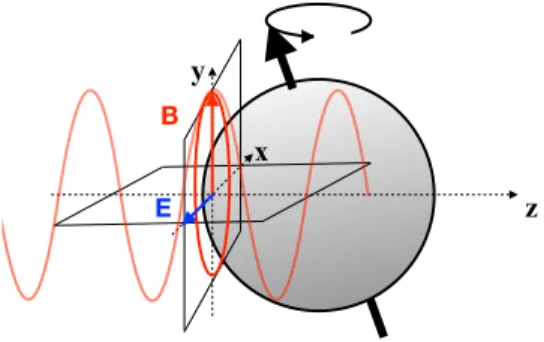
Polarizabilities describe how the components of an object collectively react to external elec-tromagnetic fields. In particular, spin-polarizabilities quantify the object’s spin precession un-der an electromagnetic field, see Fig. 1. The spin-polarizabilities, initially defined with real photons, can be generalized to virtual photons such as those used to probe the neutron in our experiment (see Fig. 2). The energy-momentum transferred between the electron and
neu-z B
E
x y
FIG. 1: Spin-polarizabilities quantify the precession (curled black arrow) of the spin of the neutron (black arrow and gray sphere, respectively) under electromagnetic fields (electric fieldE: blue arrow; magnetic fieldB: red arrow). Electromagnetic waves formed by real photons have E and B and polar-ization vectors perpendicular to the wave propagation directionz. Generalized spin-polarizabilties arise with virtual photons which also have a longitudinal polarization component.
Virtual photon Incident Electron Scattered Electron Target neutron Neutron debris
FIG. 2: Electron scattering off a neutron by the one-photon exchange process. If both the inci-dent electron and the neutron are polarized, this process can be used to measure the generalized spin-polarizabilities of the neutron.
tron is (⌫, q), with Q2 = q2 ⌫2 characterizing the space-time scale at which we probe the neutron. While real photons (Q2 = 0) only have transverse polarizations, mediating virtual photons (Q2 6= 0) are transversely (T) or longitudinally (L) polarized. Thus, two contributions to the spin-polarizability arise, one from the transverse-transverse (TT) interference called the forward spin-polarizability 0(Q2), and the other from the longitudinal-transverse (LT)
interfer-ence, called the Longitudinal-Transverse interference polarizability LT(Q2)and available only with virtual photons. The additional polarization direction L and the ensuing interference term offer extra latitude to test theories describing the Strong Interaction.
The theoretical basis to measure LT(Q2)originates from a work of Gell-Mann, Goldberger and Thirring [7,8]. This work lead relations between the cross-sections measured in polarized electron-nucleon scattering (Fig.2) and the spin-polarizabilities:
0(Q2) = 1 2⇡2 Z 1 ⌫0 ⌫2 TT(⌫, Q2) ⌫2 d⌫, (1) LT(Q2) = ✓ 1 2⇡2 ◆ Z 1 ⌫0 ⌫Q LT(⌫, Q2) ⌫2 d⌫, (2)
where TT and LT are respectively the TT and LT interference cross-section, = ⌫
Q2
/2M[9] is the photon flux factor with ⌫ the energy transfer and ⌫0the photoproduction
thresh-old. The ⌫ 2weighting factor facilitates the convergence of the integral and minimizes the issue that ⌫ ! 1 cannot be reached experimentally.
An outstanding feature of LT(Q2)at low Q2 is that the (1232) is not expected to signif-icantly contribute to the LT-interference cross section, since exciting the (1232) overwhelm-ingly involves transverse photons. This should alleviate the difficulty of including the (1232) in EFT calculations, making them more robust. However, the first measurement of LT(Q2) from JLab experiment E94-010 [12] done at Q2 0.1GeV2strongly disagreed with EFT cal-culations [10, 11]. This surprising result, known as the “ LT puzzle” [13], triggered improved EFT calculations [14] which now explicitly include the (1232) [2–4], and measurements of LTat lower Q2where EFT can be best tested. New data of LTon the neutron at very low Q2, taken during experiment JLab E97-110, are presented next.
Eq. (2) allows measuring n
LT(Q2)(the superscript n indicates neutron quantities) by scat-tering polarized electrons off polarized neutrons in 3He nuclei. The measured cross-section
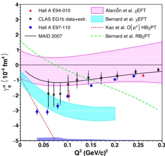
2 (GeV/c) 2 Q 0 0.05 0.1 0.15 0.2 0.25 0.3 4 fm -4 10 LT n δ 2 − 1 − 0 1 2 3 MAID 2007 Hall A E94-010 Hall A E97-110 EFT χ Alarcon et al. EFT χ Bernard et al. PT χ HB 4 p Kao et al. O PT χ Bernard et al. RB ' FIG. 3: n
LT(Q2) from experiment E97-110, compared to earlier E94-010 data [12], EFT calcula-tions [2,4,10,11] and the MAID model [15]. The inner error bars, sometimes too small to be visible, represent the statistical uncertainties. The outer error bars show the combined statistical and uncorrelated systematic uncertainties. The correlated systematic uncertainty is indicated by the band at the bottom.
LT(⌫, Q2) is used with Eq. (2) to form n
LT(Q2), after which nuclear corrections are applied (see supplemental material). Our data are shown in Fig.3. They agree with earlier data from E94-010 at larger Q2 [12] while reaching much lower Q2 where the EFT is expected to work well. The measurement can be compared to EFT calculations [2,4, 10, 11] and a model pa-rameterization of the world photo- and electro-production data called MAID [15]. Earlier EFT calculations [10, 11] used different approaches (Heavy Baryon and Relativistic Baryon chiral perturbation theory: HB PT and RB PT, respectively), and furthermore either neglected the (1232)degrees of freedom, or included it approximately. Newer calculations [2–4] account for the (1232) explicitly by using a perturbative expansion, but they differ in their choice of expansion parameter. Despite this theoretical improvement and the small Q2 reach that places our data well in the validity domain of EFT, our n
2 (GeV/c) 2 Q 0 0.05 0.1 0.15 0.2 0.25 0.3 4 fm -4 10 n 0 γ 5 − 4 − 3 − 2 − 1 − 0 1 2 3 4 Hall A E94-010 CLAS EG1b data+extr. Hall A E97-110 MAID 2007 EFT χ Alarcon et al. EFT χ Bernard et al. PT χ HB 4 p Kao et al. O PT χ Bernard et al. RB '
FIG. 4: Same as Fig.3but for the other generalized spin-polarizability, n 0(Q2). This is even more surprising because the latest EFT calculations of n
LTagree with each other, suggesting that calculations for this particular observable should be under control. However, our data reveal an opposite trend with Q2 to that of all the EFT calculations.
This startling discrepancy demanded further scrutinization of our data. They are compatible with the E94-010 data where they overlap. This is also true for n
0(Q2), which we measured concurrently and show in Fig.4. The measured n
0(Q2)also agrees with data from CLAS ex-periment EG1 [16], which used a target and detectors that are very different from E97-110 and E94-010. Our n
0(Q2)data generally disagree with EFT calculations. Since 0(Q2)does not benefit from the suppression of the (1232) contribution, and since n
0(Q2) predictions do not reach a consensus, this disagreement is not entirely surprising, in contrast to the unex-pected n
LT(Q2) disagreement. Interestingly, we can also study with our data the Schwinger relation [17], which has a similar definition but without ⌫ 2 weighting in its integrand. The Schwinger integral is shown in Fig.5of the Supplemental Materials and displays a similar Q2 -behavior as LT, irrespective of the different ⌫-weighting. Other integrals without ⌫ 2weighting
formed using our data and reported in [18] did not display the surprisingly strong disagreements with the predictions seen here.
In conclusion, we measured the spin-polarizability n
LT(Q2) well into the domain where EFT is expected to describe reliably the nucleon properties. Surprisingly, data and predic-tions disagree significantly. This is perplexing since LTwas expected to be a robust prediction of EFT and the earlier finding that the (1232) is important for the calculation of LT had been addressed. Our data indicate that both the TT and LT interferences of the electromagnetic field’s components induce a clear spin precession of the neutron. While it was predicted by all calculations and models that the LT term influence should intensify at small Q2, our data reveal the opposite trend. Lattice QCD calculations of LT(Q2) are possible [19], but not yet avail-able. Our data motivate such calculations since the measured generalized spin-polarizabilities underline a current lack of reliable quantitative descriptions of the Strong Interaction at the nucleon-size scale, even for “gold-plated” observables such as LT.
Method Summary The data were acquired in the Hall A [21] of Jefferson Lab (JLab) dur-ing experiment E97-110 [18]. The probing virtual photons were produced by a longitudinally polarized electron beam during its scattering off a polarized3He target [21]. The beam polar-ization, flipped pseudo-randomly at 30 Hz and monitored by Møller and Compton polarimeters, was 75.0 ± 2.3%. The beam energies ranged from 1.1 to 4.4 GeV and the beam current was typically a few µA. Since free neutrons are unstable we used3He nuclei as an effective polar-ized neutron target. To first-order, polarpolar-ized3He nuclei are equivalent to polarized neutrons because the3He’s nucleons (two protons and one neutron) are mostly in an S-state, so the Pauli exclusion principle dictates that in the S-state, the proton spins point oppositely, yielding no net contribution to the3He spin. The gaseous (⇡ 12 atm)3He was contained in a 40 cm-long glass cylinder, and polarized by spin-exchange optical pumping of Rubidium atoms. Helmholtz coils provided a parallel or transverse 2.5 mT field used to maintain the polarization, to orient
it longitudinally or perpendicularly (in-plane) to the beam direction, and to aid in performing polarimetry. The average target polarization in-beam was (39.0 ± 1.6)%. The scattered elec-trons from the reaction ~3He(~e, e0) were detected by a High Resolution Spectrometer (HRS) [21] supplemented by a dipole magnet [22] allowing scattering angles down to 6 . Behind the HRS, drift chambers provided particle tracking, scintillator planes enabled the data acquisition trig-ger, and a gas Cherenkov counter and electromagnetic calorimeters ensured the identification of the particle type. Both spin asymmetries and absolute cross-sections were measured and used to form TT(⌫, Q2) and LT(⌫, Q2) [6]. They were integrated according to Eqs. (1) and (2) to obtain the integrals n
0(Q2)and nLT(Q2). The unmeasured part of the integral at large ⌫ is negligible for n
0 and LTn due to the ⌫-weighting of their integrands. The values 0n(Q2) and n
LT(Q2)with their uncertainties are provided in the Supplemental Material, as well as the inte-gration range which was covered. While polarized3He nuclei are effectively polarized neutrons to good approximation, nuclear corrections are needed to obtain genuine neutron information. The prescription of Ref. [23] was used for the correction. Typically, the correction increases by 20% the absolute values of the generalized spin-polarizabilities except for the lowest Q2 point for n
LTwhere the correction is smaller, less than 7%. The relative uncertainty on this correction is estimated to be 6 to 14%, the higher uncertainties corresponding to our lowest Q2values. The other main systematic uncertainties come from the absolute cross-sections (3.5 to 4.5%), target and beam polarizations (3 to 5% and 3.5%, respectively), and radiative corrections (3 to 7%). Data availability Experimental data that support the findings of this study are provided in the supplemental material or are available from J.P Chen, A. Deur, C. Peng or V. Sulkosky upon request.
Code availability The computer codes that support the plots within this paper and the findings of this study are available from J.P Chen, A. Deur, C. Peng or V. Sulkosky upon request.
Author contributions The members of the Jefferson Lab E97-110 Collaboration constructed and operated the experimental equipment used in this experiment. All authors contributed to the data collection, experiment design and commissioning, data processing, data analysis or Monte Carlo simulations. The following authors especially contributed to the main data analysis: J.P Chen, C. Peng, A. Deur, and V. Sulkosky.
Acknowledgments
We acknowledge the outstanding support of the Jefferson Lab Hall A technical staff and the Physics and Accelerator Divisions that made this work possible. We thank A. Deltuva, J. Golak, F. Hagelstein, H. Krebs, V. Lensky, U.-G. Meißner, V. Pascalutsa, G. Salm`e, S. Scopetta and M. Vanderhaeghen for useful discussions and for sharing their calculations. We are grateful to V. Pascalutsa and M. Vanderhaeghen for suggesting to compare the data to the Schwinger relation. This material is based upon work supported by the U.S. Department of Energy, Office of Science, Office of Nuclear Physics under contract DE-AC05-06OR23177, and by the NSF under grant PHY-0099557.
[1] V. Bernard, N. Kaiser and U. G. Meissner,Int. J. Mod. Phys. E4, 193 (1995)
[2] V. Bernard, E. Epelbaum, H. Krebs and U. G. Meissner,Phys. Rev. D87, no. 5, 054032 (2013) [3] V. Lensky, J. M. Alarc´on and V. Pascalutsa,Phys. Rev. C90, no. 5, 055202 (2014)
[4] J. M. Alarc´on, F. Hagelstein, V. Lensky and V. Pascalutsa,arXiv:2006.08626 [5] A. Deur, S. J. Brodsky and G. F. de Teramond,Prog. Part. Nucl. Phys.90, 1 (2016) [6] A. Deur, S. J. Brodsky and G. F. De T´eramond,Rep. Prog. Phys.,82, 7 (2019) [7] M. Gell-Mann, M. L. Goldberger and W. E. Thirring,Phys. Rev.95, 1612 (1954) [8] P. A. M. Guichon, G. Q. Liu and A. W. Thomas,Nucl. Phys. A591, 606 (1995) [9] L. N. Hand,Phys. Rev.129, 1834 (1963)
[10] V. Bernard, T. R. Hemmert and U. G. Meissner,Phys. Rev. D67, 076008 (2003) [11] C. W. Kao, T. Spitzenberg and M. Vanderhaeghen,Phys. Rev. D67, 016001 (2003) [12] M. Amarian et al., [E94-010 experiment]Phys. Rev. Lett.93, 152301 (2004) [13] J. P. Chen,Int. J. Mod. Phys. E19, 1893 (2010)
[14] F. Hagelstein, R. Miskimen and V. Pascalutsa,Prog. Part. Nucl. Phys.88, 29-97 (2016) [15] D. Drechsel, O. Hanstein, S. S. Kamalov and L. Tiator,Nucl. Phys. A645, 145 (1999) [16] N. Guler et al., [EG1b experiment]Phys. Rev. C92, no. 5, 055201 (2015)
[17] J. S. Schwinger,Proc. Nat. Acad. Sci.72, 1 (1975)
[18] V. Sulkosky et al. [E97-110 Collaboration],Phys. Lett. B805, 135428 (2020) [19] A. J. Chambers et al.,Phys. Rev. Lett.118, 24 242001 (2017)
[20] H. Burkhardt and W. N. Cottingham,Annals Phys.56, 453 (1970) [21] J. Alcorn et al.,Nucl. Instrum. Meth. A522, 294 (2004)
[22] F. Garibaldi et al.Phys. Rev. C99, 054309 (2019)
[23] C. Ciofi degli Atti and S. Scopetta,Phys. Lett. B404, 223 (1997)
[24] K. P. Adhikari et al., [EG4 experiment]Phys. Rev. Lett.120, 062501 (2018) [25] S. D. Bass, M. Skurzok and P. Moskal,Phys. Rev. C98, 025209 (2018) [26] Z. Ye, J. Arrington, R. J. Hill and G. Lee,Phys. Lett. B777, 8-15 (2018) [27] K. Helbing,Prog. Part. Nucl. Phys.57, 405-469 (2006)
[28] S. B. Gerasimov, Sov. J. Nucl. Phys.2, 430 (1966)
Supplemental material
Verification of the data quality using the Schwinger relation: A relation similar to that of LT but without ⌫ 2weighting is:
ILT(Q2) ⌘ ✓ M2 ↵⇡2 ◆ Z 1 ⌫0 h LT(⌫, Q 2) Q⌫ i Q=0d⌫ (3)
Schwinger predicted that ILT(Q2) !
Q2!0 et [17], with the summer anomalous magnetic
moment of the target particle and et its electric charge. This prediction is general, e.g. it does not use EFT. ILT(Q2)having no ⌫-weighting, the large ⌫ contribution to the integral is not negligible. Since this contribution to the integral cannot be measured, a parameterization based on the model described in [24] completed by a Regge-based parameterization [25] for the largest ⌫ part was used to extrapolate it. Our measurement of In
LT(Q2)is shown in Fig.5. Our measurement of In
LT(Q2) without the Regge-based parameterization [25] for the large-⌫ part (open symbols), which is suppressed in LT(Q2), displays a similar pattern as n
LT(Q2). The Gerasimov-Drell-Hearn (GDH) relation [28,29] can be used to extrapolate our In
LT(Q2)to Q2 = 0and provided that the GDH relation is correct, which is widely expected and supported by dedicated experimental studies [27], our data satisfy Schwinger’s prediction that In
LT(0) = 0[17]. Our trend contrasts with the MAID model and presumably the EFT calculations, since MAID tracks those (see Fig.3). This suggests that the problem lies in the theoretical description of the neutron structure.
Integrands: The integrands (excluding the ⌫-weighting) of n
LT(Q2), ILTn (Q2) and 0n, are displayed in Figs.6and 7.
2 (GeV/c) 2 Q 0 0.1 0.2 0.3 2 Q LT n I 2 − 1 − 0 1 2 E97-110 Resonance MAID 2007 E97-110 Total + FF Param. 1 Γ GDH Schwinger Relation FIG. 5: The In
LT(Q2) integral. The open symbols are our results without the large ⌫ part of ILT. The filled blue circles are our results for the full ILT, using an estimate for the large ⌫ contribution. The inner error bars represent the statistical uncertainties. The outer error bars show the combined statistical and uncorrelated systematic uncertainties. The correlated systematic uncertainty is indicated by the band. The Schwinger relation [17] for the neutron predicts In
LT(0) = 0at Q2 = 0. The plain line shows the MAID model [15] (resonance only, to be compared to the open symbols). The dashed line uses the GDH [28,29] and Burkhardt-Cottingham [20] relations, together with an elastic form factor parameterization [26], to obtain In
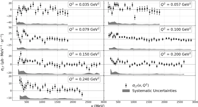
FIG. 6: The longitudinal-transverse interference cross-section LT(⌫, Q2)for3He at the Q2 values at which it is integrated into LT(Q2)(Eq.2) or ILT(Q2)(Eq.3). The nuclear corrections [23] necessary to obtain the neutron information from the3He data are applied after the integration. The prominent (1232)contribution seen for TT(⌫, Q2)in Fig.7is not present here, in agreement with the expectation that the role of (1232) is suppressed in LT-interference quantities.
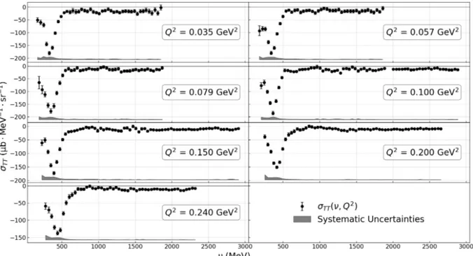
FIG. 7: The transverse-transverse cross-section TT(⌫, Q2)for3He at the Q2values at which it is inte-grated to form 0(Eq.1). The nuclear corrections providing the neutron information from the3He data are applied after the integration. The prominent negative peak at small-⌫ is the (1232) contribution.
Data table
Q2 x
min(Wmax) 0n(Q2)±(stat)±(syst) LTn (Q2)±(stat)±(syst) ILT(Q2)n±(stat)±(syst) ILTmeas. ILT 0.035 0.0112 (2.00) 3.094± 0.129 ± 0.270 0.383± 0.326 ± 0.677 1.112± 0.316 ± 0.606 0.26 0.057 0.0181 (2.00) 3.117± 0.141 ± 0.259 0.225 ± 0.071 ± 0.197 0.862± 0.136±0.389 -0.48 0.079 0.0249 (2.00) 2.717± 0.140 ± 0.270 0.435 ± 0.098 ± 0.195 0.721± 0.149 ± 0.314 -1.09 0.100 0.0183 (2.50) 2.070± 0.074 ± 0.170 0.491 ± 0.083 ± 0.209 0.126± 0.114 ± 0.329 -8.65 0.150 0.0273 (2.50) 1.370± 0.051 ± 0.125 0.215 ± 0.052 ± 0.173 0.266± 0.057 ± 0.233 -1.72 0.200 0.0398 (2.40) 0.965± 0.032 ± 0.065 0.111 ± 0.028 ± 0.091 0.345± 0.055 ± 0.267 -1.13 0.240 0.0547 (2.25) 0.742± 0.026 ± 0.050 0.108 ± 0.020 ± 0.043 0.267± 0.067 ± 0.192 -1.91
TABLE I: Data and kinematics. From left to right: Four-momentum transfer ([GeV]2); mimimum x ⌘ Q2/
2m⌫ value experimentally covered (equivalent maximum invariant W [GeV] (W = (M2 + 2M ⌫ Q2)1/2; n
0(Q2)± statistical uncertainty ± systematic uncertainty; nLT(Q2)± statistical uncertainty ± systematic uncertainty; ILT(Q2)n, including an estimate for the unmeasured contribution below xmin, ± statistical uncertainty ± systematic uncertainty; Ratio of measured to total ILT(Q2)n. The unmeasured parts of n
![FIG. 3: LT n (Q 2 ) from experiment E97-110, compared to earlier E94-010 data [12], EFT calcula- calcula-tions [2, 4, 10, 11] and the MAID model [15]](https://thumb-eu.123doks.com/thumbv2/123doknet/13972446.453790/7.918.288.625.157.479/experiment-compared-earlier-calcula-calcula-tions-maid-model.webp)