Bayesian networks for cardiovascular monitoring

Bayesian Networks for Cardiovascular Monitoring

by

Jennifer Roberts

B. S., Electrical Engineering

NOV

2 2006

B. S., Computer Science

University of Maryland, College Park (2004)

Submitted to the Department of Electrical Engineering

and Computer Science

_BARKER

in partial fulfillment of the requirements for the degree of

Master of Science in Electrical Engineering

at the

MASSACHUSETTS INSTITUTE OF TECHNOLOGY

May

2006-©

Jennifer Roberts, 9MMVI. All rights reserved.

The author hereby grants to MIT permission to reproduce and

distribute publicly paper and electronic copies of this thesis document

in whole or in part.

A uthor ...

.

.

.

..

.

.

.

.

Department of Electrical Engineering

and Computer Science

May 12, 2006

Certified by

...

...

George Verghese

Professor

Thesis Supervisor

C ertified by ...

...

Thomas Heldt

j

ostdctoral Research Associate

gesis Supervisor

A ccepted by ....

...

Arthur C. Smith

Chairman, Department Committee on Graduate Students

Bayesian Networks for Cardiovascular Monitoring

by

Jennifer Roberts

Submitted to the Department of Electrical Engineering and Computer Science

on May 12, 2006, in partial fulfillment of the requirements for the degree of

Master of Science in Electrical Engineering

Abstract

In the Intensive Care Unit, physicians have access to many types of information when treating patients. Physicians attempt to consider as much of the relevant information as possible, but the astronomically large amounts of data collected make it impossible to consider all available information within a reasonable amount of time. In this thesis,

I explore Bayesian Networks as a way to integrate patient data into a probabilistic

model. I present a small Bayesian Network model of the cardiovascular system and analyze the network's ability to estimate unknown patient parameters using available patient information. I test the network's estimation capabilities using both simulated and real patient data, and I discuss ways to exploit the network's ability to adapt to patient data and learn relationships between patient variables.

Thesis Supervisor: George Verghese Title: Professor of Electrical Engineering Thesis Supervisor: Thomas Heldt

Acknowledgments

I would like to thank Dr. Thomas Heldt for his support, encouragement, and

guid-ance. He has been a wonderful mentor, and his continual feedback has helped me throughout my time at MIT. I also thank Professor George Verghese for his gentle support and thoughtful guidance. I appreciate the way he always looks out for his stu-dents. I thank Tushar Parlikar for supplying me with simulated and real patient data and for contributing a section to the thesis. Without his help, this work would not have been possible. I also thank my parents, Tom and Valerie; my sister, Becca; my grandmother, Dolores; and my boyfriend, Chen, for their continued love and support.

I graciously thank the Fannie and John Hertz Foundation and the National Science

Foundation for their financial support. This work is made possible by grant ROl

EB001659 from the National Institute of Biomedical Imaging and Bioengineering of

Contents

1 Introduction 13

1.1 Using Models to Integrate Patient Data . . . . 13

1.2 Traditional Cardiovascular Models . . . . 15

1.3 Bayesian Networks in Medicine . . . . 16

1.4 G oals . . . . 18

1.5 O utline . . . . 18

2 Bayesian Networks 21 2.1 What is a Bayesian Network? . . . . 21

2.2 Important Terminology . . . . 25

2.3 A Bayesian Network Model of the Cardiovascular System . . . . 27

3 Learning Algorithms 31 3.1 Modeling the Bayesian Network Parameters using Dirichlet Distributions 31 3.1.1 Introduction to Dirichlet Distributions . . . . 32

3.1.2 Modeling Nodes with Multiple Parents . . . . 35

3.1.3 Model Complexity . . . . 36

3.2 Setting and Updating the Dirichlet Distributions . . . . 37

3.3 Learning Algorithms . . . . 41

3.3.1 Batch Learning . . . . 41

3.3.2 Sequential Learning with Transient Memory . . . . 42

4 Application to Patient Data

4.1 The Bayesian Network ...

4.2 Preliminary Tests using Simulated Data . . . . 4.2.1 Simulated Data . . . . 4.2.2 Network Training . . . . 4.2.3 Testing the Trained Network . . . . 4.2.4 Error Analysis . . . . 4.2.5 R esults . . . . 4.3 Tests using Real Patient Data . . . . 4.3.1 Patient Data . . . . 4.3.2 Batch Training and Prediction . . . . 4.3.3 Single Beat Prediction using Sequential Training . . 4.3.4 Multiple Beat Prediction using Sequential Training 4.3.5 Combinational Learning . . . .

5 Discussion and Future Work

5.1 D iscussion . . . .

5.2 Future Work . . . .

5.2.1 Further Analysis of the Current Network

5.2.2 Real Patient Data . . . .

5.2.3 Expansion of the Current Model . . . . .

5.3 Conclusion . . . .

. . . . . . . .

Model and Algorithms

. . . . . . . . . . . . A Alternate Bayesian Network Model which Incorporates Treatment

Information 77

B Simulation Parameters and Bayesian Network Quantization Values 81 45 45 47 47 51 51 52 52 53 54 56 57 64 67 69 69 70 70 74 75 76

List of Figures

2-1 A directed acyclic graph. . . . . 22 2-2 A Bayesian Network example, where HR denotes heart rate, CO

de-notes cardiac output, and NVI dede-notes net volume inflow. . . . . 24 2-3 A simple Bayesian Network model of the cardiovascular system. . . 27

3-1 A simple Bayesian Network model of the cardiovascular system. . . 32 3-2 A Bayesian Network example that does not exhibit an equivalent

sam-ple size. . . . . 39 3-3 Examples of two-parameter Dirichlet distributions, otherwise known

as beta distributions. . . . . 40

4-1 A simple Bayesian Network model of the cardiovascular system. . . . 46

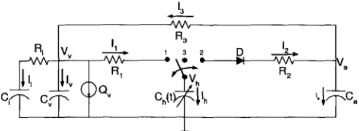
4-2 The simple pulsatile cardiovascular model. The model has a single ventricular compartment (R1, Ch(t), R2), an arterial compartment (Ca,

R3), _{a venous compartment (C,), an interstitial fluid compartment (Ci,}

Ri), and a blood infusion or hemorrhage source

Q..

4-3 Simulated data . . . . 50

4-4 Conditional probability mass functions for BP, given CO and TPR. Each plot shows the conditional PMF of BP for a particular set of CO and TPR values. . . . . 53

4-5 Data samples containing thermodilution measurements. The stars in-dicate actual values while the crosses represent quantized values. The data samples are plotted versus the sample set numbers. . . . . 54

4-6 Data from patient 11007. Original waveforms are shown in blue, quan-tized waveforms are shown in green, and the quantization thresholds

are shown in aqua. . . . . 55

4-7 Comparison of actual Patient 11007 TPR, CO, and SV waveforms to estimated waveforms obtained using a network solely trained on the Gold Standard Data. . . . . 57

4-8 Estimates when the Bayesian Network is sequentially trained with var-ious finite memory sizes and tested on the Patient 11007 data. In a,

b, c, and d, the memory sizes are 100, 1000, 5000, and 8000 beats,

respectively. . . . . 61

4-9 Comparison of the actual non-median filtered Patient 6696 waveforms with the MMSE estimated waveforms obtained by first sequentially training the Bayesian Network on the Gold Standard Data and then sequentially training and testing the network on Patient 6696 data with a history size of 1000 data points. . . . . 63

4-10 1661-beat MMSE and naive estimates obtained when the network is trained using a sequential memory size of 5000 beats. The bottom two plots show the HR and BP evidence presented to the network during training and inference. . . . . 66

4-11 1661-beat MMSE and naive estimates obtained when the network is first batch trained on the Gold Standard Data and then sequentially trained on the Patient 11007 data using a finite memory size of 5000 beats. The bottom two plots show the HR and BP evidence presented to the network during training and inference. . . . . 68

A-1 A simple model of the cardiovascular system . . . . 78

A-2 Patient data used to initialize the network parameters . . . . 78

A-3 Conditional PMF from a trained network: Conditional PMF of BP

given TPR and CO . . . . 79

List of Tables

4.1 Description of the training data segments. . . . . 49

4.2 A comparison of the mean error rates and standard deviations for the

data sets with 250 second segments, where MMSE denotes the mini-mum mean square error estimates and MAP denotes the MAP estimates. 52 4.3 Absolute error rates for the MMSE estimates when the network is

sequentially trained on Patient 11007 data using finite memory sizes of 100, 1000, 5000, and 8000 beats. ... 62

4.4 Average percent of the time that the Bayesian Network estimates were more accurate than the naive estimates for CO and SV. . . . . 65

B.1 Nominal parameters used to create the simulated data. . . . . 81

B.2 Bin numbers and corresponding quantization values used when training the Bayesian Network on simulated patient data. . . . . 82

B.3 Bin numbers and corresponding quantization values used when training the Bayesian Network on real patient data. . . . . 82

Chapter 1

Introduction

Bayesian Networks provide a flexible way of incorporating different types of infor-mation into a single probabilistic model. In a medical setting, one can use these networks to create a patient model that incorporates lab test results, clinician ob-servations, vital signs, and other forms of qualitative and quantitative patient data. This thesis will outline a mathematical framework for incorporating Bayesian Net-works into cardiovascular models for the Intensive Care Unit and explore effective ways to assimilate new patient information into the Bayesian models.

1.1

Using Models to Integrate Patient Data

Physicians have access to many types of information when treating patients. For example, they can examine real-time waveform data like blood pressures and electro-cardiogram (ECG) recordings; data trends like time-averaged heart rate; intermittent measurements like body temperature and lab results; and qualitative observations like reported dizziness and nausea.

Within the Intensive Care Unit (ICU), physicians attempt to consider as much of the relevant information as possible, but the astronomically large amounts of data collected make it impossible to consider all available information within a reason-able amount of time. In addition, not all of the data collected is helpful in its raw form, but sufficient statistics taken from such data might help physicians gain a more

thorough understanding of recent changes in the patient's state. Because of this, we are exploring ways to integrate different types of patient data into more synthesized forms (see http://mimic.mit.edu/).

Models provide one way of synthesizing multiple observations of the same com-plex system, and Bayesian Networks provide a probabilistic framework for developing patient models. With Bayesian Networks, we can incorporate different data types into a single model and use Bayesian inference to probabilistically estimate variables of interest, even when data is missing.

By using models to synthesize data, we hope to improve monitoring capabilities

and move patient monitoring in new directions by generating more accurate alarms, making predictive diagnoses, providing clinical hypotheses, predicting treatment out-comes, and helping doctors make more informed clinical decisions. As an example, alarms generated by current monitoring systems have extremely high false alarm rates, and because they go off so frequently, nurses learn to ignore them. Often these alarms are generated by observing only a single patient variable at a time. By syn-thesizing more of the available patient data, systems could generate more accurate alarms that would convey more reliable information.

Similarly, current monitoring systems measure and display patient vital signs, but they only perform a limited amount of analysis on the measured waveforms. By using models to synthesize patient data, monitoring systems might one day perform analyses that could diagnose problems before they become critical, perhaps predicting a patient's impending hemodynamic crisis minutes in advance so that doctors can perform preventive treatments instead of reactive ones. Advanced systems might further use patient models to simulate treatment options and use the simulation results to guide doctors toward more effective treatments. Systems might also learn to identify the true source of a medical problem so that doctors could address problem sources instead of treating symptoms. This discussion touches on just a few of the ways that a more synthesized approach might aid both clinicians and patients.

1.2

Traditional Cardiovascular Models

As mentioned before, models provide one way of synthesizing different observations of the same complex system. Many traditional cardiovascular models are derived from physiology by using computational models of the heart and blood vessels. Such computational models provide a set of differential equations that can be mapped to an equivalent set of circuit equations. Within the equivalent circuit models, volt-age represents pressure, current represents blood flow, resistance represents blood vessel resistance, and capacitance represents compliance, a measure of vascular dis-tensibility. These circuit models are used to simulate cardiovascular dynamics and gain a thorough understanding of how components within the cardiovascular system interact.

A number of cardiovascular circuit models exist with varying levels of complexity.

The Windkessel model, for example, describes the arterial portion of the circulatory system with only two parameters. In contrast, other models like those described in [4, 6, 14] contain many vascular compartments representing the right and left ventricles, the systemic veins and arteries, the pulmonary veins and arteries, and sometimes even other organs in the body. Some models simulate pulsatile behavior [2, 4], while others track trend behavior [12]. Timothy Davis's thesis contains a short survey of several of the early lumped-parameter hemodynamic models including

CVSIM, CVSAD, and the Windkessel model [3].

While these physiological models are complex enough to track real patient data, using these models to do so in real time is extremely challenging. Within the ICU, only a limited number of patient vital signs are consistently available. These signals do not provide enough information to accurately estimate more than a small number of model parameters [14]. This means that many parameters in the larger physiological models cannot be estimated accurately using commonly available patient data. In addition, real data is often extremely noisy. Signals frequently disappear or become overwhelmed by artifacts when patients move or become excited. These artifacts make it even more difficult to robustly track patient trends using physiological models.

In addition, conventional physiological models do not use all available informa-tion when attempting to track patient state. They do not incorporate qualitative observations like "the patient is dizzy" or "the patient is bleeding heavily." They also fail to incorporate information about the patient's diagnosis. Similarly, physiological models fail to assimilate intermittent data like that obtained through lab reports, nurses notes, and medication charts, into their calculations. These types of informa-tion convey important informainforma-tion about the patient's state and should be taken into account.

In order to integrate both qualitative and quantitative information into modeling efforts, we use Bayesian Network models to complement the traditional physiologi-cal ones. With Bayesian Networks, we can incorporate non-numeric, discrete, and continuous information into the same model. Bayesian Networks can robustly use intermittent data when it is available and function reliably when such data is not available. These networks provide a stochastic framework for estimating physiological model parameters, a framework we can rely on when patient measurements become noisy or unreliable.

1.3

Bayesian Networks in Medicine

Within the medical field, Bayesian networks have frequently been used for diagnosis

[8, 16, 11, 10], patient monitoring [1], and therapy planning [13]. For instance, the

Heart Disease Program [8] uses a several-hundred-node Bayesian Network to create a list of most probable cardiovascular diagnoses, given patient symptoms. While accurate, the network is difficult to maintain because of the large number of network parameters set by expert opinion.

VentPlan [13], a ventilator therapy planner, attempted to use a Bayesian Network to incorporate qualitative data into a mathematical model of the pulmonary system.

By exploiting the Bayesian Network, the program used qualitative patient information

to initialize parameters of the mathematical model. The mathematical model then ran simulations to determine the best ventilator treatment plan, given the current

patient state. Overall, the system proposed treatment plans that changed ventilator settings in the correct direction, but experts disagreed about the proper magnitude of change needed.

Using Bayesian Networks, Berzuini et al. [1] propose a methodology that uses in-formation about previous patients to monitor current patients. Within this method-ology, each patient is described using the same parameterized model. Each set of patient parameters is assumed to be drawn from the same unknown probability dis-tribution. The current patient receives an additional parameter that rates how typical his or her response is in comparison with the general population. If the current pa-tient's response seems typical, information about previous patient parameters is used to set the current patient's parameters. Otherwise, current patient parameters are set using only information about the current patient. The relative weight assigned to information from previous patients versus information from the current patient changes based on the current patient's typicality. With a Bayesian Network, Berzuini et al. explicitly described how current patient parameters depend information about both current and previous patients. They then used this methodology to model how patients' white blood counts respond to chemotherapy. By conditioning on informa-tion obtained from previous patients, these researchers more accurately tracked white blood count for patients deemed typical of the general population.

Recently, much work has been done on sequentially learning Bayesian Network structures from data [5]. Algorithms that perform this type of learning are often used in biological contexts to identify large biological networks, but have also been used in other contexts to learn models directly from data. The book by Neapolitan contains a summary of some of these applications and research within the field of Learning Bayesian Networks [10].

In this thesis, I focus on developing relatively simple Bayesian Network models of the cardiovascular system that capture necessary patient dynamics without adding extraneous model parameters that are difficult to estimate. Unlike the Heart Dis-ease Program, I explore much simpler models whose parameters can be learned and updated based on available patient data. The current goal is not to diagnose every

type of cardiovascular disease, but instead to estimate unavailable information about a patient's state based on data generally available in the ICU. We aim to develop a Bayesian model for the cardiovascular system similar to the Bayesian model used

by VentPlan, while exploring ways to balance population data with current patient

history, as in [1].

1.4

Goals

In this thesis, I will describe a methodology for using Bayesian Networks for cardio-vascular monitoring in the Intensive Care Unit. Specifically, I will

" describe a mathematical framework for incorporating Bayesian Network models into cardiovascular patient monitoring systems for the ICU;

" describe a methodology for assimilating new patient information into Bayesian models without disregarding or overemphasizing previously acquired informa-tion;

" describe simulation results that explore whether

- Bayesian Networks can provide good estimates of hidden variables;

- Bayesian Networks can learn and track changes in patient state; " describe future research directions based on simulation results.

1.5

Outline

In Chapter 2, I give an overview of Bayesian Networks and important terminology. Within this chapter, I introduce a simple Bayesian Network model of the cardiovascu-lar system, a model later used to predict unknown patient parameters using available patient data. In Chapter 3, I discuss how to model the network probability distribu-tion parameters, and I describe various ways of using patient data to set and update these parameters. I then apply the Bayesian Network model to both simulated and

real patient data in Chapter 4. In this chapter, I analyze the network's ability to use Bayesian inference to predict unknown patient parameters, given generally avail-able patient information. Chapter 5 concludes with a discussion of the network's capabilities and a discussion of future research directions.

Chapter 2

Bayesian Networks

This chapter provides an overview of Bayesian Networks. It describes how these networks are derived and the types of mathematical issues one needs to consider when creating and implementing a Bayesian Network. In this chapter, I introduce a small Bayesian Network model of the cardiovascular system that I will explore more deeply later in the thesis.

2.1

What is a Bayesian Network?

Before introducing Bayesian Networks, I would like to briefly discuss networks in a more general context. A network, or graph, consists of a set of nodes and a set of edges which connect the nodes. The edges can be either directed or undirected, depending on whether they point from one node to the other or simply indicate a link between nodes.

In a directed graph, like the one shown in Figure 2-1, the edges are represented

by arrows. The triangular end of each arrow is called the head, while the other end is

called the tail. In Figure 2-1, nodes X and W are connected by a directed edge, with node X at the edge's tail and node W at its head. When two nodes are connected by a directed edge, the one at the tail is called the parent, while the one at the head is called the child. Node X, then, has two children, W and Y.

x

w Y

(Z

Figure 2-1: A directed acyclic graph.

node to another. Since arrows can be followed, tail to head, from node X to node

Z, a path exists from X to Z. Since arrows can not be followed in this manner from

node W to node Z, no path exists from W to Z. If a path exists from one node to another, the latter node is called a descendant of the former. Thus, W, Y, and Z are descendants of X, but X, Y, and Z are not descendants of W. Because of this, X, Y, and Z are known as non-descendants of W.

When a path exists from a node back to itself, that path is called a cycle. The graph in Figure 2-1 contains no cycles, but if an arrow was added from Z to X, it would contain a cycle. A directed graph containing no cycles is called a directed acyclic graph.

Networks are used to represent many different types of relationships. In computer networks, the nodes may represent computers while the edges represent wires between the computers. Within a cellular network, nodes represent cell phones or cell towers and directed edges represent down-links or up-links between nodes. In social networks, nodes signify people, while edges signify interactions or relationships between those people.

In a Bayesian Network, nodes represent random variables, and edges represent conditional dependencies between those variables. In this manner, a Bayesian Net-work uses a directed acyclic graph to represent a joint probability distribution. More specifically, a particular graph structure represents a class of probability distribu-tions that factors in a certain way. These factorizadistribu-tions in turn imply a certain set of

conditional independencies. The Markov Property, a property shared by all Bayesian Networks, summarizes the most fundamental set of these implied conditional inde-pendencies. This property states that child nodes are conditionally independent of their non-descendants, given their parents. If a node does not have parents, the node is simply independent of its non-descendants.

Due to the Markov Property, a Bayesian Network's joint probability distribution relates to its graph structure in a straightforward manner. If the network uses N nodes to represent the random variables {xl,.. ., xz}, the joint probability distribution of

{

n

P(Xi,. . .,x,2) =7P(xi the parents of xi).

i=:1

As an example, the class of Markov Chains all factor as n

P(Xi, . . n) = P(xi)- rlP(Xilxi_1),

i=2

and all exhibit the same set of conditional independencies, namely that the past, xi_1, is conditionally independent of the future, xi, given the present, xi. Thus, all

Markov chains with the same number of random variables have a Bayesian network with the same graphical form.

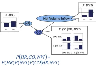
Figure 2-2 displays a simple Bayesian Network, its conditional probability distri-butions, and an equation for its joint probability distribution. Due to the Markov Property, this network structure implies that heart rate (HR) is independent of net

volume inflow (NVI) because heart rate has no parents, and net volume inflow is not

a descendant of heart rate.

The full set of conditional independencies implied by the graph structure can be derived from the set delineated by the Markov Property [10]. When the graph

struc-ture does not imply that a conditional independence exists within a set of nodes,

that set of nodes often exhibits a conditional dependence. Implied conditional de-pendencies of this sort, however, do not exist within every probability distribution

P (OVI)

SP (HR )

PH)(VI CP (CO HR, NVI)

Lo HR

Hijh HR

-LOW NVI H jah NVI

P( HR,CO,NVI )=

P( HR )P( NVI )P(CO|H R,NVI )

Figure 2-2: A Bayesian Network example, where HR denotes heart rate, CO denotes cardiac output, and NVI denotes net volume inflow.

that factors in a manner consistent with the graph structure. To see this, suppose that in Figure 2-2 the top row of the conditional distribution for cardiac output (CO) equaled the bottom row, so CO no longer depended on HR. Then the distribution for

CO would be the same regardless of whether HR was low or high, and the conditional

dependence implied by the arrow from HR to CO would not be present within the underlying probability distribution.

A Bayesian Network is called well-posed if and only if all conditional

dependen-cies implied by the network structure are present in the probability distribution. In other words, a well-posed probability distribution contains only those conditional independencies implied by the network structure and no additional independencies not implied by the structure. When the underlying distribution is not well-posed, it exhibits conditional independencies not reflected in the network structure. In this case, one can always find a different network structure that would better describe the underlying distribution. In the example in the previous paragraph, we could obtain a well-posed network structure by removing the arrow between HR and CO. Unless otherwise specified, all Bayesian Networks discussed in this thesis are well-posed.

given known observations. This involves calculating the a posteriori distribution of the unknown variable, given all available information. The a posteriori distribution can then be used to calculate a best estimate of the unknown variable, given the known data. Because the joint probability distribution is represented as a Bayesian Network, algorithms can efficiently calculate the a posteriori distribution by exploiting the network structure [17, 10].

2.2

Important Terminology

A Bayesian Network model has three interrelated parts: the network structure, the

form of the probability distribution, and the distribution parameters. The network structure, i.e., the directed acyclic graph structure, defines a set of conditional inde-pendencies that the underlying distribution must exhibit, but the form of the distri-bution is otherwise unconstrained. The structure specifies only the manner in which the distribution must factor.

Given a network structure, each node can be assigned a different type of discrete or continuous distribution, conditional on the values of its parents. The form of these conditional node distributions determines the form of the underlying joint probability distribution. For example, if the node variables are jointly Gaussian, the conditional distributions will all be Gaussian.

The distribution form further constrains the underlying distribution defined by the network structure, but one must also set the conditional distribution parameters to have a fully-defined model. These network parameters form the final part of the

Bayesian Network model. In the jointly Gaussian case, the parameter set consists of the conditional means and variances for each network node. Much of the thesis is

devoted to setting and updating these network parameters.

To create a Bayesian Network, one can deduce a probabilistic model from prior experience, learn model structure and distributions from real data, or use some com-bination of these two approaches. In our treatment of Bayesian Networks, we assume that an appropriate network structure and an appropriate probability distribution

form have been derived by experts. This network structure and distribution form remain constant throughout our simulations. We then explore ways of setting and updating the parameters based on prior experience and patient history. Specifically, we are interested in the following issues:

" Parameter Initialization - Initially setting the distribution parameters based on

both expert opinion and general population data by performing some combina-tion of

- Pre-Training Initialization - Setting the distribution parameters based on

previous expectations or expert opinions.

- Batch Learning - Learning distribution parameters from previously

ac-quired patient data sets.

* Inference - Using both the initialized network and available patient information to estimate the values of unknown variables.

" Sequential Parameter Learning - Incrementally updating the distribution

pa-rameters based on new information about the patient.

Many Bayesian Network models are initialized using a set of training data and then employed to make inferences about new data sets, without any type of feedback mechanism to update the probability distributions based on incoming data. In the

ICU setting this type of approach seems flawed, because the model will be trained

on general population data but applied to a particular patient whose characteristics may or may not reflect those of the general population. In order to make the model robust, the network must dynamically adapt to new information obtained from the patient.

Perpetually using the same Bayesian Network model for a given patient also as-sumes that the patient's response is stationary. It asas-sumes we are modeling a station-ary probability distribution. During a hospital stay, however, the patient's response may change based on un-modeled variables. Assuming that the underlying

probabil-Heart Stroke

(:Rate Volume

Total Peripheral Cardiac

Resistance Output

Blood Pressure

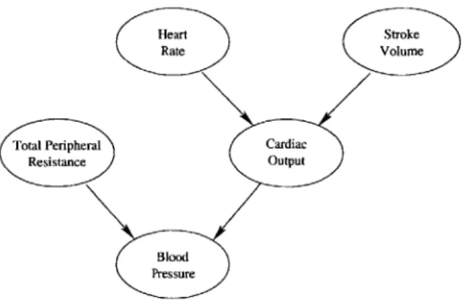
Figure 2-3: A simple Bayesian Network model of the cardiovascular system.

ity distribution is not stationary, we must continually update parameters to capture changes in the underlying probability distribution.

2.3

A Bayesian Network Model of the

Cardiovas-cular System

As mentioned previously, I set out to create a simple Bayesian Network model of the cardiovascular system that captures necessary patient dynamics without adding extraneous model parameters that are difficult to estimate. With the help of medical experts, I developed the Bayesian Network model pictured in Figure 2-3. This model describes a probabilistic relationship among the random variables stroke volume (SV),

mean arterial blood pressure (BP), total peripheral resistance (TPR), cardiac output

(CO), and heart rate (HR) such that

P(SV, BP, TPR, CO, HR)

P(TPR)P(HR)P(SV)P(BPITPR, CO)P(COIHR, SV). (2.1)

The model reflects relationships between cardiac output and the other random vari-ables, namely that CO = HR x SV and CO =- . The network represents a preliminary model upon which one could build in the future.

conditional dependencies and independencies exist between the node variables. Again, these independencies can be derived from the fact that each node is conditionally independent of its non-descendants, given its parents [10]. Assuming well-posedness within Figure 2-3, TPR and CO are conditionally dependent, given BP, and BP is conditionally independent of both HR and SV, given CO. Intuitively, this means that if BP is fixed, knowing the value of TPR yields additional information about CO. Similarly, if CO is fixed, knowing BP yields no additional information about HR or

Sv.

Although the random variables in the Bayesian Network can have probability distributions of an arbitrary form, unless the random variables are Gaussian, in prac-tice continuous distributions are approximated by discrete probability mass functions (PMFs). Within a medical setting, many patient variables are non-Gaussian. For instance, continuous-valued variables like heart rate and blood pressure can only take values within finite-length intervals, so these variables are best modeled by non-Gaussian random variables. Similarly, discrete valued data and non-numeric data realistically take only a finite number of discrete values. Measurement noise may be Gaussian, but the actual patient parameters being measured generally are not.

Within this model, we use a Bayesian Network to model relationships between heart rate, blood pressure, cardiac output, total peripheral resistance, and stroke vol-ume. Realistically, these patient parameters can only take values in a finite range, and median filtering removes much of the Gaussian noise. Because of this, we choose to approximate their continuous probability distributions using discrete probability mass functions. Specifically, we model the random variables in Figure 2-3 using dis-crete probability mass functions that assign probabilities to five quantized random variable values. Each quantized value represents a range of values that a continu-ous version of the same random variables might take. Because of this, the PMFs approximate continuous distributions.

Ultimately, the model depicted in Figure 2-3 could be expanded to incorporate many different types of patient data, but for the research presented in this thesis, this simple model seems appropriate. I previously explored an alternate model which

incorporated treatment information, but due to a lack of acceptable training data (see Appendix A), I chose to focus on the model presented in this section instead. Throughout the remainder of the thesis, I will explore how well this model can capture patient dynamics.

Chapter 3

Learning Algorithms

When creating a Bayesian Network for patient monitoring, one would like a model that relies on both general population information and current patient data. In this chapter, I explain several methodologies for training a Bayesian Network that use both previously available data and data that is gradually presented to the network. These learning algorithms view the Bayesian Network parameters as random variables and update their distributions based on incoming data. I first describe how we model parameters using what are known as Dirichlet distributions and then describe how we exploit these distributions to train the Bayesian Network using patient data. I finally introduce the learning algorithms explored in later chapters.

3.1

Modeling the Bayesian Network Parameters

using Dirichlet Distributions

When a patient visits the hospital, his or her response often changes with time based on un-modeled variables like medications. This means that the probability distribu-tions modeled by the Bayesian Network, and thus the Bayesian Network parameters, also change with time. In a sense, the Bayesian Network parameters become random variables themselves. When performing parameter learning, or training, we in fact view the network parameters as random variables. This allows us to use Bayesian

Heart Stroke

(:Rate Volume

Total Peripheral Cardiac

Resistance Output

Blood Pressure

Figure 3-1: A simple Bayesian Network model of the cardiovascular system. methods to set and update the patient parameters based on patient data.

To treat the Bayesian Network parameters as random variables, we must first define a probabilistic model from them. A good model will reveal how the parameter distributions relate to observed patient training data. This section develops how we model probability mass function (PMF) parameters using Dirichlet distributions. First, we use multinomial distributions to examine how probability parameters relate to observed patient data sets when the probability parameters remain constant. We then expand upon this idea to develop a probabilistic model for the parameters based on relationships between the parameters and observed data sets.

3.1.1

Introduction to Dirichlet Distributions

Before viewing the Bayesian Network parameters as random variables, let us first examine the relationship between a fixed set of patient parameters and multiple sets of observed patient data. Toward this end, let us take a closer look at the HR node of the cardiovascular model reproduced in Figure 3-1. Again, we model HR as a random variable whose values fall into one of five quantization bins. When an observed value falls into bin i, we will say that HR equals i. Thus, HR takes values within the set {1, 2, ... , 5}. Assuming that HR takes the value i with probability

fi,

{fi,

Assume for a moment that we have a training data set which contains N inde-pendent samples of the random variable HR. Let bi be number of times HR takes the

value i during the N independent trials. If we then consider many different training sets containing N independent samples, the number of times HR takes the value i in a particular training set can be viewed as a random variable, Bi. Looking over the many different training sets, the random variables

{B

}

probability mass function of the form:

n! f bi ... ,b 5 if b= N _{and b ;> 0,}

P(B1 = bil ... , B5 = 5b) ={ i bi1

0 otherwise.

This multinomial distribution is a simple extension of a binomial distribution, which describes the probability of observing b1 successes in N independent Bernoulli

tri-als. The multinomial distribution instead describes the probability of observing

{bi,

If we look at a particular data set in which the values {1,... , 5} are observed

{bl,... , b5} times during the N trials, then _N'), the relative frequency with which i is observed, is the maximum likelihood estimate of

fi.

fi

, the probability of value i occurring bi times during N trials is maximized.

During the above analysis, {B1,... , B5}, the number of times that values are ob-served in the training data sets, are seen as random variables. The HR probability parameters, {fi, ... ,

fs},

fi.

and {B1,... , B5} should be fixed, because we generally obtain only a single training

data set with fixed {bi,..., b5}. The probability parameters, on the other hand, are

unknown and may change with time. Thus, these probability parameters are better modeled as random variables themselves.

In order to view the HR probability parameters as random variables, let F be a random variable representing the probability, or 'frequency,' with which HR takes the value i. We then model this set of PMF parameters, {F1,..., F5}, as having what is known as a Dirichlet distribution. The reasons for choosing this

distribu-tion model should become apparent as we describe the Dirichlet distribudistribu-tion and its characteristics.

Using this model, the HR probability parameters {F1,. .., F5} share the following Dirichlet probability density function [10]:

1fF(N) ai-l a2-1 . a.. a -I5

f

p (F1 =

fi,

0 otherwise;

where a₁, ... , a5 are non-negative parameters, Ej ai = N, and F(n) is the gamma

function, an interpolation of the factorial function where F(n + 1) = n!. For

conve-nience, we use Dir(fi,... ,

f4,

distribution parameters a,, ... , as are called Dirichlet counts.

When the HR probability parameters {F1, F2,..., Fs} are modeled using this

Dirichlet distribution, the expected value of random parameter F equals 2-. In

mathematical notation, E[Fi]= , for valid values of i. If we interpret the Dirichlet parameter a2 to be the number of times value i is observed in N independent trials, this gives us the estimate of F that we would expect.

The Dirichlet parameter interpretation is actually a bit more complicated, but the initial interpretation of a as the number of times i is observed yields good intuition. Due to the form of the Dirichlet distribution, a parallels bi + 1, or one plus the number of times i is observed in a particular training set. Thus, when ai = 1 for all i, all of

the bi equal zero, indicating that we have not yet observed any HR information. In this case, the Dirichlet distribution simplifies to a uniform distribution, indicating we have no prior information about the HR probability parameters,

{F},

As new information becomes available, we can use the Dirichlet distribution to compute Bayesian updates for the probability distribution parameters. The update process is computationally simple because the Dirichlet distribution is a conjugate prior. This means that if we model the HR probability parameters using a Dirichlet distribution and compute an a posteriori distribution based on new data, the resulting

a posteriori is another Dirichlet distribution. More specifically, assume that we have

observed one training data set in which HR values {1, .. ., 5} are observed {bi, .., b5}

times during N trials. Then, if we initially view all valid combinations of HR

param-eter values as equally likely, we would let ai = bi + 1, let N = _1 as, and model the

probability parameters as having a Dir(fi, f2, ... ,

f4,

we then received an additional training data set, d, in which the HR values {1,. .. , 5}

are observed {S1,... , S5} times during M new trials, the a posteriori HR parameter distribution, given the new data, is equal to

p(F1 = fi,.. ., F4 =

f

Based on the updated HR parameter distribution, E[Fd] = (ai+si)/(N+M), which

again makes intuitive sense. In other words, the new expected HR parameter values

equal the relative frequencies observed in the combined data set of N + M points.

For a more thorough treatment of Dirichlet distributions, please refer to [10].

3.1.2

Modeling Nodes with Multiple Parents

When a node has parents, its parameters are modeled using several different Dirichlet distributions. To understand how this works, let us first examine the PMF of an

arbitrary node variable, X, that has N parents, {Y, y2, ... yn}. If X can take nx

possible values, and Y' can take nyi possible values, the conditional PMF for X can

be parameterized by a set of nX -] i nyi parameters. These PMF parameters can be

indexed according to the values taken by the child and parent nodes. For instance, let x represent a particular value taken by X, and let yi represent a particular value taken

by Y'. Then, the conditional PMF of X can be parameterized by a set of probabilities

of the form Fxy1,...,yf, where Fxy1,...,yf represents the probability that X takes value

x when its set of parents, {Y1,y 2,...Yn}, takes the set of values {y1,y 2,... yfl.

Within our model, BP has two parents, CO and TPR, and its conditional distribution

can be parameterized by probabilities of the form Fp,co,,,,,tp, where Fpi,coj,,Pr is a

TPR = tprk. Expanding upon the notation used in the last section, HR has no

parents, so its parameters simplify to the set {Fhri,..., Fhr}, where Frj describes

the probability that HR takes value hri.

A node's parameters can be grouped into sets which describe conditional PMFs,

given a certain set of parent values. If we assume that X can only take values

within the set {1, ... , Xnx }, the set of PMF parameters {F 1,,yl,...,y, ... , Fx,,,...,yf}

defines the PMF for X, given that {Y', y 2_{,... yn} equals {y}1_{, y}2_{, ... yf}. Since these}

parameters form a PMF, they must sum to one, i.e., K .

fX,,1,...,lyn

3.1.3

Model Complexity

The number of PMF parameters determine the complexity of our model, since each of these parameters should ideally be learned using patient data. If the number of parameters becomes too large, or large numbers of PMF parameters correspond to node variable value combinations that do not occur within the training data sets, it becomes difficult to confidently define the Bayesian Network model using patient information.

The number of PMF parameters assigned to a particular node depends on how many parents that node has, how many values it takes, and how many values its parents take. If node X takes nx possible values, and its parents {Y1_{, y}2_{,... yn}}

take {fnyi,... , nyn

}

limiting the number of parents a particular node has, we can keep the number of parameters at a manageable level.

3.2

Setting and Updating the Dirichlet

Distribu-tions

By using Dirichlet distributions to stochastically model the conditional PMF

pa-rameters, we create a probabilistic model with multiple levels. At the top level, the Bayesian Network represents a discrete probability distribution stored as a set of conditional node distributions. In our model, this top-level distribution is the joint probability distribution of HR, TPR, BP, CO, and SV, and it is stored as a collection of conditional PMFs, one for each node variable. The PMF parameters

like

{

}

particular values. At the next level, the PMF parameters are modeled as random variables with Dirichlet distributions. These Dirichlet distributions depend on other parameters called Dirichlet counts.

Each PMF parameter has a corresponding Dirichlet count that stores information relevant to that parameter. The Dirichlet count corresponding to the PMF parameter

FxiY2 intuitively represents the number of times that X equals xi, Y' equals y',

and Y2 simultaneously equals y2 within the available data set. To initialize or train

the Bayesian Network, one adjusts the Dirichlet counts. The PMF parameters are then taken to be the expected values of the Dirichlet distributions. These expected values can be calculated directly from the Dirichlet counts as explained in Section 3.1. Thus, by updating the Dirichlet counts, we use Dirichlet distributions to set PMF

parameters based on incoming data.

The Dirichlet counts are initially set to values based on prior belief about the node variable distributions. For example, if X has no parents and one feels strongly that X is likely to take the value 1 and unlikely to take the value 2, one sets the Dirichlet

count corresponding to X = 1 to a high value and the Dirichlet count corresponding

to X = 2 to a low value. When training the network on data, the Dirichlet counts

are updated based on the number of times the corresponding set of parent and child

nodes simultaneously take a particular set of values within the data set. Essentially, the learning procedures compute histograms for each set of parent and child node

values and use these histograms to update the Dirichlet counts.

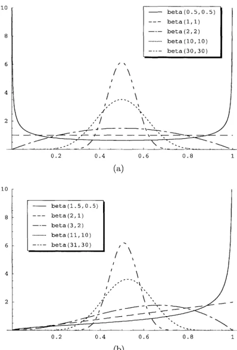
When initializing the Dirichlet counts, one must ensure that the Dirichlet counts for different network nodes do not conflict with one another. Consider the toy example pictured in Figure 3-2. In this Bayesian Network, the Dirichlet functions reduce to beta functions since each function only has two parameters. F21, the parameter

corresponding to the probability that X = 1, has a beta(1, 1) distribution, which is

similar to observing X = 1 once and X = 2 once during a total of two observations.

Fx2, the parameter corresponding to X = 2, is defined be 1 - Fx, because the sum

of the PMF parameters must equal one. Fy, has a beta(1, 1) distribution when

X = 1 and a beta(1, 0) distribution when X = 2, which is similar to observing

(X, Y) = (1, 1), (X, Y) = (1, 2), and (X, Y) = (2, 1) in three observations. Fy2 again

equals 1 - Fyj. In this case, the number of observations used to set beta counts for the X and Y parameters differ. This discrepancy can cause undesirable results as the Dirichlet counts are updated based on incoming information [10]. To avoid these complications, one must initialize the Dirichlet counts so that they are self-consistent, i.e., so that the sum of the counts assigned to each node is the same, and the counts can all be drawn from the same set of observations. When a Bayesian Network has self-consistent Dirichlet counts, the network is said to have an equivalent sample size equal to the sum of the Dirichlet counts assigned to a particular node. For example, if Fx, received a beta(2, 1) distribution in Figure 3-2, then the conflict would be removed, and the network would have an equivalent sample size of 2 + 1 = 3. For a

more rigorous exploration of equivalent sample sizes, refer to [10].

In addition to ensuring that the Dirichlet counts are initialized consistently, one should consider how their initial values will affect the speed with which the Bayesian Network adapts to new information. Since the PMF parameters are set to the ex-pected values of the underlying Dirichlet distributions, many different Dirichlet dis-tributions can result in the same PMF. If we again consider Dirichlet disdis-tributions with two parameters, all of the distributions pictured in Figure 3-3a result in the same PMF since they all have the same expected value. More specifically, suppose Z is akin to a Bernoulli random variable, and Z equals 1 with probability fi = E[F] and

Dirichiet Ditribution Dirichlet Ditribution beta(1, 1) If X = 1, beta(l,1) If X = 2, beta(1,0) X - Y P(Y = 11X = 1)= 0.5 P(X= 1)= 0.5 P(Y = 21X = 1)= 0.5 P(X =2)= .5 _{P(Y= IX = 2)= 1} PMF PMF P(Y = 21X = 2)=O

Figure 3-2: A Bayesian Network example that does not exhibit an equivalent sample size.

2 with probability f2 = E[F2] = 1 - fi. Assume that the beta(ai, a2) plots in Figure

3-3a now represent probability distribution for the random variable F1. In all cases,

fi = f2 = 0.5, since the beta distributions all have an expected value of 0.5. Each beta distribution, however, results in a different posterior distribution when certain data observations are made. Suppose we take each of the beta distributions in Figure

3-3a to be a prior distribution of F1, and we calculate the posterior distributions

after observing a new sample of Z. If we observe that Z = 1, the resulting posterior

distributions are pictured in Figure 3-3b. When the original beta parameters were

less than 1, observing that Z = 1 makes fi very close to 1 and f2 = 1 - fi very close

to 0. Alternatively, when the original beta parameters were both one, the prior is

uniform and fi becomes = 0.67, a value much closer to its a priori value of 0.5.

For the final two cases, fi stays very close to 0.5, because a more significant amount

of prior evidence indicates that fi and f2 are equal. Thus, by setting the a priori

Dirichlet counts in different ways, we can change how quickly the PMF parameters adapt to new data. The learning algorithms presented in the next section experiment

10 r 8 6 4 2

/

Figure 3-3: Examples of two-parameter Dirichlet distributions, otherwise known as beta distributions. - beta(0.5,0.5) --- beta(1,1) -- beta(2,2) --- ---- beta(10,10) beta (30, 30) \I

3.3

Learning Algorithms

In the medical setting, one wants to incorporate knowledge gained from medical ex-perts, general population statistics, and current patient data. An ideal Bayesian Net-work should rely on well-established information about the general population, while still adapting to the current patient. The learning, or training, algorithms presented in this section perform distribution parameter learning by relying on different ways of setting and constraining Dirichlet parameters to affect how quickly a Bayesian net-work adapts to new information and how strongly it depends on previously obtained history.

We can set a Bayesian Network's probability parameters using some combina-tion of pre-training initializacombina-tion, batch learning, and sequential learning. During pre-training initialization, we set the Dirichlet counts based on expert opinion and previous experience. In batch learning, we use information from previously acquired patient data to set or update the Dirichlet counts all at once. During sequential learning, we use incoming patient data, either one point at a time or several points at a time, to continuously update the Dirichlet counts based on recently acquired patient data.

The training algorithms presented in this section represent different ways of com-bining batch and sequential learning approaches to vary the amount and type of information stored in the network's probability distributions. We us these method-ologies to create networks that incorporate both persistent and transient memory components.

3.3.1

Batch Learning

During batch learning, the network receives all of the training data at once, cal-culates a single set of posterior Dirichlet distributions, and uses the same resulting PMFs and conditional PMFs every time that the network performs inference in the future. In other words, the network memory is persistent, and the Bayesian Network's probability distribution remains stationary.

Whenever we perform batch learning in this thesis, we precede the batch learn-ing by a pre-trainlearn-ing initialization step. Durlearn-ing this step, the Dirichlet counts are initialized uniformly so that the network has an equivalent sample size of 1. Since all nodes are modeled using five-level multinomial random variables, Dirichlet counts for nodes with no parents are initially set to 0.2, and Dirichlet counts for nodes with two parents initially equal 0.008. This means that all a priori PMFs and conditional PMFs are uniform, but as soon as the network receives training data, it immediately assigns an extremely low probability to values not appearing in the observed data set. This mirrors the beta(0.5, 0.5) case presented in Figure 3-3a.

During learning, the batch algorithm computes histograms for each set of child and parent nodes to count the number of times that different value combinations appear within the training data set. In the Bayesian Network model pictured in Figure 3-1, the learning algorithm independently computes histograms for TPR, HR, and SV, the nodes with no parents. The algorithm then adds the histogram results to the initial Dirichlet counts to obtain the updated Dirichlet counts. It then computes joint histograms for each set of {TPR, CO, BP} and {HR, SV, CO} values, and adds the appropriate histogram count to each of the corresponding initial Dirichlet counts. In this manner, it obtains updated Dirichlet counts for BP and CO, respectively. The algorithm sets each PMF parameter to the expected value of the appropriate updated Dirichlet distribution as explained in Sections 3.1 and 3.2. Once the updated PMF parameters are calculated, the training is complete. Each time the network is subsequently used for inference, the network uses this same set of PMF parameters.

3.3.2

Sequential Learning with Transient Memory

During sequential learning, the posterior distributions are recalculated every time that the network obtains a new piece of training data. In pure sequential learning, histograms are first computed on the new piece of training data in the same way as described above. The histogram values are again added to the Dirichlet priors to obtain the updated Dirichlet counts. The updated Dirichlet counts then become the Dirichlet priors used the next time the network receives another set of training