HAL Id: inria-00096807
https://hal.inria.fr/inria-00096807v2
Submitted on 24 Apr 2007HAL is a multi-disciplinary open access archive for the deposit and dissemination of sci-entific research documents, whether they are pub-lished or not. The documents may come from
L’archive ouverte pluridisciplinaire HAL, est destinée au dépôt et à la diffusion de documents scientifiques de niveau recherche, publiés ou non, émanant des établissements d’enseignement et de
Intersection and self-intersection of surfaces by means of
Bezoutian matrices
Laurent Busé, Mohamed Elkadi, André Galligo
To cite this version:
Laurent Busé, Mohamed Elkadi, André Galligo. Intersection and self-intersection of surfaces by means of Bezoutian matrices. Computer Aided Geometric Design, Elsevier, 2008, 25 (2), pp.53-68. �10.1016/j.cagd.2007.07.001�. �inria-00096807v2�
Intersection and self-intersection of surfaces
by means of Bezoutian matrices
L. Bus´e
a,∗ , M. Elkadi
b, A. Galligo
b,
aGalaad, INRIA Sophia Antipolis, 2004 Route des Lucioles, 06902 Cedex France. bLaboratoire J-A. Dieudonn´e, Universit´e de Nice, 06108 Cedex 2 France.
Abstract
The computation of intersection and self-intersection loci of parameterized surfaces is an important task in Computer Aided Geometric Design. We address these prob-lems via four resultants with separated variables; two of them are specializations of general multivariate resultants and the two others are specializations of deter-minantal resultants. We give a rigorous study in these four cases and provide new formulas in terms of Bezoutian matrix.
Key words: Algebraic surfaces, intersection locus, self-intersection locus,
resultants, Bezoutian.
1 Introduction
A common representation of surfaces in Solid Modeling and Computer Aided Geometric Design (CAGD) uses parameterized patches, i.e. images of maps of the form Φ : [0, 1] × [0, 1] → R3 (u, v) 7→ Φ(u, v) = Ã Φ1(u, v) Φ0(u, v) ,Φ2(u, v) Φ0(u, v) ,Φ3(u, v) Φ0(u, v) ! (1) where Φ0, Φ1, Φ2, Φ3are polynomials with real coefficients and bi-degree (m, n).
When Φ0(u, v) is a non-zero constant (independent of u and v), Φ is called ∗ Corresponding author.
Email addresses: lbuse@sophia.inria.fr (L. Bus´e), elkadi@math.unice.fr
a polynomial map, otherwise Φ is called a rational map. These patches are encountered in many applications [10], and spline surfaces are made by gluing them together.
There are many articles presenting methods and algorithms to intersect two patches [24,20,15,23] and to compute self-intersections loci [13,21,25,27,26]. These operations still need to be improved and computer algebra techniques can help. Among them, generalized resultant (for instance sparse resultant) techniques have been successfully employed [18,19,7].
The computation of self-intersection of a patch or intersection of two patches are important problems in CAGD; they were the main topics of the European project GAIA II [12]. Several strategies have been developed to address these problems: either via multivariate resultants [7], or via special case study [14], or via approximate implicitization [9,26], or via numerical methods [13]. Numerical methods algorithms are very efficient, however they often rely on samplings, and have the weakness common to these techniques: if the size of a loop in the (self-)intersection locus is smaller than the step-size of the sampling, it might become invisible and the program is unable to compute it. There are heuristics to choose the step-size, but they do not really overcome this difficulty.
Therefore, symbolic (or semi-numeric) methods are essential in order to solve completely these tasks. For that purpose, the parameterizations should be also algebraic. The most commonly used algebraic representations in CAGD are the so-called NURBS and particularly the polynomial patches.
In this paper, we will present new tools developed for this purpose. Namely specific sparse resultants and corresponding Bezoutian formulas allowing to compute, in each case presented below, a bivariate polynomial which is the equation of a plane projection of the double points locus. This polynomial is represented as the determinant of a small matrix, and thus it is useful for further post-processing.
For this setting, we prepare the equations for the elimination procedure in order to get a special format that we call with separated variables. Then we show that the obtained systems have nice properties that we further study and exploit.
We construct an unmixed bivariate resultant Res(P1, P2, P3) where the three
polynomials Pi(x, y) = fi(x) − gi(y), and apply it to the computation of
im-plicit equations of self-intersection and intersection loci of polynomial surfaces which is an important task in CAGD and Solid Modeling. In practice, this re-sultant is computed via a Bezoutian matrix, and it is related to (but different from) the toric resultant studied in [19,18]. In the case of rational surfaces,
we will use an anisotropic resultant to address the intersection problem and a determinantal resultant in the presence of base points to address the self-intersection problem. For each case, we show how to build a square matrix (namely a Bezoutian matrix) whose determinant is the expected resultant. We implemented our algorithms in Maple; an illustration and comparisons with the Maple package bires written by Amit Khetan are presented. We will show that the size of the matrix used in our approach to compute the different resultants are smaller than those given by Khetan’s method [18]. The methodology that we will use along this paper to obtain an elimination formula adapted to our special situations can be summarized as follows. Start-ing from a given polynomial system E, the first step is to ”homogenize” it (i.e. to embed it into an irreducible projective variety) with the condition that the obtained homogeneous system Eh do not have base-points. Then, by the
gen-eral theory of resultants, this system can be seen as a particular instance of a general resultant which is not identically zero. Moreover, the particular in-stance is always geometrically irreducible because, due to the hypothesis that
Eh is base-point free, the incidence variety is a vector bundle. However, it need
not to be algebraically reduced, but this property can be shown through well chosen specializations. This approach will be applied to the four different cases corresponding respectively to intersection and self-intersection of polynomial and rational parameterizations.
The paper is organized as follows. The next section provides a short overview on the Bezoutian matrix and its main property. In section 3, we precise the applications in CAGD and set the equations and the elimination problems for intersection and self-intersection. In section 4, we go back to our main CAGD applications and make explicit how our resultants can be used. We sketch also the algorithms and present examples. Sections 5 and 6 are more theoretical and they contain the proofs of our results. In section 5, we prove that in our situation, the specialization process is valid and that resultants (which are anisotropic) can be computed by nice Bezoutian formulas. In section 6, we describe an adapted version of the determinantal resultant and prove that these resultants can also be computed by simple Bezoutian formulas.
2 Overview on the Bezoutian matrix
In this short section we recall a well known matrix construction to eliminate variables from polynomial systems. We will apply it to prove formulas for bivariate resultants that will be used to solve the intersection and the self-intersection problems that we address.
Definition 1 Let f0, . . . , fn be n + 1 polynomials in n variables x1, . . . , xn
with coefficients in a commutative ring R. The Bezoutian of f0, . . . , fn is the
following polynomial in 2n variables x1, . . . , xn, y1, . . . , yn:
Bezf0,...,fn(x; y) := ¯ ¯ ¯ ¯ ¯ ¯ ¯ ¯ ¯ ¯ ¯ f0(x) ∂1f0(x, y) · · · ∂nf0(x, y) ... ... ... ... fn(x) ∂1fn(x, y) · · · ∂nfn(x, y) ¯ ¯ ¯ ¯ ¯ ¯ ¯ ¯ ¯ ¯ ¯ (2) where ∂ifj(x, y) := fj(y1, . . . , yi−1, xi, . . . , xn) − fj(y1, . . . , yi, xi+1, . . . , xn) xi− yi . Set Bezf0,...,fn(x; y) = P
α,βcα,βxαyβ with cα,β ∈ R. Fixing an order on the
monomials, the matrix (cα,β)α,β whose rows are indexed by the yβ such that
there exists α with cα,β 6= 0, and columns are indexed by the xα such that there
exists β with cα,β 6= 0, is called the Bezoutian matrix of f0, . . . , fn.
Notice that we can substitute x by y in the first column of the determinant Bezf0,...,fn(x; y) since fj(x) − fj(y) =
Pn
i=1(xi− yi)∂ifj(x, y). Observe also that
the Bezoutian matrix does not have a null row or a null column.
The Bezoutian matrix is an interesting tool in elimination theory because it allows to eliminate several variables at once in polynomial systems. More pre-cisely, suppose given a system f0(c, x) = · · · = fn(c, x) = 0 where c denotes a
collection of parameters and x denotes a collection of variables. Then, under suitable conditions of genericity [5, Theorem 2.2] it can be shown that there exists an irreducible polynomial in the parameters c which vanishes for a value
c0 of c if and only if the zero locus of f0(c0, x) = · · · = fn(c0, x) = 0 is strictly
larger than the zero locus of f0(c, x) = · · · = fn(c, x) = 0. This irreducible
polynomial is called the generalized resultant of f0(c, x), . . . , fn(c, x) with
re-spect to the variables x. Moreover it divides the determinant of any maximal minor of the Bezoutian matrix of f0(c, x), . . . , fn(c, x) [5, Theorem 3.4] (see also
[7, Theorem 3.7] for general statements). Therefore, if ∆(c) stands for the de-terminant of a maximal minor of the Bezoutian matrix of f0(c, x), . . . , fn(c, x),
then the vanishing of ∆ at a given value c0 of c is a necessary condition for
the vanishing of the generalized resultant of f0(c, x), . . . , fn(c, x) at c0. In
gen-eral, this condition is not sufficient; for instance, in the univariate case the determinant of the Bezoutian matrix of two polynomials with different de-grees differs from their resultant by a power of the leading coefficient of one of these polynomials. We refer the reader to [5, §4] for more examples and illustrations.
In this paper, we will consider four special classes of bivariate resultants for which we will prove that the determinants of the associated Bezoutian matrices
are exactly equal to the corresponding generalized resultants.
3 The main results
In this section we state four theorems addressing two important tasks in CAGD: the intersection and the self-intersection problems for polynomial and rational surfaces. The proofs of these results are rather technical as they re-quire some knowledge in algebraic geometry and rely on the use of specific resultants; they will be given in sections 5 and 6. Note also that the condition
sufficiently generic required in the following results will also be completely
described at that time.
3.1 Intersection problem
First we describe a particular projection of the pre-image curve (i.e the curve in the parameter space which maps to the intersection locus). We consider the intersection of two patches S1 and S2 given by parameterizations Φ(u, v) and
Ψ(s, t) with the same features as (1) that we view in the projective space P3.
The set S1∩ S2 corresponds to the quintuple of parameters (u, v, s, t, λ), with
λ 6= 0, such that Φ(u, v) = λΨ(s, t). This set form a curve C in R5 that we can
describe (i.e. give the topology and witness points on each component) via a well chosen projection on a plane
C1 = {(u, t) : ∃ (v, s, λ) with λ 6= 0 and Φ(u, v) = λΨ(s, t)}.
Our geometric task is equivalent to describe the curve C1. Its implicit
equa-tion is obtained by eliminating v, s, λ in the system Φ(u, v) = λΨ(s, t) of 4 equations defining C.
In the polynomial case (i.e. Φ0(u, v) = Ψ0(s, t) = 1), the question reduces to
the elimination of 2 variables v and s in a system of 3 polynomial equations in 4 variables (there is no λ).
Theorem 2 (see subsection 5.1) Suppose given two sufficiently generic
pa-rameterized polynomial surfaces of bi-degree (m, n):
(u, v) 7→³Φ1(u, v), Φ2(u, v), Φ3(u, v)
´ ,
(s, t) 7→³Ψ1(s, t), Ψ2(s, t), Ψ3(s, t)
´ .
The implicit equation of the projection of their intersection locus onto the plane (u, t) equals the determinant of the mn × mn Bezoutian matrix, given by the formula (2), of Φ1(u, v) − Ψ1(s, t), Φ2(u, v) − Ψ2(s, t), Φ3(u, v) − Ψ3(s, t)
viewed as polynomials in v and s.
In the rational case, we have the following result:
Theorem 3 (see subsection 6.1) Suppose given two sufficiently generic
pa-rameterized rational surfaces of bi-degree (m, n):
(u, v) 7→ Ã Φ1(u, v) Φ0(u, v) ,Φ2(u, v) Φ0(u, v) ,Φ3(u, v) Φ0(u, v) ! , (s, t) 7→ Ã Ψ1(s, t) Ψ0(s, t) ,Ψ2(s, t) Ψ0(s, t) ,Ψ3(s, t) Ψ0(s, t) ! .
The implicit equation of the projection of their intersection locus onto the plane (u, t) equals the determinant of the mn × mn matrix B(u, t) defined by
UB(u, t)Vt= 1 (v − v1)(s − s1) ¯ ¯ ¯ ¯ ¯ ¯ ¯ ¯ ¯ ¯ ¯ ¯ ¯ ¯ Φ0(u, v) Φ0(u, v1) Ψ0(s, t) Ψ0(s1, t) Φ1(u, v) Φ1(u, v1) Ψ1(s, t) Ψ1(s1, t) Φ2(u, v) Φ2(u, v1) Ψ2(s, t) Ψ2(s1, t) Φ3(u, v) Φ3(u, v1) Ψ3(s, t) Ψ3(s1, t) ¯ ¯ ¯ ¯ ¯ ¯ ¯ ¯ ¯ ¯ ¯ ¯ ¯ ¯
where U and V denote the monomial vectors
U := [sivj, i = 0 . . . m − 1, j = 0 . . . n − 1], V := [s1iv1j, i = 0 . . . m − 1, j = 0 . . . n − 1].
Observe that UB(u, t)Vt in Theorem 3 is a polynomial in v, v
1, s, s1, u, t.
3.2 Self-intersection problem
We start with a parameterization Φ given by (1) that we view in P3 and, as
in the previous subsection, we will describe a well chosen projection of the pre-image curve of the self-intersection locus.
The set of double points of Φ can be characterized by a curve
in R5. It can also be described in a simpler way by a curve of its well chosen
projection (generically 1 to 1) C1 on R2:
C1 = {(u, v); ∃ (k, l, λ) : (k, l) 6= 0, λ 6= 0, and Φ(u, v + k) = λΦ(u + l, v)}.
Our geometric task is equivalent to describe the curve C1. Its implicit equation
is obtained by the elimination of l, k, λ in the system of 4 equations defining
C1.
If the variables u, v are fixed, we remark that the point (k, l, λ) = (0, 0, 1) is a base-point (i.e. a solution which is independent of u and v) of the system Φ(u, v + k) − λΦ(u + l, v) = 0 defining C1. We will exploit this observation to
develop an adapted resultant for the self-intersection problem in subsections 5.2 and 6.2.
In the polynomial case, we have the following result:
Theorem 4 (see subsection 5.2) Suppose given a sufficiently generic
pa-rameterized polynomial surface of bi-degree (m, n):
(u, v) 7→³Φ1(u, v), Φ2(u, v), Φ3(u, v)
´ .
The implicit equation of the projection of its self-intersection locus onto the plane (u, v) equals the determinant of the (mn − 1) × (mn − 1) Bezoutian matrix B(u, v) defined by the formula (2):
UB(u, v)Vt = Bez
Φ1(u,v+k)−Φ1(u+l,v),Φ2(u,v+k)−Φ2(u+l,v),Φ3(u,v+k)−Φ3(u+l,v)(k, l; k1, l1)
with U :=hlikj, (i, j) ∈ {0, . . . , m − 1} × {0, . . . , n − 1} \ {0, 0}i, and
V :=hl1ik1j, (i, j) ∈ {0, . . . , m − 1} × {0, . . . , n − 1} \ {0, 0}
i .
In the rational case, we have:
Theorem 5 (see subsection 6.2) Suppose given a sufficiently generic
pa-rameterized rational surface of bi-degree (m, n):
(u, v) 7→ Ã Φ1(u, v) Φ0(u, v) ,Φ2(u, v) Φ0(u, v) ,Φ3(u, v) Φ0(u, v) ! .
The implicit equation of the projection of its self-intersection locus onto the plane (u, v) equals the determinant of the (mn − 1) × (mn − 1) Bezoutian
matrix B(u, v) defined by the formula (2): UB(u, v)Vt = 1 (k − k1)(l − l1) ¯ ¯ ¯ ¯ ¯ ¯ ¯ ¯ ¯ ¯ ¯ ¯ ¯ ¯ Φ0(u, v + k) Φ0(u, v + k1) Φ0(u + l, v) Φ0(u + l1, v) Φ1(u, v + k) Φ1(u, v + k1) Φ1(u + l, v) Φ1(u + l1, v) Φ2(u, v + k) Φ2(u, v + k1) Φ2(u + l, v) Φ2(u + l1, v) Φ3(u, v + k) Φ3(u, v + k1) Φ3(u + l, v) Φ3(u + l1, v) ¯ ¯ ¯ ¯ ¯ ¯ ¯ ¯ ¯ ¯ ¯ ¯ ¯ ¯
where U and V denote the monomial vectors
U :=hlikj, (i, j) ∈ {0, . . . , m − 1} × {0, . . . , n − 1} \ {0, 0}i, V :=hl1ik1j, (i, j) ∈ {0, . . . , m − 1} × {0, . . . , n − 1} \ {0, 0}
i .
Notice that UB(u, v)Vt in Theorem 5 is a polynomial in k, k
1, l, l1, u, v.
4 Comments and illustrations
The four theorems given in Section 3 are parts of a general approach to the intersection and self-intersection problems of algebraic surfaces that we now illustrate. For this purpose, we focus on the polynomial self-intersection prob-lem; the three other cases can be treated similarly.
Consider a surface given by (u, v) ∈ R2 7→³Φ
1(u, v), Φ2(u, v), Φ3(u, v)
´ ∈ R3
a polynomial parameterization of bi-degree (m, n) and define the polynomials
Pi(u, v, l, k) := Φi(u, v + k) − Φi(u + l, v) , i = 1, 2, 3,
of bi-degree (m, n) in the variables (l, k) with polynomial coefficients in (u, v) of bi-degree (m, n). Set
R(u, v) := Res³P1(u, v, l, k), P2(u, v, l, k), P3(u, v, l, k)
´
where the right hand side in this equality is a resultant operator that will be precised in subsection 5.2. In order to draw the portion of the projection of the self-intersection curve of the parameterized surface, say D, contained in [0, 1]2, we should find a point on each of its connected components. A point on
a component crossing the border of the square is easily found, so the difficulty is essentially concentrated on the internal loops. A common way to find a
point on such a loop is to compute all the critical points of D on an axis, e.g. the u-axis. This amounts to solve the bivariate system
R(u, v) = ∂R
∂u(u, v) = 0.
Once we get a point on each connected component of D contained in [0, 1]2, the
computer algebra part of the process is completed. Then a numerical marching algorithm can be used to compute the points (u, v + k, u + l, v) ∈ [0, 1]4 needed
to draw efficiently the pre-image curve or any of its plane projection. Note that a part of this process can be done by exploiting the kernel of the matrix which is used to compute the resultant R(u, v): for instance, if the couple (u, v) satisfies det³B(u, v)´ = 0, the vector U in Theorem 4 is in the kernel of the transpose of this matrix, so we can often obtain k and l as the quotient of two sub-minors of B(u, v) (see [4] for precise results).
An illustrative example. Let S be a parameterized surface of bidegree (2, 2) given by:
Φ1(s, t) := 2 s2 − t2s2− 5 t s2+ 7 s + 3 t2s + s t − 1 + 6 t2− 2 t,
Φ2(s, t) := 9 t2s2− 5 t s2+ 2 t2s + 4 s t + s − 7 t2+ 9 t,
Φ3(s, t) := t s2+ 2 s t − 2 t2.
To find the self-intersection locus of S, we express that this parameterization takes the same value at the two pairs of parameters (s, t) = (u, v + k) and (s, t) = (u + l, v). By Theorem 4 we form the Bezoutian of the three polynomi-als Φi(u, v+k)−Φi(u+l, v) for i = 1, 2, 3 (see Defintion 1) which can be written
as UB(u, v)Vt, with U = (l, k, lk) and V = (l
1, k1, l1k1). The matrix B(u, v)
is a 3 × 3 symmetric matrix of rank 3. Its determinant D(u, v) is of bi-degree (10, 10) in (u, v) and of total degree 14. At a generic point (u, v) on the curve
D(u, v) = 0, B(u, v) is of rank 2, therefore the kernel of tB(u, v) = B(u, v) is
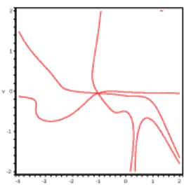
generated by a vector of type U. By Cramer’s rules, the entries of U are given by 2 × 2-minors of B(u, v), and after simplifications we find that l and k are given by two rational functions L(u, v) and K(u, v) of total degree 6 in (u, v). The graph of the curve D(u, v) = 0 is drawn in Figure 1. We notice that at the point (u, v) = (−1.05, −0.049) three local components of this curve intersect (see Figure 2). This can be checked by a formal algebraic computation. Now the graphs spanned by³u, v+K(u, v)´and by³u+L(u, v), v´, when (u, v) ranges on the graph of D(u, v), have also three local components intersecting at the two images of (u, v) = (−1.05, −0.049). Geometrically, on the surface S this corresponds to a singularity of the self-intersection curve similar to that of the Roman Steiner’s surface depicted in [8].
Fig. 1. A view of the double-point locus u 2 1 v -1 -3 0 0 -2 2 -2 -1 -4 1
Fig. 2. The projection of the double-point locus
Comparison with Khetan’s formulas. We end this section by comparing the four new elimination formulas we gave in Section 3 with the formulas given by Khetan to compute bivariate sparse resultants [18]. As far as we know, it is the lonely known matrix based method that produces exact elimination for-mulas. We implemented the constructions of matrices presented in Section 3 in Maple and used the Maple package bires written by Khetan. Khetan’s for-mulas are designed for bivariate resultants of any three polynomials, whereas our formulas are only available for bivariate resultants of polynomials with separated variables. However, since we took into account this particular struc-ture, our formulas compared most of the time favorably to the ones given by Khetan. Moreover, we observed sometimes that Khetan’s hybrid matrix is not full rank in some cases whereas the determinant of the matrix we propose gives exactly the projection of the intersection and self-intersection curve that we are looking for.
The following table presents some experiments. In the first column, we indicate the bi-degree of a randomly chosen rational surface. The second column gives the size of the matrix constructed by bires to compute the self-intersection locus of this rational surface, whereas the last column yields the size of the matrix obtained by Theorem 5 to solve the same problem.
Bi-degree Size of bires matrix Size of Bezoutian matrix
(2, 2) 11 × 11 3 × 3
(3, 2) 17 × 17 5 × 5
(3, 3) 27 × 27 8 × 8
The size of matrices obtained by Theorem 5 are significantly smaller than the ones given by Khetan’s approach. It follows that the computation of the self-intersection locus is highly increase because the more time-consuming step is by large the computation of determinants of these matrices (their construction is negligible compared to the computation of their determinants). Finally, we mention that Khetan’s formulas may fail to be non-zero; for instance, for randomly chosen rational surface of bi-degree (2,2), his approach returns a 11 × 11 matrix which is not full rank.
From now on, we focus on the proofs of the four theorems given in Section 3.
5 Bivariate resultants with separated variables
In this section, we suppose given three univariate polynomials of degree m ≥ 1
fi(x) := ai,0xm+ ai,1xm−1+ · · · + ai,m−1x + ai,m ∈ Z[ai,0, . . . , ai,m][x]
and three univariate polynomials of degree n ≥ 1
gi(y) := bi,0yn+ bi,1yn−1+ · · · + bi,n−1y + bi,n∈ Z[bi,0, . . . , bi,n][y].
Hereafter we will consider resultants of the three following bivariate polyno-mials with separated variables
Pi(x, y) := fi(x) − gi(y) ∈ A[x, y], i = 1, 2, 3,
where A := Z[(ai,j)i=1,2,3;j=0,...,m, (bi,j)i=1,2,3;j=0,...,n] denotes the universal
coef-ficients ring of these polynomials.
5.1 The dense case
This case will be applied to solve the intersection problem for polynomial surfaces.
To compute the classical resultant (sometimes called Macaulay’s resultant) of the polynomials P1(x, y), P2(x, y) and P3(x, y), we first need to
homoge-nize them to the projective space by introducing a new variable. But it is clear that this resultant is identically zero, since this homogenization pro-duces at least one base-point (i.e. a common root) in P2. To overcome this
problem, a natural idea is to change variables and compute the classical re-sultant of the polynomials P1(xn, ym), P2(xn, ym) and P3(xn, ym) which is not
identically zero. However, this resultant could be non reduced: it could be a power of an irreducible polynomial. As described in [16], its reduced part cor-responds to a resultant which is obtained by a (special) quasi-homogenization of P1(x, y), P2(x, y) and P3(x, y) to a weighted projective space aP2. We will
rely on this construction which has been fully studied in [16,17]. Recall that the weighted projective plane aP2 with a weight a = (a
0, a1, a2) ∈
N3over a field K is just the quotient space by the following relation: two points
(x0, x1, x2) and (y0, y1, y2) in K3\{0} are equivalent if there exists λ ∈ C∗ such
that (x0, x1, x2) = (λa0y0, λa1y1, λa2y2). For instance, the weighted projective
plane with the weight (1, 1, 1) is simply the usual projective plane. For more details on this topic we refer the reader to [1].
In general, the specialization of a given resultant operator to a set of non-generic polynomials may gives either an identically zero polynomial or a non irreducible polynomials on the restricted parameter space. However we will show that the specializations of some resultants are correct for our classes of non-generic polynomials but this requires a precise analysis and a rigorous proof, given below.
In our setting, introducing a new variable z, we homogenize P1(x, y), P2(x, y)
and P3(x, y) to the weighted projective space aP2 with homogeneous
coordi-nates (x, y, z) of weight (n, m, 1). We get, for i = 1, 2, 3, the quasi-homogeneous polynomials in A[x, y, z]: fih(x, z) := m X j=0 ai,jxm−jznj , gih(y, z) := n X j=0 bi,jyn−jzmj and Ph
i (x, y, z) := fih(x, z) − gih(y, z) of weight mn. We denote by ResaP2 the
anisotropic resultant of three polynomials in aP2. Hereafter we consider the
graded polynomial ring A with the usual grading: each of its variables has weight 1.
Proposition 6 The specialization ResaP2(P1h, P2h, P3h) of the anisotropic
re-sultant is a non-zero polynomial. It is homogeneous of degree mn with respect to the coefficients of each polynomial P1, P2 and P3, and hence has total degree
3mn. Moreover it is an irreducible element in A.
Proof. By specializing Ph
resul-tant R := ResaP2(P1h, P2h, P3h) equals 1 and it is hence non-zero. Moreover, by
the general result of [16,17], R is homogeneous with respect to the coefficients of each polynomial P1, P2 and P3 of degree mn.
The difficult point is to prove the irreducibility of R. We first prove that R is geometrically irreducible (i.e. it is a power of an irreducible polynomial). To do this we consider the incidence variety
W := {((x : y : z), (ai,j, bi,j)) : P1h = P2h = P3h = 0} ⊂aP2× A3(m+n+2)
and its two canonical projections π1 and π2onto the first and the second factor
respectively. By construction π1 gives W a structure of vector bundle overaP2
which is an irreducible variety. We deduce that W is itself an irreducible variety and therefore that its image by π2 is irreducible in the affine space A3(m+n+2).
This image has the same support than the zero locus of R and hence it follows that R is a certain power, say e, of an irreducible polynomial. Finally, to see that e = 1 we need to prove that the projection of W by π2 is bi-rational onto
its image. This done by considering the specialization φ defined, for generic
αi0s and βj0s by φ(P1h) = m Y i=1 (x − αizn) , φ(P2h) = n Y j=1 (y − βjzm) , φ(P3h) = xm− yn
which sends the anisotropic resultant R to
φ(R) = ResaP2( m Y i=1 (x − αizn), n Y j=1 (y − βjzm), xm− yn) = m,nY i,j=1 ResaP2(x − αizn, y − βjzm, xm− yn) = m,nY i,j=1 (αni − βjm).
(these two last equalities rely on properties of anisotropic resultants proved in [16]). Since the above product contains the irreducible and reduced factor
(α1− β1), e must be equal to 1. 2
We just proved the existence of a non-zero particular resultant which is adapted to our setting. The next task is to show that this resultant can be computed as the determinant of a certain square matrix, namely a Bezoutian matrix that we now describe.
polynomials P1(x, y), P2(x, y) and P3(x, y): BezP1,P2,P3(x, y; x1, y1) = − ¯ ¯ ¯ ¯ ¯ ¯ ¯ ¯ ¯ ¯ ¯
f1(x) − g1(y) f1(x)−fx−x11(x1) g1(y)−gy−y11(y1)
f2(x) − g2(y) f2(x)−fx−x21(x1) g2(y)−gy−y21(y1)
f3(x) − g3(y) f3(x)−fx−x31(x1) g3(y)−gy−y31(y1)
¯ ¯ ¯ ¯ ¯ ¯ ¯ ¯ ¯ ¯ ¯
and to deduce, after manipulations on the columns, that this Bezoutian has a particular symmetry property (which is not true in general), namely
BezP1,P2,P3(x1, y1; x, y) = BezP1,P2,P3(x, y; x1, y1).
The (x1, y1)-monomial support of this Bezoutian (i.e. the set of monomials
x1iy1j having non-zero coefficients) is {0, . . . , m−1}×{0, . . . , n−1}, and have
hence exactly mn elements. By the symmetry property, the (x, y)-monomial support is the same. Therefore the Bezoutian matrix B of P1, P2, P3 is, in this
case, a square matrix of size mn and we have:
Theorem 7 The determinant of the Bezoutian matrix B of P1, P2, P3 equals
the anisotropic resultant ResaP2(P1h, P2h, P3h) up to a sign1 in A.
Proof. From the discussion in Section 2, ResaP2(P1h, P2h, P3h) divides det(B).
Moreover, it is easy to see by Definition 1 that each entry of B is a polynomial in A which has total degree 3 and is homogeneous of degree 1 with respect to the coefficients of each polynomial P1, P2 and P3. Therefore, det(B) ∈
A is homogeneous with respect to the coefficients of each P1, P2 and P3 of
degree mn. Now, if det(B) is non-zero, it equals the anisotropic resultant ResaP2(P1h, P2h, P3h) up to a non-zero constant. Considering the specialization
φ defined by φ(P1) = xm, φ(P2) = yn and φ(P3) = 1, it is easy to check that
φ³BezP1,P2,P3(x, y; x1, y1) ´ = xm− xm1 x − x1 ×yn− y1n y − y1 ,
and that φ(det(B)) = ±1. So det(B) 6= 0 and the theorem is proved. 2
Note that, in more general setting, other formulations of the anisotropic re-sultant as a determinant of a square matrix has already been established in [17], and also in [18] as a sparse resultant. Theorem 7 is a simple expression in the particular case of polynomial systems with separated variables.
1 It is possible to fix the sign in this equality by requiring an ordering on the
5.2 The residual case
This case is adapted to the determination of self-intersection loci of polynomial surfaces.
We keep the notations of the subsection 5.1, but now we assume that the polynomials fi(x) and gi(x), for all i = 1, 2, 3, have the same constant term
(which is the case in the self-intersection problem), or in other words that
P1(0, 0) = P2(0, 0) = P3(0, 0) = 0.
Thus we have for i = 1, 2, 3, ai,m = bi,n and we view P1, P2 and P3 as
polyno-mials in A0[x, y], where A0 := Z[(a
i,j)i=1,2,3;j=0,...,m, (bi,j)i=1,2,3;j=0,...,n−1] is the
universal coefficients ring.
Similarly to the previous subsection, we introduce a new variable z and homog-enize the polynomials to the weighted projective space aP2 with coordinates
(x, y, z) of weight (n, m, 1). Then we have, for i = 1, 2, 3,
fh
i (x, z) := m
X
j=0
ai,jxm−jznj, ghi(y, z) := ai,mzmn+ n−1X
j=0
bi,jyn−jzmj
and Ph
i (x, y, z) := fih(x, z) − gih(x, z) are quasi-homogeneous of weight mn.
However, in this new setting, the anisotropic resultant ResaP2(P1h, P2h, P3h) is
degenerate because Ph
1, P2h and P3h vanish at the same point P := (0 : 0 : 1)
independently of their coefficients.
In order to deal with this base-point and get a non-identically zero resultant, we consider the blow-up πP :aP˜2 →aP2 of the weighted projective space along
the point P whose definition ideal is IP := (x, y), with exceptional divisor D.
Following techniques developed in [2,6] (see also [7] for a quick overview), we obtain the so-called residual resultant, and denoted by Resa˜P2(P1h, P2h, P3h). It
provides a necessary and sufficient condition for the zero locus in aP2 of the
system Ph
1(x, y, z) = P2h(x, y, z) = P3h(x, y, z) = 0 to be, scheme-theoretically,
strictly bigger than the point P . For more details, we refer the reader to [2,7,6]. Proposition 8 The residual anisotropic resultant Resa˜P2(P1h, P2h, P3h) is a
non-zero polynomial. It is homogeneous of degree mn − 1 with respect to the coef-ficients of each polynomial P1, P2, P3 and of total degree 3mn − 3. Moreover
it is an irreducible element in A0.
Proof. The proof is similar to that of Proposition 6, as it amounts to consider
an anisotropic residual resultant instead of a simple anisotropic one.
The geometric irreducibility of ˜R := ResaP˜2(P1h, P2h, P3h) follows from two facts.
projective irreducible variety. Second, the incidence variety ˜
W = {(˜t, (ai,j, bi,j)) : ˜P1h(˜t) = ˜P2h(˜t) = ˜P3h(˜t) = 0} ⊂aP˜2× A3(m+n+1)
is a vector bundle over aP˜2. Here ˜Ph
i denotes the virtual transform of Pih by
the blow-up πP (i.e. π∗P(Pih) divided only one time by the exceptional divisor
D).
As P is a smooth point in aP2, the self-intersection number R
a˜P2D2 of D
equals −1. Since each Ph
i is quasi-homogeneous of degree mn, the multi-degree
formula for residual resultants (see [2]) shows that ˜R is homogeneous, with
respect to the coefficients of each Pi, of degree mn +
R
aP˜2D2 = mn − 1.
Finally, to prove that ˜R 6= 0 and it is not a power of an irreducible
polyno-mial, we exhibit a specialization of P1, P2 and P3 such that the corresponding
specialization of ˜R is non-zero and contains an irreducible and reduced factor,
as we did in the proof of Proposition 6. For that purpose, we compute
ResaP˜2(x m−1Y i=1 (x − αizn), y n−1Y i=1 (y − βizm), xm − yn) = m−1,n−1Y i,j=1 (αn i − βjm). 2
Having defined the anisotropic residual resultant, we now describe how to compute it as the determinant of a Bezoutian matrix.
We proceed exactly as in the dense case, by considering the Bezoutian ma-trix of the polynomials P1, P2, P3. The only difference is that ai,m = bi,n for
i = 1, 2, 3, which implies that the (x, y)-monomial support (resp. the (x1, y1
)-monomial support) of this Bezoutian does not contain the )-monomial 1 = x0y0
(resp. 1 = x0
1y10) and hence contains only mn − 1 elements. Therefore, we get
a square matrix ˜B of size mn − 1 and we have:
Theorem 9 The determinant of the Bezoutian matrix ˜B of P1, P2, P3 is
ex-actly the residual anisotropic resultant Resa˜P2(P1h, P2h, P3h) up to a sign in A0.
Proof. From the discussion in Section 2, ResaP˜2(P1h, P2h, P3h) divides det(˜B). It
is straightforward to check that each entry of ˜B is a polynomial in A0which has
total degree 3 and is homogeneous of degree 1 with respect to the coefficients of each P1, P2 and P3. Therefore det(˜B) ∈ A0 is homogeneous with respect
to the coefficients of each polynomial P1, P2 and P3 of degree mn − 1. Now,
considering the specialization φ defined by φ(P1) = xm+ x, φ(P2) = yn and
φ(P3) = x − y, we obtain that φ
³
BezP1,P2,P3(x, y; x1, y1)
´
µxm− xm 1 x − x1 + 1 ¶ Ã yn+ (x − y)yn− yn1 y − y1 ! − (xm+ x) Ã yn− yn 1 y − y1 ! .
This implies that φ(det(˜B)) = ±1 and concludes the proof. 2
6 Bivariate determinantal resultants with separated variables With the strategy described in Section 3, the computation of the intersection locus of two rational surfaces requires the elimination of variables x, y, λ in a polynomial system of the form
φi(x) = λψi(y), i = 0 . . . 3 and λ 6= 0,
where the φi’s (resp. the ψi’s) are univariate polynomials in the variable x
(resp. y) of given degree m ≥ 1 (resp. n ≥ 1). This is equivalent to the fact that the 4 × 2 matrix defined by the φi’s and ψi’s has rank 1 at some point (x, y).
This leads to the notion of determinantal resultant introduced and studied in [2]. Therefore, to study the intersection and self-intersection problems for rational surfaces we need an extension of tools used in the polynomial case to the determinantal setting.
Introducing new variables ¯x and ¯y, we can put this system into a (bi)-projective
context to first eliminate the variable λ. Then, we eliminate the two couples of homogeneous variables (x, ¯x) and (y, ¯y) from the bi-homogeneous polynomial
system ³ φh 0(x, ¯x) : φh1(x, ¯x) : φh2(x, ¯x) : φh3(x, ¯x) ´ = ³
ψh0(y, ¯y) : ψh1(y, ¯y) : ψ2h(y, ¯y) : ψ3h(y, ¯y)´∈ P3,
where, for i = 0, 1, 2, 3, deg(φh
i) = m ≥ 1 and deg(ψhi) = n ≥ 1.
This elimination problem does not correspond to the projection of a complete intersection incidence variety, as in Section 5, then the previous theory of re-sultants does not apply. However, there is a generalization of the previous approach where the incidence variety is a determinantal one, and one can de-fine a determinantal resultant (see [3]). It turns out that this can be applied in our setting: this elimination problem fits into the class of determinantal poly-nomial systems (which is much larger than the class of complete intersection ones).
We re-formulate the elimination problem as the necessary and sufficient con-dition on the parameters of the polynomials φh
there exists a point ³(x : ¯x), (y : ¯y)´∈ P1× P1 which satisfies
rank
φ0(x, ¯x) φ1(x, ¯x) φ2(x, ¯x) φ3(x, ¯x) ψ0(y, ¯y) ψ1(y, ¯y) ψ2(y, ¯y) ψ3(y, ¯y)
< 2.
Let us fix the notations. From now on, we suppose given four univariate poly-nomials of degree m ≥ 1, i = 0 . . . 3,
φi(x) := ai,0xm+ ai,1xm−1 + · · · + ai,m−1x + ai,m ∈ Z[ai,0, . . . , ai,m][x]
and their corresponding homogenizations φh
i(x, ¯x) ∈ Z[ai,0, . . . , ai,m][x, ¯x], as
well as four univariate polynomials of degree n ≥ 1, i = 0 . . . 3,
ψi(y) := bi,0yn+ bi,1yn−1+ · · · + bi,n−1y + bi,n∈ Z[bi,0, . . . , bi,n][y]
and their corresponding homogenizations ψh
i(y, ¯y) ∈ Z[bi,0, . . . , bi,n][y, ¯y]. We
denote by A := Z[(ai,j)i=0,...,3;j=0,...,m, (bi,j)i=0,...,3;j=0,...,n] the universal
coeffi-cients ring of these polynomials.
We will use the theory of determinantal resultants developed in [3]. In partic-ular, we will provide new formulas to compute determinantal resultants with separated variables using Bezoutian matrices.
6.1 The dense case
Let us denote by X := P1× P1, O
X the vector bundle of rational functions
on X, and consider two vector bundles E := O4
X and F := OX(m, 0) ⊕
OX(0, n). Taking the coefficients of polynomials φi’s and ψi’s in C, this system
corresponds to a map of vector bundles on X, ρ : E → F , whose matrix is given by
M³(x, ¯x), (y, ¯y)´:=
φ0(x, ¯x) φ1(x, ¯x) φ2(x, ¯x) φ3(x, ¯x) ψ0(y, ¯y) ψ1(y, ¯y) ψ2(y, ¯y) ψ3(y, ¯y)
.
Following [3], the determinantal resultant associated to this morphism exists and corresponds to the necessary and sufficient condition on φi’s and ψi’s
coefficients so that there exists a point³(x0 : ¯x0), (y0 : ¯y0)
´
∈ P1×P1satisfying
rank M³(x0 : ¯x0), (y : ¯y0)
´ ≤ 1.
We denote this determinantal resultant, which is an element in A defined up to a sign, by ResX(M). In this case, we have the following proposition:
Proposition 10 The determinantal resultant ResX(M) is a non-zero
irre-ducible polynomial in A. Moreover, for each j ∈ {0, . . . , 3}, it is a homoge-neous polynomial with respect to the coefficients of φj and ψj of degree mn,
and it is hence a homogeneous element in A of degree 4mn.
Proof. First, we will justify the existence of ResX(M). Set H = Hom(E, F ).
Although the vector bundle H is not very ample on X, the proof of Theorem 1 in [3] applies. In this proof, the very ampleness hypothesis is used to show that the projection from the incidence variety W to the projectivized parameter space P(H):
W = {(x, φ) ∈ X × P(H) : rank(φ(x)) ≤ 1} → P(H)
is bi-rational onto its image (which is called the resultant variety). The ar-gument is the following: given a zero-dimensional sub-scheme z of P1× P1 of
degree two (that is two distinct points or a double point), the locus of matri-ces φ in P(H) of rank lower or equal to 1 on z is of co-dimension twice the co-dimension of matrices of rank lower or equal to 1 on only one smooth point (which is here 3). In our particular situation, this property remains true, even if H is not very ample.
To obtain the claimed partial degrees we use the intersection theory as devel-oped in [11]: given an integer j ∈ {0, . . . , 3} we know from [3] that the degree of ResX(M) with respect to the coefficients of φj and ψj equals the coefficient
of the monomial αj in the coefficient of t3 in the expansion of the series
− Q4 i=1(1 − αit) ct(F ) = − 1 ct(F ) (1 − (α1+ α2 + α3+ α4)t + · · · )
where ct(F ) denotes the Chern polynomial of F . We deduce that this degree
is exactly the degree of the coefficient of t2 in the series 1/c
t(F ). Denoting by
H1 (resp.H2) the class of the generic point in the first (resp. second) factor P1
of X, we have ct(F ) = ct ³ OX(m; 0) ´ ct ³ OX(0; n) ´ = (1 + mH1)(1 + nH2) = 1 + mH1+ nH2+ mnH1H2. It follows that 1 ct(F ) = 1 − c1(F )t + ³ c1(F )2− c2(F ) ´ t2+ · · ·
from which we obtain that the degree of ResX(M) with respect to the
Z Xc1(F ) 2− c 2(F ) = Z X(mH1 + nH2) 2− mnH 1H2 = Z 2mnH1H2− mnH1H2 = Z XmnH1H2 = mn. 2
Remark 11 We recall from [3] that ResX(M) is, for all (p, q) ∈ N2 such that
p ≥ 3m − 1 and q ≥ 3n − 1, the determinant of the following graded part of
the Eagon-Northcott complex
S[−3, −1](p−3m;q−n) ⊕ S[−2, −2](p−2m;q−2n) ⊕ S[−1, −3](p−m;p−3n) ∂2 −→ S[−2, −1]4 (p−2m;q−n) ⊕ S[−1, −2]4 (p−m;q−2n) ∂1 −→ S[−1, −1]6(p−m;q−n)−−→ S[0, 0]∧2ρ (p;q)
where S is the ring
S := (Z[(ai,j)i=0,...,3,j=0,...,m] ⊗ZZ[(bi,j)i=0,...,3,j=0,...,n]) ⊗Z(Z[x, ¯x] ⊗Z Z[y, ¯y])
which is equipped (via tensor products) with two (bi-graded) gradings that we denote by S[−, −](−,−). In particular, ResX(M) vanishes if and only if the
rank of the 9mn × 24mn matrix
S[−1, −1]6(2m−1;2n−1)−−→ S[0, 0]∧2ρ (3m−1;3n−1)
drops. Moreover, from this result we can deduce that ResX(M) ∈ A is
ho-mogeneous with respect to the coefficients of (φi)i=0,...,3 (resp.(ψi)i=0,...,3) of
degree 2mn.
We now turn to the computation of this determinantal resultant in our setting. We consider the four polynomials
Pi(x, y, λ) := φi(x) − λψi(y), i = 0 . . . 3,
and we compute the Bezoutian BezP0,...,P3(x, y, λ; x1, y1, λ1) which equals
−λ ¯ ¯ ¯ ¯ ¯ ¯ ¯ ¯ ¯ ¯ ¯ ¯ ¯ ¯
φ0(x) φ0(x)−φx−x01(x1) ψ0(y) ψ0(y)−ψy−y10(y1)
φ1(x) φ1(x)−φx−x11(x1) ψ1(y) ψ1(y)−ψy−y11(y1)
φ2(x) φ2(x)−φx−x21(x1) ψ2(y) ψ2(y)−ψy−y12(y1)
φ3(x) φ3(x)−φx−x31(x1) ψ3(y) ψ3(y)−ψy−y13(y1)
¯ ¯ ¯ ¯ ¯ ¯ ¯ ¯ ¯ ¯ ¯ ¯ ¯ ¯ .
This Bezoutian does not depend on the variable λ1, and we can eliminate λ from it by defining Bez0 P0,...,P3(x, y; x1, y1) := BezP0,...,P3(x, y, λ; x1, y1, λ1) λ .
It is clear that Bez0P0,...,P3(x, y; x1, y1) = BezP00,...,P3(x1, y1 : x, y). The (x1, y1
)-monomial support (and hence also its (x, y)-)-monomial support) of this Be-zoutian is {0 . . . m − 1} × {0 . . . n − 1}. Therefore we can construct a square matrix B0 of size mn from it and we have:
Theorem 12 The determinant of the matrix B0 equals to the determinantal
resultant ResX(M) in A up to a sign.
Proof. From the discussion in Section 2, ResX(M) divides det(B0). Since they
have the same degree as homogeneous elements in A, we deduce that the claimed result will be proved if we show that det(B0) equals ±1 for a given
specialization. For this, we consider the specialization ρ defined by
ρ(φ0) = xm, ρ(φ1) = 0, ρ(φ2) = 0, ρ(φ3) = 1,
ρ(ψ0) = 0, ρ(ψ1) = yn, ρ(ψ2) = 1, ρ(ψ3) = 0.
It is straightforward to check that ρ(det(B0)) = ±1 (the sign depends on the
ordering chosen on monomials to construct B0). 2
6.2 The residual case
With the same notations as in subsection 6.1, we now assume that for i = 0 . . . 3, the polynomials φi(x) and ψi(y) have the same constant term (which
is the case for the self-intersection problem); that is
φi(0) = ai,m = bi,n = ψi(0) for i = 0, 1, 2, 3.
The ring A0 := Z[(a
i,j)i=0,1,2,3;j=0,...,m, (bi,j)i=0,1,2,3;j=0,...,n−1] denotes the
univer-sal coefficients ring.
We remark that the determinantal resultant ResX(M) ∈ A0 in Proposition 10
is identically zero in this case because the matrix M is always of rank less or equal to 1 at P =³(0 : 1), (0 : 1)´∈ P1× P1. So, we are no longer considering
all the morphisms E → F , but only those having rank 1 at this point P . Similarly to what we did in subsection 5.2, we can overtake this difficulty by considering the blow-up πP : ˜X → X = P1 × P1 of X along P . Then the
morphism π∗
P(E) → π∗P(F ) have generically rank 2 outside the exceptional
divisor D and rank 1 on D. Therefore, for such a general morphism, the co-kernel Q fits in the exact sequence
π∗
P(E)|D → π∗P(F )|D → Q → 0
and is a vector bundle of rank 1 over D. It follows that the kernel ˜F of the
canonical surjective morphism π∗
P(F ) → Q → 0 is also a vector bundle2 over
˜
X and has the same rank than F . We have the exact sequence
0 → ˜F → π∗
P(F ) → Q → 0. (3)
It turns out that the morphism π∗
P(E) → πP∗(F ) factors through ˜F and the
residual determinantal resultant we are looking for is the determinantal re-sultant of vector bundles ˜E := π∗
P(E) and ˜F over ˜X. We will denote it by
ResX˜(M). It gives a necessary and sufficient condition so that the
determi-nantal locus in X corresponding to the condition rank
φ0(x, ¯x) φ1(x, ¯x) φ2(x, ¯x) φ3(x, ¯x) ψ0(y, ¯y) ψ1(y, ¯y) ψ2(y, ¯y) ψ3(y, ¯y)
< 2
is, scheme-theoretically, strictly bigger than the point P .
Proposition 13 The residual determinantal resultant ResX˜(M) is a non-zero
irreducible polynomial in A0. Moreover, for each integer j ∈ {0, . . . , 3}, it is
homogeneous with respect to the coefficients of φj and ψj of degree mn − 1,
and hence it is a homogeneous element in A0 of degree 4mn − 4.
Proof. The proof of the irreducibility of ResX˜(M) is exactly the same than the
one given in Proposition 10 using the general theory developed in [3]. Given an integer j ∈ {0, . . . , 3}, the degree of ResX˜(M) with respect to the coefficients
of φj and ψj equals the degree of the coefficient of t2 in the series 1/ct( ˜F ).
From the exact sequence (3) we deduce that ct( ˜F )ct(Q) = ct(F ). Moreover,
using the definition of M and Q we have Q ' OD, so we deduce that
1 ct( ˜F ) =ct(OD) ct(F ) = 1 ct(F )ct(OX˜(−D)) = 1 ct(F ) × 1 1 − Dt =³1 − c1(F )t + (c1(F )2− c2(F ))t2+ · · · ´ ³ 1 + Dt + D2t2+ · · ·´.
Hence the degree of ResX˜(M) with respect to the coefficients of φj and ψj
2 this is a consequence of the fact that Q has rank 1. The construction of ˜F is
known as an elementary transformation of the vector bundle F (see [22] for more details).
equals Z ˜ XD 2− c 1(F )D + c1(F )2− c2(F ) = Z ˜ Xc1(F ) 2 − c 2(F ) + Z ˜ XD 2 = mn − 1.
As a consequence, the residual determinantal resultant ResX˜(M) is an
homo-geneous element in A0 of degree 4(mn − 1) = 4mn − 4. 2
To compute this residual determinantal resultant we use, as before, Bezoutian matrices. With the same notations and computations as in subsection 6.1, we build the Bezoutian matrix B0 of size mn × mn. However in this more
particular setting, the couple (0, 0) (associated to the monomial 1) is not in the (x, y)-monomial support and not also in the (x1, y1)-monomial support. In
this way, we consider the mn − 1 × mn − 1 sub-matrix ˜B0 of B0 corresponding
to erase the row and the column which defines the monomial 1.
Theorem 14 The determinant of the matrix ˜B0 equals the residual
determi-nantal resultant ResX˜(M) in A0 up to a sign.
Proof. From the discussion in Section 2, ResX˜(M) divides det( ˜B0). Since these
two polynomials have the same degree as homogeneous elements in A0, we
deduce that the claimed result is proved if we show that det( ˜B0) equals ±1 for
a given specialization. To do this, we consider the specialization ρ defined by
ρ(φ0) = xm+ x, ρ(φ1) = 0, ρ(φ2) = x, ρ(φ3) = 1,
ρ(ψ0) = 0, ρ(ψ1) = yn, ρ(ψ2) = −y, ρ(ψ3) = 1,
and it is straightforward to check that ρ(det(˜B0)) = ±1 (the sign depends on
the ordering chosen on monomials to construct the matrix ˜B0). 2
7 Conclusion
In this paper we presented a re-formulation of computer algebra problems related to the determination of the self-intersection and intersection loci of polynomial surfaces patch and in the more general case of rational patches used for NURBS. We gave simple and efficient formulas to compute the implicit equation of certain projections of these loci. The next step is to study a numeric adaptation of the original approach described in this paper.
Acknowledgments
This work was partially supported by the French Research Agency (ANR Gecko) and the European Network of Excellence Aim@Shape (IST NoE 506766). The authors thanks Andr´e Hirschowitz for helpful discussions on elementary transformations of vector bundles.
References
[1] M. Beltrametti and L. Robbiano. Introduction to the theory of weighted projective spaces. Exposition. Math., 4(2):111–162, 1986.
[2] L. Bus´e. Etude du r´esultant sur une vari´et´e alg´ebrique. PhD thesis, Universit´e de Nice Sophia-Antipolis, 2001.
[3] L. Bus´e. Resultants of determinantal varieties. J. Pure Appl. Algebra, 193(1-3):71–97, 2004.
[4] L. Bus´e and C. D’Andrea. Inversion of parameterized hypersurfaces by means of subresultants. In ISSAC 2004, pages 65–71. ACM, New York, 2004.
[5] L. Bus´e, M. Elkadi, and B. Mourrain. Generalized resultants over unirational algebraic varieties. J. Symbolic Comput., 29(4-5):515–526, 2000. Symbolic computation in algebra, analysis, and geometry (Berkeley, CA, 1998).
[6] L. Bus´e, M. Elkadi, and B. Mourrain. Resultant over the residual of a complete intersection. J. Pure Appl. Algebra, 164(1-2):35–57, 2001. Effective methods in algebraic geometry (Bath, 2000).
[7] L. Bus´e, M. Elkadi, and B. Mourrain. Using projection operators in computer aided geometric design. In Topics in algebraic geometry and geometric modeling, volume 334 of Contemp. Math., pages 321–342. Amer. Math. Soc., Providence, RI, 2003.
[8] A. Coffman, A. J. Schwartz, and C. Stanton. The algebra and geometry of Steiner and other quadratically parametrizable surfaces. Comput. Aided Geom.
Design, 13(3):257–286, 1996.
[9] T. Dokken. Approximate implicitization. In Mathematical methods for curves
and surfaces (Oslo, 2000), Innov. Appl. Math., pages 81–102. Vanderbilt Univ.
Press, Nashville, TN, 2001.
[10] G. Farin. Curves and surfaces for computer aided geometric design. Computer Science and Scientific Computing. Academic Press Inc., Boston, MA, third edition, 1993. A practical guide, With 1 IBM-PC floppy disk (5.25 inch; DD). [11] W. Fulton. Intersection theory, volume 2 of Ergebnisse der Mathematik
und ihrer Grenzgebiete (3) [Results in Mathematics and Related Areas (3)].
[12] GAIA II. European project. http://www.sintef.no/static/AM/gaiatwo/. [13] A. Galligo and J.-P. Pavone. A sampling algorithm for parametric surface
self-intersection. Preprint, 2006.
[14] A. Galligo and M. Stillman. The geometry of bicubic surfaces and splines. To appear in Journal of Symbolic Computation, 2006.
[15] M. Hosaka. Modeling of Curves and Surfaces in CAD/CAM. Springer-Verlag, New York, NY, 1992.
[16] J.-P. Jouanolou. Le formalisme du r´esultant. Adv. Math., 90(2):117–263, 1991. [17] J.-P. Jouanolou. R´esultant anisotrope, compl´ements et applications. Electron.
J. Combin., 3(2):Research Paper 2, approx. 91 pp. (electronic), 1996. The Foata
Festschrift.
[18] A. Khetan. The resultant of an unmixed bivariate system. J. Symbolic Comput., 36(3-4):425–442, 2003. International Symposium on Symbolic and Algebraic Computation (ISSAC’2002) (Lille).
[19] A. Khetan, N. Song, and R. Goldman. Sylvester A-resultants for bivariate polynomials with planar Newton polygons (extended abstract). In ISSAC 2004, pages 205–212. ACM, New York, 2004.
[20] S. Krishnan and D. Manocha. An efficient surface intersection algorithm based on lower-dimensional formulation. In ACM Transactions on Graphics, volume 16, pages 74–106, 1997.
[21] D. Lasser. Self-intersections of parametric surfaces. In Proceedings of the
International Conference on Engineering Graphics and Descriptive Geometry, Vienna Volume 1 pages 322-321, 1988.
[22] M. Maruyama. Elementary transformations in the theory of algebraic vector bundles. In Algebraic geometry (La R´abida, 1981), volume 961 of Lecture Notes
in Math., pages 241–266. Springer, Berlin, 1982.
[23] N. Patrikalakis. Surface-to-surface intersections. In IEEE Computer Graphics
and Applications, volume 13, pages 89–95, 1993.
[24] T. W. Sederberg and R. J. Meyers. Loop detection in surface patch intersections.
Comput. Aided Geom. Design, 5(2):161–171, 1988.
[25] W. C. T. Maekawa and N. M. Patrikalakis. Computation of self-intersections of offsets of bezier surface patches. Journal of Mechanical Design, ASME
Transactions, 119(2):275-283, 1997.
[26] J. B. Thomassen. Self-intersection problems and approximate implicitization. In
Computational methods for algebraic spline surfaces, pages 155–170. Springer,
Berlin, 2005.
[27] P. Volino and N. M. Thalmann. Collision and self-collision detection: Efficient and robust solutions for highly deformable surfaces. In D. Terzopoulos and D. Thalmann, editors, Computer Animation and Simulation’95, pages 55–65. Springer-Verlag, 1995.