Applied change of mean detection techniques for HVAC fault detection and diagnosis and power monitoring

(1)

Applied Change of Mean Detection Techniques

for HVAC Fault Detection and Diagnosis and

Power Monitoring

by

Roger Owen Hill

B.A., Political Science. Swarthmore College, 1989 B.S., Engineering. Swarthmore College, 1991

Submitted to the Department of Architecture in Partial Fulfillment of the Requirements for the Degree of

Master of Science in Building Technology at the

Massachusetts Institute of Technology June 1995

The author hereby grants to MIT permission to reproduce and to distribute publicly paper and electronic copies of this thesis document in whole or in part.

17

Signature of Author... ... ... Department of Architecture May 5, 1995 Certified by...

Professor Leslie K. Norord Thesis Supervisor

Accepted

by...

Professor Leon Glicksman

Chairman, Building Technology Group ;ASSACTHUsETTS INSTITUTE

OF TECHNOLOGY

JUL 251995

(2)

(3)

Applied Change of Mean Detection Techniques for HVAC Fault

Detection and Diagnosis and Power Monitoring

by

Roger Owen Hill

Submitted to the Department of Architecture on May 5, 1995 in partial fulfillment of the requirements for the Degree of Master of Science in

Building Technology

Abstract:

A signal processing technique, the detection of abrupt changes in a

time-series signal, is implemented with two different applications related to energy use in buildings. The first application is a signal pre-processor for an advanced electric power monitor, the Nonintrusive Load Monitor

(NILM), which is being developed by researchers at the Massachusetts

Institute of Technology. A variant form of the generalized likelihood ratio (GLR) change-detection algorithm is determined to be appropriate for detecting power transients which are used by the NILM to uniquely identify the start-up of electric end-uses.

An extension of the GLR change-detection technique is used with a second application, fault detection and diagnosis in building heating ventilation and air-conditioning (HVAC) systems. The method developed here analyzes the transient behavior of HVAC sensors to define conditions of correct operation of a computer simulated constant air volume HVAC sub-system. Simulated faults in a water-to-air heat exchanger (coil fouling and a leaky valve) are introduced into the computer model. GLR-based analysis of the transients of the faulted HVAC system is used to to uniquely define the faulty state. The fault detection method's sensitivity to input parameters is explored and further avenues for research with this method are suggested.

Thesis supervisor: Dr. Leslie K. Norford

(4)

(5)

Acknowledgements:

I would like to acknowledge the financial support received from ESEERCo,

and the wealth of assistance I have received from colleagues and friends. In particular, the sage advise, FORTRAN and HVACSIM+ troubleshooting and sane presence of David Lorenzetti can not be understated. Dr. Norford's patience, encouragement and dedication throughout my graduate career has been immensely appreciated.

I also thank Dr. Leeb for providing the impetus for this research; even

though, the ultimate result followed a different course. I appreciate the support of my HVACSIM+ team including: Mark DeSimone, Tim Salsbury and Phil Haves. The camaraderie of the rest of the Building Technology researchers, in particular: Kath Holden, Jimmy Su, Greg Sullivan, Mehmet Okutan, Kachi Akoma, Kristie Bosko and Chris Ackerman, provided conversational diversions when I most needed them.

I am also grateful for the encouragement from my parents and co-workers

at New England Electric who reminded me that a legitimate goal of graduate school is finishing the thesis.

Finally, none of this would have been possible without the spiritual support of my best friend and wife, Vida, whose unwavering faith in me and stabilizing presence maintained my sanity throughout my graduate school experience.

(6)

(7)

Chapter

1 INTRODUCTION

Increasingly the study of Building Technology is converging with Information Technology. The questions researchers encounter become 'What can a building tell me about itself?'; 'How do we acquire information from a building?' and 'How do we locate the important information once we wire the building for communication?'

Brief Problem Overview

This thesis examines aspects of the third question in response to previous research which address the other two. We look at a method of extracting relevant information from the overwhelming amounts of data which a well wired building can generate about itself. In the first of two related projects, we utilize a signal processing tool to identify relevant portions of time-series power data without wasting effort on the less important on data. The second project uses the same signal processing tool to not only locate relevant data, but also to analyze the state of an operating system.

More precisely, this thesis examines two issues of on-line information processing associated with energy use in buildings. Because of the recent expansion of digital control of their systems, buildings have become significant sources and consumers of time-series information. Electric utilities have recognized that the structures where we live and work are an exceptional medium for gathering a wealth of data about how we use energy. Building operators know that if they can get different systems within a building to communicate appropriate information, the building will operate more efficiently with greater comfort for the occupants. A significant obstacle for both the utilities and the building operators is gleaning the necessary and sufficient data from the flood of information which is available when the building is wired to communicate with its occupants and operators.

(12)

In Chapter 2 of this thesis we examine on-line analysis of electrical power data to further the development of a non-intrusive load monitor (NILM) for commercial applications. Briefly, the commercial NILM is an advanced electric consumption monitor which not only measures the energy consumed on a circuit, but also uses software to identify the type of device which is consuming the energy. For accurate end-use identification the NILM must analyze electric power use data at a very high rate. The end-use determination software, though elegantly designed, is computationally intensive. This combination of

rapid data acquisition and extensive computation makes the NILM susceptible to data overload; therefore, we develop a method to pre-process the power consumption data to determine the critical segments that the NILM must

analyze.

Chapter 3 of this thesis extends the use of the data processing technique (developed for the NILM) to the analysis of data from a building's heating ventilation and air-conditioning (HVAC) systems. The goal in Chapter 3 is to develop a fault detection and diagnosis methodology to isolate and identify

HVAC system failures or confirm correct operation.

1.1 Application 1: Non-Intrusive Load Monitors

Since the mid-1980's public utility regulators have persuaded electric utilities to encourage energy conservation among all of their customers. The theory behind this policy is that if the cost for conserving energy is less than the cost of supplying that energy to the customer, then the utility ought to help their customers conserve. The inducements which the regulators use to advance this policy include allowing utilities to recover their cost and even make profits from their conservation efforts by raising electricity rates. These rate increases involve a tremendous amount of money, and regulators and customers want to be certain that conservation programs save as much energy (and earn as much money) as the utilities claim. To substantiate claims of energy savings and improve the programs, utilities must undertake extensive evaluation of their programs using a wide range of techniques including: engineering estimates, statistical analysis of historical energy use (billing analysis) and detailed, end-use metering of installed energy conservation measures.

The most accurate way to verify energy savings is by end-use metering an appliance (motor, heater, refrigerator, lighting system, air-conditioner, etc.)

(13)

before and after installation to compare the energy efficient appliance with what existed previously. Metering is also the most costly verification method because current technology requires that measurement equipment must be installed and removed locally on every device that needs monitoring. Equipment installation and removal is not only labor intensive, but it also has the attendant risk of interrupting the process to be monitored and possibly damaging equipment.

An alternative metering approach is to monitor many devices simultaneously with a single meter that measures total power, then uses software to dissaggregate the total power data to determine when an electronic device has been turned on or off. If strategically located at the utility service entrance or distributed on major feeder lines, such devices would allow inexpensive metering with minimal instrumentation and disruption of service. Such an approach, a nonintrusive load monitor, is currently under development.

Current State of NILM Development

Research of nonintrusive monitoring has progressed the furthest for residential applications. Dr. George W. Hart of Columbia University in New York has developed a device for monitoring residential loads non-intrusively, called the Nonintrusive Appliance Load Monitor (NALM) [Hart, 1992]. The

NALM is attached at the residential utility service entrance, and with fairly

simple hardware monitors (at 1 Hz) real and reactive power on the two 120V lines which typically supply a residence with electricity. The NALM uses sophisticated software algorithms to determine which appliances are operating based on step changes in steady state energy consumption.

Field tests of the NALM by the Massachusetts Institute of Technology have proven it to be capable when much is known about the types of loads to expect. For example, the NALM knows a priori to look for a moderate sized induction load typical of a household-sized, refrigerator compressor, or a large, purely resistive load that is likely a stove top element if it cycles frequently or a hot water heater if it does not. The NALM, however, is not perfect. It fails to distinguish among loads with similar steady state power needs. It can be fooled

by events which overlap in time, and it is susceptible to high amplitude signal

noise which it interprets as turn on/off events. Finally, the residential NALM is unable to track smoothly varying loads.

(14)

Using the NALM to monitor power at commercial facilities with these limitations is very unlikely. Commercial loads are characterized by many similar loads of the same order of magnitude, frequent cycling of many end-uses

(increasing the likelihood of overlapping on/off events), and many diverse small loads that additively create a very noisy power signal. Additionally, continuously variable loads are common among commercial HVAC components [Leeb, 1993; Norford and Mabey, 1995].

Dr. Steven Leeb at the Massachusetts Institute of Technology, Laboratory for Electromagnetic and Electronic Systems has furthered the development of a prototype, commercial, Non-Intrusive Load Monitor, called the NILM, which addresses the failings of residential NALM [Leeb, 1993]. The prototype NILM overcomes the limitations of Hart's monitor with detailed analysis of transients in the power signal to determine the addition of a new load rather than disaggregating the steady state load.

The premise behind the NILM is that the transient behavior of many important classes of commercial loads is sufficiently distinct to identify the load type. The load transients are distinct because the physical nature of many end-uses are fundamentally different. For example, the task of igniting the illuminating arc in a fluorescent lamp is distinct from accelerating a motor rotor. Additionally many loads also have power-factor correction which produces unique transients during start-up that can be uniquely identified with the NILM algorithms [Leeb and Kirtley, 1993].

Resolution of transient signatures for identification requires data acquisition at 200 Hz on 8 demodulated channels yielding an effective rate of

1,960 Hz. At this very high rate the NILM isolates portions of the real and

reactive power transients with significant power level variation - called v-sections. The NILM software normalizes the v-sections with respect to time and amplitude then compares the sequence of sampled sections to a library of v-sections retained in the NILM memory. The normalization steps enable different size equipment of the same class to be matched to a single set of v-sections in the NILM library. A unique series of v-sections in the proper order, identifies the start-up of a particular device. A significant advantage of this procedure is that intervening v-sections do not preclude identification, thus enabling separate identification of nearly simultaneous events.

(15)

800 600 400 200 0 0 0.2 0.4 0.6 0.8 1 1.2 1.4 1.6 1.8 2 Time, Seconds

Figure 1.1: Tractable overlap of real power transient signals captured by the NILM. The two

rectangles indicate sections which describe an induction motor and the oval circumscribes a v-section of a typical instant-start lamp bank. Figure recreated from [Leeb, 1993].

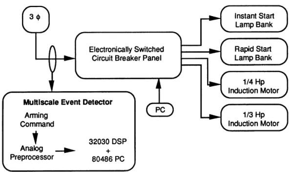
The current NILM prototype functions well with a laboratory mock-up of different loads typically encountered in commercial buildings (induction motors

and rapid- and instant-start fluorescent lamps). Figure 1.2 below shows a schematic of the laboratory platform with the NILM (Multiscale Event Detector) sampling data from three-phase power supplying a circuit-breaker panel. The laboratory-test platform requires the investigator to issue an arming command to prepare the NILM to begin the transient data acquisition and processing. Once armed, the NILM processes data continuously, searching for and matching v-sections until the algorithms are interrupted. Implementation in this manner is wasteful of computing power, because transient behavior only accounts for a small fraction of power data. In order to automate the arming step and minimize computing needs for future field tests, a pre-processing step must be developed. Researching possible algorithms for self-arming is the focus of the first part of this thesis.

Introduction 15

(16)

Figure 1.2: NILM test facility schematic. The external personal computer controls the switching on the circuit panel. Adapted from [Leeb and Kirtley, 1993]

The first objective of my research has been to develop a method to isolate a start-up (or shut-down) event and automatically sound an alarm within the

NILM to prepare it to accept a signal. Such a method of signal detection would

minimize the amount of time the NILM wastes trying to process data which have no significant meaning. The detector must be implemented as an iterative algorithm, on-line, in series with the transient identification algorithms developed by Dr. Leeb. The research discussed in Chapter 2 of this thesis is the development of an effective detector and its application to typical signals from an electric-power line.

The self-arming of the NILM is accomplished with a signal processing technique for detecting abrupt changes in dynamic systems. We propose that the logical change criterion, that signifies a turn on/off event, is a change in the steady state power signal. To a first-order approximation on/off changes in the electric load are additive to the power signal; and therefore, the signal changes we need to detect are changes in the mean power.

Change Detection Overview

A field of signal processing has grown around this need to detect changes

in time series data. In general the literature refers to 'abrupt changes in

(17)

dynamic processes.' This terminology refer to all aspects of a process' output including changes in the mean, spectral changes describing the variance and primary distribution functions of the process output. Applications for change detection are diverse, including: medicine (electrocardiograms and electroencephalograms), geology (seismic activity onset and location), manufacturing quality control (vibration or visual analysis of faults), speech recognition, etc.

There are many approaches for detecting a change in a process, and in particular changes in a signal mean. The goal for each of these approaches, though, remains constant. An ideal detection algorithm minimizes the detection delay after an event, and maximizes the average length of time between false alarms. These two criteria are strongly linked and inherently at odds with one another. Minimal detection delay implies a quick response to subtle changes in the process signal (mean, variance, distribution). Minimizing the mean time between false alarms requires relative insensitivity to subtle changes. When the signal noise is significant, relative to the size of the expected change, the trade-off between the criteria becomes critical for the design of an optimal detector.

'On-line' versus 'off-line' is a primary delineation among change detection approaches. The distinction does not imply simultaneous and non-simultaneous detection with regards to signal acquisition, but rather whether the ultimate decision made by the detector takes place within an iterative detection algorithm or within an external processor linked to a detection algorithm [Benveniste, 1986]. On-line detection examines the output of a process y(t)t2o (see, for example, the state space model described in section 1.2.3) and the conditional distribution pe[yly(t-1),....y(0)] of the output signal. This conditional distribution we recognize as a (t-1)-order Markov process, where pe[y(t)] depends on the preceding (t-1) values of y(t) and 0 is the parameter being tested (mean, variance or distribution). The goal of on-line detection is to determine whether 00 has changed to 01 at a time, r, such that the conditional probability after the change time is different from the conditional probability before the change.

peo[yly(t-1),....y(0)] * po,[yly(t-1),....y(0)] for t > r. (1.1)

(18)

Typically this determination is made with a calculated statistic g(t), with a known distribution. When g(t) exceeds a threshold value, X, the detection process stops and determines the alarm time via a stopping rule with the general form:

ta = min{t: g(t)>A] (1.2)

With on-line detection it is sufficient to observe y(t) until t=ta [Basseville and Nikiforov, 1993].

Off-line detection on the other hand is not simply a matter of recognizing ta, but also includes making judgments about 0 after the change. Off-line detection involves the testing of probability hypotheses relevant to the set of outputs y(t) where Ost N.

The null hypothesis in this procedure states that the probability of the current output's membership in a set of past outputs is equal to the distribution of all current outputs given all previous outputs.

HO: for OstsN

P{y(t) e y(t-1).} = po₀[yly(t-1),....y(0)] (1.3) The alternative hypothesis states that before a point in time, r, the probability of a certain output is distributed according to the parameter 0, and after r y(t) is distributed according to the parameter 01.

H₁: there exists r where 0srsN such that for Ostsr-1

P{y(t) e y(t-1),...} = peo[yly(t-1),...y(0)] (1.4)

and for rstsN

P{y(t) E y(t-1),....} = pe4yy(t-1),....y(0)] (1.5) The alternative hypothesis, H₁, could also be one of a set of alternative hypotheses such that we substitute for the second half of H₁to formulate a multiple model definition for the change detector [Willsky, 1986]. This situation

(19)

would arise if we know that there are a discrete number of states to which 00

can change. For n=1,...,m

Hn: there exists r where OsrsN such that for rst N

P{y(t) e y(t-1)....} = pen[yy(t-1),..y(0)]. (1.6) The off-line detector leaves the detection time, r, unknown because it is sufficient in this case to know that a particular change in 0 has occurred on the interval [0,N]. We investigate the application of off-line change detection in Chapter 3 of this thesis, and continue here with on-line detection for the arming of the NILM.

100

0 20 40 60 80

Time [min]

FIgure 1.3: Typical data acquired through end-use metering of a variable speed drive. Data acquired from monitoring of supply fan SF1 Building E19 MIT campus.

Change of Mean Detectors

For the remainder of section 1.1 we confine the discussion to on-line Change of Mean detectors where the parameter O=g. The literature [Basseville, 1986; Basseville and Nikiforov, 1993; Willsky, 1976] discusses a vast array of on-line algorithms for different applications. We mention two here

(20)

as examples. This discussion is largely drawn from the sources cited above. Consider a set of process outputs y(t) depicted in Figure 1.3 where the change to noise ratio is approximately 6:1.

Most widely used change-detection algorithms are based on a single construct, the ratio of the distribution function after the change to the distribution before the change, P0.(yY For the normal distribution

1p/ (-s)2

pe(y) = Xy- 2 (1.7)

and the ratio is typically transformed:

si = In 90 (1.8)

known as the log-likelihood ratio. Detection algorithms usually operate on a window of data from yj to yk; therefore, we define

k k

S. = si (1.9)

When the parameters 00 and 01 are known, the only unknown the on-line algorithm must find is the time of the change, tr. Optimal algorithms minimize T = ta - tr, the mean delay before detection given a fixed false alarm rate.

One of the oldest recursive algorithms for detection of a known change of mean is the Shewhart Control Chart developed in 1931 [Basseville and Nikiforov, 1993]. For a fixed sample size, N, the decision rule is given by

0 if

S1(K)<X

d

=

N and the alarm ta = {NK: d=1}. (1.10)

Equation 1.9 is repeated for K intervals of duration N until the decision rule equals one. Figure 1.4 portrays an example of how the Shewhart Control Chart is implemented with data from Figure 1.3. As the change occurs, the value of

(21)

the Shewhart Chart exceeds zero; the threshold is chosen by inspection such that extreme data will not elicit a pre-mature alarm for the change.

200 150 100 50---TesuI---50 -1 -150 -200 .

-Figure 1.4: Example of the Shewhart Control Chart with data from -Figure 1.3. In this case, N=6

and ta=NKd= 1 = 66.

Often analyses give more weight to recent observation and reduce the significance of data points which are less current. A variation of the Shewhart control charts adds a forgetting factor to the summation in equation 1.9. The decision function gk is defined

00

gk = X a(1 -X)isk-i i=0

(1.11)

where Oas1 is the forgetting factor and the alarm time

ta = min{k:gk > X}. (1.12)

These two sample algorithms serve as a starting point for developing a change detector for the NILM. These algorithms are premised on a priori knowledge of i, the mean signal after the change. Assumed availability of this information parallels the approach taken by Hart with his appliance identification algorithms for the residential NALM. The NALM assumes approximate values of (l -go) for each major residential load, and determines

(22)

the most likely turn on/off event that fits the calculated change among steady states. Hart's approach is possible for the residential setting where there is a narrowly defined range of expected loads.

For application with the commercial NILM, though, we can not assume a

priori knowledge of 1l. Diverse commercial loads can not be discretely

categorized in the same manner as residential loads. For example, induction motors vary in size from fractional horsepower to thousands of horsepower; same sized motors may have steady state loads which are an order of magnitude different from one another; and motors controlled with variable speed drives have continuously variable loads. These aspects of commercial loads make a priori estimates of 1, impossible - even with a survey of end-uses.

The expected application of the NILM also discourages on site surveys which might be considered intrusive or infeasible because of the inaccessible location of many end-uses.

We conclude that the presented change detectors are inappropriate for the

NILM application. We develop a change of mean detector for the NILM in

Chapter 2.

1.2 Application 2: Fault Detection and Diagnosis

Chapter 2 of this thesis develops of on-line change of mean detection algorithm appropriate for the non-intrusive load monitor. Chapter 3 discusses the use of this same algorithm implemented off-line to interpret an induced change in an output signal. Instead of using the change of mean detector to merely locate important data from a continuous stream of information, we will use the output from the algorithm to evaluate the system that generates the output.

Relevance of Fault Detection and Diagnosis

Fault detection and diagnosis (FDD) in HVAC systems is a growing issue in the realm of HVAC system design and operation. The driving forces behind this interest are both need and ability based. There is a perceived need for FDD in building thermal systems for energy conservation, better indoor comfort and climate control, and to facilitate better systems operation to counter increasing system complexity which may be outpacing the skills of system operators. Off-setting the increased complexity of HVAC systems are advances

(23)

in our ability to thoroughly monitor operating systems with desktop computers. These computers allow us to cheaply process the wealth of data generated by monitoring, and present useful information about a system's condition to the system manager. With current information processing technology it is possible to implement effective FDD at moderate cost.

Since the oil price shocks of the 1970s building managers have become more concerned with the energy consumption in buildings. Concerns about unstable and high energy prices have prompted the widespread use of building energy management systems (BEMS) in commercial facilities. A BEMS utilizes computers to control the energy systems to minimize the energy use and energy costs in the building. A BEMS does this by using outdoor air to a greater extent and extensively scheduling and prioritizing the operation of HVAC equipment to minimize utility demand charges and peak use rates. Central control of the building energy systems with a BEMS allows a building operator to coordinate all of the diverse components of the system and avoid contradictory control schemes.

To gain the full benefit of a BEMS, HVAC systems need more complex equipment (economizers, variable speed drives) and further instrumentation for coordinated control of these devices. Though modern equipment is more reliable than in the past, the number of components which can fail has increased and their configuration makes it difficult to locate the problem once a fault has occurred. Failure to notice a fault or locate it quickly once it is detected can greatly increase the operation and maintenance costs of the HVAC system.

By integrating a FDD regime within a building operating system, FDD could

assist the building operator and reduce costs.

Goals of FDD

Faults within a building's HVAC system are classified into two general categories: those which are a result of abrupt component failure and those which develop over time as a result of slow deterioration of performance. Examples of abrupt failures would be the mechanical breakdown of a fan or pump motor or a cut wire from a sensor. Deterioration faults would include a gradual drift in a sensor's calibration or slow clogging of a heat exchanger. A single fault of either type does not necessarily cause immediate system-wide failure or even a failure to maintain indoor comfort. In most faulted HVAC

(24)

systems the automatic control regimen will take compensatory action to maintain the necessary set points. For example, to compensate for a heat exchanger with a diminished heat transfer coefficient from scale deposits on the water side, the controller will simply demand more water flow through the coils such that the temperature gradient between the water and air sides offsets the effects of the scaling. Only when scaling is so severe that a sufficient gradient can not be maintained will the building occupants notice a change in the comfort level.

Though a fault's effect on indoor comfort may not be immediately apparent to the occupant, the rest of the system does bear the burden of the fault. For example, we consider an improperly tuned controller for a heat exchanger valve. If the gain is set too high, the controller will overshoot the steady-state position and possibly oscillate unnecessarily. Repeated direction reversals and excessive travel will wear the valve and actuator prematurely, resulting in failure of these components. Early detection of the initial fault is critical for avoiding secondary failures which can cascade throughout a system leading to costly

maintenance.

Analogous with the trade-offs inherent with the design of change detectors, an FDD system must trade-off the benefit of finding a fault quickly with the possibility of falsely identifying a fault and incurring excessive maintenance costs investigating false alarms. The goal of FDD should be to identify the fault before it causes further failures within the system, while minimizing the number of false alarms. If HVAC faults are generally degradation-type, a long delay before detection is appropriate while the detector accumulates sufficient information to indicate with great certainty that a fault exists. Conversely, catastrophic faults need to be detected rapidly before failure spreads through a

system.

In addition to the cost of false alarms and missed detection, FDD design must consider the costs of implementation. The cost of extra sensors for monitors and computers for data processing must not exceed the expected benefit derived from the fault detector.

Approaches to FDD

All approaches to fault detection and diagnosis have some aspects in

common, because of their common goal - finding differences between

(25)

established normal operation and actual operation which indicate failure. The procedure of FDD generally includes three steps: residual generation, data processing, and classification.

Residuals are the computed differences in the system state between actual operation and expected fault-free operation. The magnitude of the residual often correlates with the severity of the failure (eg. r =T(actual)

-T(expected) [Salsbury, eta., 1994]).

Data processing is used to convert residuals into values, or 'innovations', which have known statistical properties. This step is essential for filtering out noise or aberrant data points. A common innovation is the normalized squared residual (rn2 ₌

()2 ) [Usoro, et al.,

1984].

The final step, classification, makes logical (if-then) judgments about the innovation. Is the innovation large enough to imply a fault in the system? What are the residuals from other variables and what combination of these residuals implicates a specific fault in a specific location?

Various FDD methodologies address these steps with different efficacy depending on the type of fault the method is designed to detect. Some approaches are more quantitative, other methods utilize greater degrees of abstraction. In this discussion we will look at three different fault detection methodologies: 'landmark states', 'physical modeling' and 'black-box modeling.' The close similarities among the techniques is very apparent. These three methods are by no means exhaustive of the FDD field. Fuzzy logic

[Dexter and Hepworth, 1994; Dexter and Benouartes, 1995], artificial neural networks [Dubuisson and Vaezi-Nejad, 1995; Li, et a/., 1994] and other approaches are all being actively investigated.

Landmark States

The first method discussed here is based on 'landmark states' of an operating system. The theory behind this method is that an HVAC system will 25 Introduction

(26)

operate in a given mode or state depending on specific monitored variables. The landmarks at which the system is analyzed are "physical values which have special significance, such as freezing and boiling" [Glass, 1994], ambient conditions or a scheduled time. A very basic example of this method would be the detection of a fault in a fan motor on-off switch. If the motor is supposed to

switch off at the end of the occupancy period, the system could detect a failure

by examining one of many variables which might be monitored during normal

operations such as: static pressure in the duct, motor shaft rotational velocity or power consumption.

Glass [1994] presents a more sophisticated application of this method to determine whether a system's controller regimen is functioning properly. His research examines the operation of a central air handling plant which consists of heating and cooling coils and air dampers to control the mix of outside air

(TOA) and return air (TR). Given the qualitative relationship between these two

temperatures, he derives the following table to determine the proper operating mode of the air handling plant.

Table 1.1 - Operating regimes of a central air handling plant [Glass, 1994] Temperature Qualitative Temperature Controller State

relationship relationsips

TOA TR TOA comparatively low Dampers set for minimal outside air and the heating coil operates. TOA TR Tmix= Tsupply within Heating and cooling coils switched

operating range of the off and the controller operates the

bypass dampers dampers in the normal mode.

TOA TR TOA comparatively high Dampers set for maximal outside air and the cooling coil operates.

TOA > TR TOA comparatively low Dampers set for maximal outside air and the heating coil operates.

TOA > TR Tmix= Tsupply within Heating and cooling coils switched operating range of the off and the controller operates the

bypass dampers dampers in the normal mode.

TOA > TR TOA comparatively high Dampers set for minimal outside air I and the cooling coil operates.

(27)

The transitions among the quantitative and qualitative temperature relationships constitute the landmark states for fault detection. Information about the return and outdoor air temperatures determines the controller state which can be confirmed with the control signals. Discrepancies between these two sources indicate the presence of a fault. For this application this methodology is very straightforward with very little computation and relatively simple classification rules for faults. To expand the method to include more types of faults would require additional instrumentation for acquiring data and more classification rules to relate operating states to the monitored data. To successfully implement a FDD scheme, which is general enough to detect a wide range of faults, it would be necessary to develop detailed operating rules for many permutations of operating conditions for each system component.

Physical Models

A second method of FDD is commonly known as 'physical modeling' which

directly or indirectly compares data from established correct operation of a system with faulty operation. Simultaneous comparison of many variables, called residual generation above, is used to classify the exact nature and

location of the fault. Most FDD research with this method employs computer simulations of the HVAC system to be studied. An actual operating system can be used to study this FDD method, however computer simulations are preferred for research because it is easier to control the simulation of faults on a computer.

These models are based on physical engineering relationships and typically simulate a period of operation during which various perturbations are introduced into the system such as changes in the outdoor air temperature or changes to the supply air temperature set point. Several system variables (pressures, temperatures, flows, power....) are monitored simultaneously during the simulation. The changes in these variables due to the perturbations are noted and recorded. Simulated faults are then introduced into the model and it is run again with the same set of perturbations.

The output data from the simulation runs are then processed to remove signal noise. Residuals, the differences between output collected during correct operation and faulty operation, are calculated for all time intervals in the 27 Introduction

(28)

simulation. If we exclude the feedback information into the model, Figure 1.5 shows the schematic for residual generation with physical models. Feedback control of the plant itself is implicit. The magnitudes of the residuals depend on the variables measured; therefore, they are typically transformed into dimensionless variables. The set of dimensionless residuals is then used to develop fault rules which uniquely identify and characterize a particular fault. In

most cases of FDD the fault classification is based on steady-state system operation.

Dumitru and Marchio [1994] present a typical example of this method. With the building simulation tool, DOE2, they modeled a single zone constant air volume fan system. By comparing hourly output data from a simulation of the fault-free, reference configuration to comparable data from model runs with faults, they established conditions of faulty operation which can be determined

by monitoring selected variables. For example, they studied the behavior of

their HVAC system model when they assumed the outside air damper was stuck in the full open position. On a warm humid day which requires air conditioning, this failure can be identified by an increased mixed (outside and return) air temperature, increased mixed air humidity ratio and increased energy transfer to the cooling coil in order to maintain the supply air temperature, relative to the fault free simulation. For this example with this methodology, the deviation from the reference system which is most difficult to discern is the mixed air temperature. In this case a difference of 30_{C in the mixed air is required to}

uniquely define this fault.

Differences among applications of this method usually involve monitoring different variables depending on the type of fault which is targeted in the research and different residual processing to arrive at unique innovations which adeptly characterize a fault. Physical modeling has many significant advantages when compared to other methods. Among these is the direct representation of the components of the system with standard engineering equations. The equations simplify the process of extracting physical parameters such as flows and heat transfer coefficients which often exhibit changes during faulty operation. Physical models implemented on a computer allow the investigator to monitor many variables simultaneously with little additional cost (increased simulation time).

(29)

Well constructed physical models of HVAC systems are also considered accurate for the full operating range of the system [Fargus, 1994]. This factor is important for fault simulation because the range of faults encountered in HVAC systems does not fit neatly into discrete definitions. In the example presented above, the damper was stuck full open. It is probable, though, the damper would fail in an intermediate position; therefore, the ability to interpolate and extrapolate conditions of failure is critical for a truly comprehensive fault detection and diagnosis regimen.

The significant disadvantage of physical models is their extensive computation needs for processing data generated with a computer simulation or data collected from a real system. Computer simulations have the added disadvantage of complex formulation. A typical HVAC system involves many variables and simultaneous processes. Constructing a model, whether static for steady-state modeling or dynamic, is very demanding. Problems with numerical instability for dynamic models can become paramount.

Black-Box Models

The third general method of fault detection employs 'black-box' models. These are mathematical models which relate input characteristics of a system to known outputs. Implicit in black-box modeling is knowledge of how the HVAC system should function given a set of inputs. Black-box models are developed from data collected from operating real systems or physical models such as those previously described. These operating data are used to 'train' the black-box model to arrive at the known outputs given relevant inputs to the model. Figure 1.5 below is a schematic of how black box models are implemented with an operating HVAC plant. Fault detection with these models is a matter of either interpreting changes in the residual, r, or interpreting changes in the parameters of K which are fed back into the model to minimize r.

Introduction 2929

(30)

Figure 1.5: Schematic of a Black-Box model with inputs, u; outputs, y; disturbances and faults

d and f, respectively; residuals r and model parameters K Figure adapted from [Sprecher, 1995].

Black-box models use a combination of weighted linear and non-linear functions (polynomials or splines, for example) to optimally map inputs to outputs, minimizing error. These functions may or may not have direct physical meaning in the sense of engineering concepts such as energy balance equations or individual parameters such as heat transfer coefficients. In the absence of direct representation of these engineering criteria, additional computation is required to extract this information when it is necessary.

The accuracy of a black-box model is directly related to the amount of data used to train the model and the range of operating conditions from which the data was collected. Research has shown that these models are extremely reliable when they are interpolating between operating points used to train the model, but reliability diminishes rapidly when the model needs to extrapolate beyond its training range [Fargus, 1994]. This limitation is especially troublesome in a real application if the training data is collected before the building is fully occupied because the presence of occupants will affect the

model parameters.

Despite these disadvantages, black-box models are increasingly common in FDD research for several reasons. The derivation of the model parameters is computationally easier than solving for the state variables in a physical model; therefore, once the model is trained implementation of the fault detector is easier. They are generally accepted to provide reasonable approximations to actual systems, and different techniques to counter problems of data scarcity

(31)

within the operating range of the training data, such as neural nets and fuzzy logic, are rapidly becoming more common [Dexter and Hepworth, 1994; Fargus, 1994].

An example of a black-box model is based on concepts from modern control theory, state space analysis and the Kalman filter. This discussion is based on research done by Usoro et al [1984] Typical state space equations look like 1.1 3a and 1.1 3b below.

* = f(x,u,z,r) y = h(x,u,z,w) 0 = g(x,u,z) (1.13a) (1.13b) (1.1 3c) Where:

x = a state vector of the dynamic components of the system: actuators, controllers and heat exchangers.

f = a vector of non-linear functions

u = a vector of controller set points and external inputs outdoor air, or hot and chilled water temperatures

z = a vector of parameters such as pressures and flows r = zero-mean, gaussian, process noise

y = a vector of sensor outputs

h = a vector of non-linear functions

w = zero-mean, gaussian, sensor noise

g = a vector of non-linear algebraic functions

sensors,

such as

Equation 1.13c represents a set of simultaneous algebraic equations which typically are not a part of standard state space problems. If these equations are solved for z and substituted into Equations 1.13a and 1.13b the state space equations take their standard form.

For a computer simulation these equation are transformed into discrete state space equations with the process and sensor noise occurring additively and linearly.

x(k) = f(x(k),u(k),z,k) + r(k)

y(ki) = h(x(k),z,ki) + w(ki)

(1.14a) (1.14b)

(32)

where ki is an index of the sampling time.

The estimate of the state vector in the next time step given the state in the present step is

x(klki1) = x(ki.1Iki.1) + t f(x(k),u(k),z,k) dk. (1.15)

k-1

and x(kilki) = x(kiki.1) + K(ki)[y(ki) - h(x(kilki.1),z,k)] (1.16) where x(kolko) = xO, the vector of initial conditions, and K(ki) is the gain matrix defined:

K(ki) - k I (kilki.₁) HT(kijki-1) (1.17)

~H (kilki.1)E,(kilki.1)HT(kilki.1) + W'

In the gain matrix, K, X(alb) is the state covariance matrix between points a and b. H is the first order linear approximation of h, at the point x(kilki.1), and W is the sensor noise covariance matrix which, when the noise is zero-mean and gaussian, equals 0.

H =

(i+hA

+ ₁ 22 + ....) when A is the sampling time interval

l(kijki.1) = (ki.1|ki)X(ki.1ki.1i)DT(ki.1|ki) + R (1.18)

X(kilki) = [ I - K(ki)H(kilki-₁₎X(kilki.1)] (1.19)

<D is the state transition matrix corresponding to the linear approximation of

f, along the trajectory x(kilki.1) kl.15 k<ki, and R is the process noise covariance

matrix which, like the sensor noise, equals 0.

This is sufficient information to solve Equation 1.16 for the term in the brackets which is the residual or the difference between the observed vector y and the modeled approximation of y.

a(ki) = y(ki) - h(x(kilki.1),z,ki). (1.20)

Under fault free operation a should be zero-mean and gaussian.

32 Chapter 1

(33)

Alternatively, if we are not interested in the state variables, equations 1.1 4a and 1.14b can be written as follows

x(k+1) = Ax(k) + Bu(k) + r(k) (1.21a)

y(k) = Cx(k) + w(k) (1.21b)

which, when x and z are neglected, are simplified to

y(k) = Mu(k) + v(k). (1.22)

This is the formulation of a straightforward auto regressive moving average model with exogenous inputs (ARMAX), u and outputs, y. The vector, v, is the linearly combined process and sensor noise, and M is a new parameter matrix consisting of the gains for each components of the system. Faults will manifest themselves as residuals in the elements of M [van Duyvenvoorde, et aL, 1994;

Yoshida and Iwami, 1994].

FDD Techniques Summary

In summary, the three presented fault detection and diagnosis techniques share many points. Each method generates a residual which we call the fault detection step. In the case of landmark states, that residual is simply a'yes' or a 'no' answer to the question is the controller regime consistent with the observed temperatures. Residuals for the physical and black-box models are the differences between observed and expected outputs or parameters.

The data processing for the techniques also differs among the three examples. The landmark states method bypasses this stage because there is no quantitative data to analyze. The physical model generates outputs which must be made dimensionless with known distribution and the Kalman filter implicitly derives a zero-mean gaussian parameter, i, when the system operates correctly.

The final FDD step is fault diagnosis which is the classification of residuals. Classification is based on a set of conditional rules which must be satisfied to determine the nature of the detected fault. These rules are specific to the the methodology and the type of fault observed. The rules are derived by testing the model in many varying degrees of faulty operation to determine at what

Introduction 3333

(34)

point the innovation indicates faulty operation as distinct from correct operation. This step is not explicitly described here, because of its case specific nature.

Chapter 3 of this thesis develops a fault detection and diagnosis methodology structured around the change of mean detector investigated in Chapter 2.

34 Chapter 1

(35)

Chapter

2 CHANGE

of

MEAN DETECTION

In the introductory Section 1.1, we discussed the need for a signal processing tool capable of detecting changes in the mean output signal from of system. Such a tool is necessary for self-arming an advanced electricity

monitor, the non-intrusive load monitor (NILM). We cited two examples of change detectors often used, but stated that they were inappropriate for application with the NILM because knowledge of the signal mean after the change is needed. This chapter develops an appropriate algorithm and tests it with electric power data collected from metered sources on the MIT campus. First we examine the change detection algorithm used by Dr. Hart for the

residential NALM.

2.1 Residential Power Change Detection

Integral to the NALM are algorithms which identify changes in the steady state power level. Hart's change detection algorithm is straight forward and effective for residential loads which are dominated by steady, resistive and finite-state (on/off) loads. The essence of the algorithm is a single-pass, average steady power comparison. We demonstrate its use below with commercial electric load data.

The NALM algorithm segments the power data into periods of steady power and changing power. Steady power is defined by a string of at least N consecutive data points that fall within a pre-determined bandwidth about an average power level. Periods of changing power are all data that are not steady. Transition begins when the first time-series datum falls outside of the power bandwidth. Transition ends when the next N consecutive points fall within the bandwidth about a new, unknown average power level. The data 35

(36)

during each steady period are averaged to minimize the effects of noise, and the change between average power levels is used to determine which appliance has turned on or off. The tuning parameters for the NALM change-detection algorithm are the size of the bandwidth about the mean power level and the number of data needed to define steady state. For its residential application these parameters were ±15W and 3 samples, respectively [Hart,

1992].

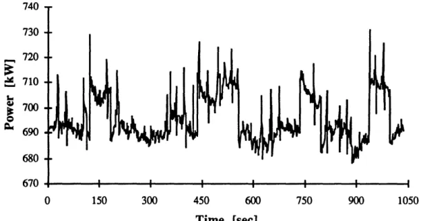
Figure 2.0a on the following page presents one-second averaged data measured at the electric service entrance for HVAC equipment in a commercial facility. It is possible to visually identify four events lasting approximately 60, 120, 60, and 60 seconds, respectively. At these times a condensed water pump is switched on and off [Norford, et al., 1992]. The underlying power level includes the rest of the HVAC equipment and general process and sensor noise. Clearly, the parameters used for the residential application of the NALM would be inappropriate for commercial load monitoring.

Assuming the data set in Figure 2.0a is representative of commercial loads, we test combinations of the tuning parameters to determine the potential for applying the residential NALM change-detection algorithm with the commercial NILM. Figures 2.Ob through 2.Og display the results of these experiments with the NALM change-detection algorithm, and Table 2.0 summarizes the significant aspects of the figures for determining their appropriateness. The significant features in these figures are the transitions from 100 to zero. At these points the preceding steady period ends and the algorithm begins searching for the next portion of steady data. The 'ideal' implementation of the the NALM algorithm would be a line at 100, interrupted by only eight brief transitions to zero at the designated change times. We display results where ten and twenty consecutive data points determine steady state, and where the bandwidth is ±2, 3 and 5 standard deviations from the mean power level (respectively, ±3.4, 5.1 and 8.5 kW).

(37)

740 730 720 710 700 690 680 670 150 300 450 600 750 900 Time [sec]

Figure 2.0a: One-second average power data logged at the electric service entrance to a

commercial HVAC room. Four turn on/off pairs [-130,190], [-440,560], [-730,790], and

[-940,1000] are the features of note among a noisy environment [Norford, et al., 1992].

a 100--A oa 0 0 150 300 450 600 750 900 1050 Time [sec] 100 0 150 300 450 600 750 900 Time [sec]

Figures 2.Ob and 2.0c: Hart steady state detector: threshold bandwidth = 2- = ±3.4 kW; ten

and twenty consecutive points, respectively, within the bandwidth determine steady state. Points at zero imply the power levels are in transition.

Change of Mean Detection 37

1050

(38)

740 730 720 710 700 690 680 r 670 t 0 150 300 450 600 750 900 Time [sec] Figure 2.0a: Repeated for ease of comparison.

100 0 150 300 450 600 750 900 Time [sec] 100 0 0 150 300 450 600 750 900 Time [sec]

Figures 2.Od and 2.0e: Hart steady state detector threshold bandwidth 3a-=±5.1 = kW; ten

and twenty consecutive points, respectively, within the bandwidth determine steady state. Points at zero imply the power levels are in transition.

1050

(39)

740 730 720 710 700 690 680 '' '" 670 I I I I i 0 150 300 450 600 750 900 Time [sec] Figure 2.0a: Repeated for ease of comparison.

100 0 100 0 150 300 450 600 750 900 Time [sec] 0 150 300 450 600 750 900 Time [sec] Figure 2.O and 2.0g: Hart steady state

and twenty consecutive points, respectively, at zero imply the power levels are in transition.

detector threshold bandwidth 5- = ±8.5 kW; ten

vithin the bandwidth determine steady state. Points

Change of Mean Detection 39

1050

(40)

Table 2.0: Steady State Detector Efficacy

Time in Significant Transition Transition Events

Figure BW [kW N Periods I% Detected

2.Ob ±3.4 10 47 37 6/8 2.Oc ±3.4 20 14 74 1/8 2.Od ±5.1 10 39 22 6/8 2.Oe ±5.1 20 19 45 2/8 2.Of ±8.5 10 32 11 7/8 2.0g ±8.5 20 18 28 2/8

Unfortunately, we find the residential-NALM change detector unsatisfactory for this data set. Definitions of steady state power made with small N are too unstable, thus the alarm sounds frequently for insignificant changes in the signal. As we address later, low false alarm rates are crucial for the NILM application. Steady state definitions with large values of N tend to miss significant events because the algorithm is unable to find steady regions in the signal because N is too inclusive.

Data presented here show a maximum bandwidth about the average signal of ±8.5 kW. The minimum significant change is approximately 18 kW; however, spurious pulses typically exceed 20 kW. Relaxing the bandwidth reduces false alarms somewhat , though they still occur, and the danger of missing smaller significant events increases. In general, this change detector is extremely sensitive to signal noise, and it has difficulty finding steady regions because of continuously varying loads.

2.2 Change Detection Necessities

Before we begin our search for an appropriate change of mean algorithm we define the task more precisely, in terms of optimality criteria for the detector and the character of power use signals. From the perspective of the NILM, the change of mean algorithm must meet three loosely defined criteria. First, the algorithm must have a low false alarm rate because the computational expense of unnecessary v-section matching must be avoided. Implicitly this means that the algorithm must be insensitive to signal noise. Second, the algorithm must be rapid, requiring minimal operations at each step. If the frequency of

(41)

monitored turn on/off events is high, thus requiring the majority of the processing time for transient identification, easy calculation for the change detector might become paramount. Finally, delay before detection should be small, though not at the expense of the false alarm rate. All of the power signal data acquired by the NILM passes through a temporary storage buffer, so that no necessary information will be lost, if v-section determination and identification is needed. The current prototype NILM begins its transient identification procedure with thirty pre-transient points. Allocating memory for a few more points in this segment of data would be the price for longer detection delay.

The next step in our pursuit of an appropriate change detector is to investigate the properties of the power signal that the NILM examines. The power transients, that the NILM isolates and identifies, span a broad range of time frames. Some power factor correction transients last tenths or hundredths of one second. The fractional horsepower motors tested in the laboratory mock-up have transients which last a comock-uple seconds (see Figure 1.1), larger induction motors in HVAC systems have transients which might last tens of seconds, and finally 'soft-start' features with variable speed drives can attenuate the start-up transient by ramping the motor up to full speed over several minutes. Depending on the sampling rate, these different length transients either look like significant signal, noise or signal drift.

In general, power data are extremely variable. Data in Figure 2.Oa

[Norford, et al., 1992] indicates that the NILM should expect significant noise in the power signal of HVAC equipment. One-minute average data presented below is similarly awash with noise. When attached to the utility service entrance to the building the signal sampled with the NILM will certainly confront significant noise because process variance for each end-use is additive to the first approximation.

The signal changes the detector must isolate span a broad range of magnitudes. In practice, the NILM might only be used to monitor large commercial loads (similar to the NALM which only identifies large residential loads). However, these loads will vary significantly within a facility and among facilities. It is reasonable to assume the range will include two or three orders of

magnitude with an unknown distribution within that range. Adding to the issue of the signal magnitude is the fact that transient amplitude (which can be an

(42)

order of magnitude greater than steady state) correlates not only to the size (rated, steady state power) of the end-use, but also the type of end-use (Figure

1.1). And finally, the magnitude of a given transient can vary relative to the

instant during a standard 60 Hz cycle when the load is turned on [Leeb, 1993]. Taken together, the points listed above make change of mean detection for the NILM a difficult task.

2.3 Known versus Unknown 01

All change detectors are developed with some a priori knowledge or

assumptions about the data that must be analyzed. In many cases this knowledge includes information about the expected magnitude of the change, v

= 101 -00|. The information can be extremely specific, 01 is deterministic, or less precise, such as knowing the distribution of 01 or even only the most likely value of 01. Different levels of a priori knowledge affect the choice of detection algorithms and their optimal configuration.

The detection algorithms presented in Section 1.1 assumed deterministic information about