HAL Id: hal-01331722
https://hal.archives-ouvertes.fr/hal-01331722
Submitted on 14 Jun 2016HAL is a multi-disciplinary open access
archive for the deposit and dissemination of sci-entific research documents, whether they are pub-lished or not. The documents may come from teaching and research institutions in France or abroad, or from public or private research centers.
L’archive ouverte pluridisciplinaire HAL, est destinée au dépôt et à la diffusion de documents scientifiques de niveau recherche, publiés ou non, émanant des établissements d’enseignement et de recherche français ou étrangers, des laboratoires publics ou privés.
Non-linear simulation of coiling accounting for roughness
of contacts and multiplicative elastic-plastic behavior
Daniel Weisz-Patrault, Alain Ehrlacher, Nicolas Legrand
To cite this version:
Daniel Weisz-Patrault, Alain Ehrlacher, Nicolas Legrand. Non-linear simulation of coiling accounting for roughness of contacts and multiplicative elastic-plastic behavior. International Journal of Solids and Structures, Elsevier, 2016, 94-95, pp.1-20. �10.1016/j.ijsolstr.2016.05.012�. �hal-01331722�
Non-linear simulation of coiling accounting for roughness of
contacts and multiplicative elastic-plastic behavior
Daniel Weisz-Patraulta, Alain Ehrlacherb, Nicolas Legrandc aLMS, ´Ecole Polytechnique, CNRS, Universit Paris-Saclay, 91128 Palaiseau, France.
bLaboratoire Navier, CNRS, ´Ecole Ponts ParisTech, 6 & 8 Ave Blaise Pascal, 77455 Marne La Vallee, France cArcelorMittal Global Research & Development East Chicago 3001 East Columbus Drive, East Chicago, IN
46312, USA
Abstract
In this paper numerical simulations of coiling (winding of a steel strip on itself) and uncoiling are developed. Initial residual stress field is taken into account as well as roughness of contacts and elastic-plastic behavior at finite strains, considering the Tresca yield function and isotropic hardening. The main output is the residual stress field due to plastic deformations during the process. This enables to quantify additional flatness defects. The presented coiling simulation relies on a modeling strategy that consists in dividing each time step into two sub-steps. Each sub-step can be solved semi-analytically and numerical optimizations enable to obtain a gen-eral solution. Thus reasonable computation times are reached and parametric studies can be performed in order to develop coiling strategies considering the process parameters. Compar-isons with previous models from the literature are presented. Moreover the comparison with a Finite Element simulation presents the same order of magnitude, however it shows that direct computations using classical FE codes are difficult to perform in terms of computation times and stability if an explicit integration scheme is chosen. Numerical results are also given in order to determine the effect of some parameters such as roughness, yield stress, applied force, strip crown or mandrel’s radius.
Keywords: Coiling, Roughness, Contact, Multiplicative elasto-plasticity, Finite strains, Optimization
Ω0 Semi-infinite domain
S0 Cross section
eX, eY, eZ Cartesian basis
X, Y, Z Cartesian coordinates (reference configuration) δ(Z) Strip geometrical profile through thickness
L Strip half-width
tc Strip thickness at the center
te Strip thickness at the edges
Rext
mand External mandrel radius
Rint
mand Internal mandrel radius
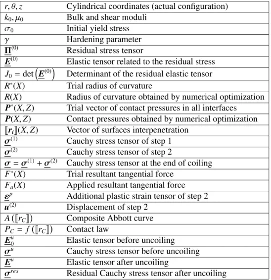
r, θ, z Cylindrical coordinates (actual configuration) k0, µ0 Bulk and shear moduli
σ0 Initial yield stress
γ Hardening parameter
Π(0)
Residual stress tensor
E(0) Elastic tensor related to the residual stress J0 = det
(
E(0)) Determinant of the residual elastic tensor R∗(X) Trial radius of curvature
R(X) Radius of curvature obtained by numerical optimization P∗(X, Z) Trial vector of contact pressures in all interfaces
P(X, Z) Contact pressures obtained by numerical optimization JriK(X, Z) Vector of surfaces interpenetration
σ(1) Cauchy stress tensor of step 1
σ(2) Cauchy stress tensor of step 2
σ = σ(1)+ σ(2) Cauchy stress tensor at the end of coiling
F∗(X) Trial resultant tangential force Fa(X) Applied resultant tangential force
εp Additional plastic strain tensor of step 2
u(2) Displacement of step 2
A(JrCK
)
Composite Abbott curve PC = f (JrCK) Contact law
Eu0 Elastic tensor before uncoiling σu Cauchy stress tensor before uncoiling
Eu Elastic tensor after uncoiling
σres Residual Cauchy stress tensor after uncoiling
Table 1: Nomenclature
1. Introduction
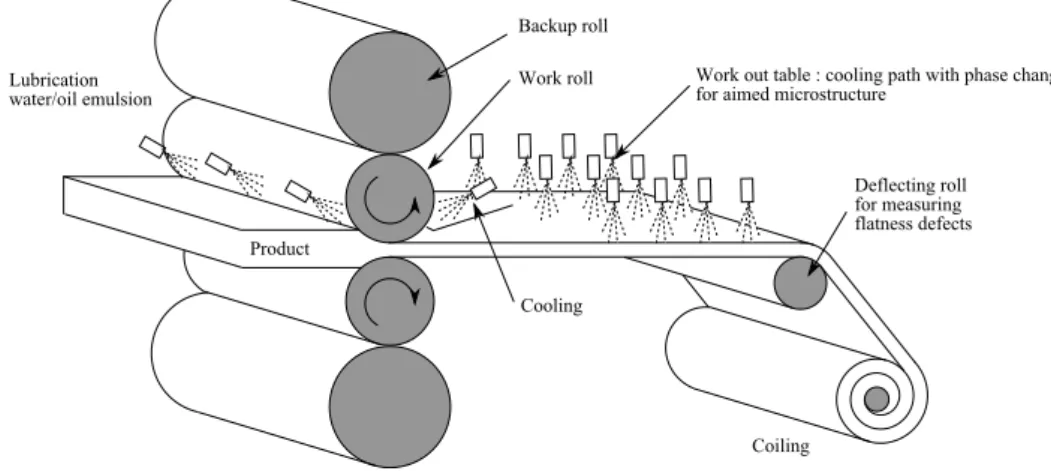
The coiling process consists in winding under tension a steel strip on a cylindrical man-drel. This process is very commonly used for storage in the steel-making industry and takes place after two main processes namely the rolling process on the one hand where the strip thickness is reduced between two rotating rolls and the run out table on the other hand where a cooling path is imposed in order to reach a targeted micro-structure. A schematic view of these is presented in figure 1. Large heterogeneous plastic deformations and phase changes occur during these latter processes leading to significant residual stress issues. Residual stress profiles are called flatness defects because they are responsible for out of plane deformations when tension is released and the strip is cut. Flatness prediction is one of the major issue of the steel-making industry, thus many papers proposed numerical simulations of rolling pro-cess in order to improve knowledge of residual stresses as a function of rolling parameters. One can mention a review of numerical simulations of rolling process published by Montmi-tonnet (2006). Jiang and Tieu (2001) proposed a rigid plastic/visco-plastic FEM and Hacquin (1996) published a 3D thermo-mechanical strip/roll stack coupled model called LAM3/TEC3 developed by Cemef, Transvalor, ArcelorMittal Research and Alcan. Abdelkhalek et al. (2011) computed the post-bite buckling of the strip, which is added to the older simulation of Hacquin
(1996). Nakhoul et al. (2014) used a coupled Finite Element Modeling in order to predict man-ifested flatness defects. The impact on flatness of heterogeneous temperature field on the one hand and friction on the other hand is investigated. Kpogan and Potier-Ferry (2014) developed a simplified numerical method in order to predict the response of long thin strips considering residual stresses. Nakhoul et al. (2015) developed a two-scaled buckling model to predict the occurrence and geometric characteristics of manifested flatness defects. Recently Cuong et al. (2015) published an experimental and numerical modeling of flatness defects. Furthermore inverse methods dedicated to experimental evaluation of contact conditions during the rolling process have been developed in order to offer an experimental counter-part to predictive models. For instance, Weisz-Patrault (2015) reviewed some flatness control procedures and proposed an inverse Cauchy method using conformal mapping techniques that evaluate the residual stress profile in the strip. In addition, Weisz-Patrault et al. (2011, 2013b) published fast inverse meth-ods (in 2D and 3D) dedicated to contact stress evaluation in the roll gap in real time during the rolling process. An experimental study based on this inverse method and optical fiber mea-surements has also been proposed by Weisz-Patrault et al. (2015b). Fast inverse methods have been developed for the thermal characterization of the contact between the strip and the work roll during the rolling process in 2D and 3D by Weisz-Patrault et al. (2012a); Legrand et al. (2013) and a thermo-elastic coupling have been published by Weisz-Patrault et al. (2013a). Experimental studies showing the feasibility of temperature measurements during the rolling process and performances of the associated inverse methods have been led by Weisz-Patrault et al. (2012b); Legrand et al. (2012); Weisz-Patrault et al. (2014).
Figure 1: Schematic view
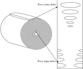
Specific flatness defects occur during the coiling process as illustrated by Counhaye (2000). Indeed, for rather thick strips or small mandrels radii the curvature can generate significant plas-tic deformations. Furthermore, the geometrical strip profile of a cross section is not rectangular but more often parabolic, thus the strip center is thicker than the edges. Therefore the contact of the strip on itself is not ensured all along the coil width and a barrel shape is commonly ob-served. Usually the contact length decreases from the first layer to the last one and concentrates at the strip center (for parabolic geometrical profiles where the strip center is thicker). Conse-quently the contact pressure increases. This induces over-tension in the strip that is responsible for plastic deformations especially for the last layers where long center defects (or wavy center) are often observed because plastic elongations are localized at the center. Moreover when large
coils are obtained the first layers near the mandrel are submitted to large compressions that can also induce plastic deformations and short center defects (or wavy edges) are observed because plastic shrinkage is localized at the center. These defects are presented in figure 2. In addition, when the coil cools down phase changes occur modifying the residual stress distribution. Thus, modeling the coiling process is part of the general effort to predict flatness defects. There are several attempts to simulate effectively the winding of a strip on a mandrel.
Figure 2: Specific flatness defect
Edwards and Boulton (2001) presented major issues related to the coiling process as well as an interesting review of the early models. For instance, soft or tight center collapses of coils are described on the basis of industrial experiences, however the present contribution does not deal with such issues and focuses on numerical coil winding simulation. Most of coil winding models use thin or thick-walled elastic theory for hollow cylinders. Within this frame work Sims and Place (1953) proposed an approach based on the theory of wire-winding of gun barrels. Based on experimental results, Wilkening (1965) emphasized that the model proposed by Sims and Place (1953) fails after 55 wound wraps, because stresses are widely overestimated. Altmann (1968) introduced an analytical solution considering constant radial Young’s modulus, but tangential stress could not evolve. Wadsley and Edwards (1977) fixed the radial Young’s modulus of the coil to a very low value compared with the standard value of the constituting material. This anisotropy is an attempt to model roughness of contacts. Thus, the coil is modeled as a hollow cylinder but the radial Young’s modulus is decreased in order to take into account surfaces interpenetration due to roughness. However the strip thickness variations are not taken into account. The model proposed by Edwards and Boulton (2001) also uses a radial Young’s modulus that varies with the number of wound wraps. However it seems that contact is imposed all along the coil width, no open gaps are formed between the wraps at any point. As detailed above, the contact length actually decreases because of the geometrical profile of the strip. It is considered that results in zones where the contact is e ffec-tively ensured are not very affected by the assumption consisting in imposing contact all along the strip width. Hudzia et al. (1994) also developed a model (for which radial anisotropy has been added later) that takes into account the contact length evolution during the coil winding. However, the mid-plane radius is not inferred from the elastic non-linear problem but imposed
a priori. Kedl (1992) proposed a model where wound wraps are computed as thick-walled cylinders on top of one another. The radial Young’s modulus is set as a function of contact pressure in order to model roughness. Lee and Wickert (2002) proposed a two-dimensional Finite Element analysis. ¨Ar¨ol¨a and von Hertzen (2007) developed a Finite Element model in a total Lagrangian formulation. An hyperelastic, anisotropic and radially non-linear behavior is considered. Axial and radial displacements are accounted for. One can also mention the work of de Hoog et al. (2007) which consists in fixing the resulting stress in the coil and inferring by inverse method the winding tension profile. This study is based on hyperelastic non-linear material. Liu (2009) published a non-linear elastic model based on displacement formulation that takes into account radial displacement compatibility at both interfaces namely mandrel/coil and coil/last wound wrap. Hinton (2011); Hinton et al. (2011) developed a fast simplified coil winding model for wedge geometrical profile based on Airy function. The model is elastic and assumes that contact is ensured all along the strip width.
Previous models do not take into account the strip curvature, the coil winding being seen as a stack of cylindrical layers. Weisz-Patrault et al. (2015a) developed a very fast1 elastic
non-linear model that takes into account both curvature and contact pressure under tension. Moreover initial residual stress profile is considered in order to account for previous rolling and run out table processes. Two types of non-linearity are identified, finite strains during the curvature phase on the one hand and perfect contact problem on the other hand. This model is based on the idea that for each time-step an infinitesimal strip portion is wound on the rest of the coil by following two distinct steps. The first step consists in imposing a simple curva-ture to the strip (whose mid-plane is initially flat). The trial radius of curvacurva-ture is unknown. The second step consists in making contact between the curved infinitesimal strip portion and the rest of the coil underneath. Both sub-steps are fully analytical and an explicit relationship between the contact pressure varying along the coil width and the trial radius of curvature is obtained. Finally, displacements, strains and stresses due to both successive steps are com-puted as a function of the trial radius of curvature, thus the resultant force of tensions along the circumferential direction is calculated. The radius of curvature is then optimized so that the latter resultant force matches the force imposed by the user (actually a torque is applied and characterizes the applied force). Although this optimization is performed numerically, compu-tation times are very short because each step is solved analytically. The main weaknesses of this model are:
• to rely on a purely elastic behavior, that does not enable to estimate precisely the irre-versible plastic deformations (even though the yield criterion can be computed and pro-jected on the yield surface) causing the evolution of residual stresses during the coiling process
• to model perfect contacts (i.e. surfaces interpenetration is not allowed) avoiding rough-ness issues even though an extension considering anisotropic material with radial Young’s modulus depending on the contact pressure could be developed.
This paper extends the ideas developed by Weisz-Patrault et al. (2015a). An elastic-plastic behavior is considered using the Tresca yield function with isotropic hardening. Roughness
1Since optimizations are used, computation times are not as short as the model developed by Hudzia et al.
is introduced by allowing surfaces interpenetration as a function of contact pressure for each interface of the coil. A significant issue of the modeling strategy is to obtain satisfying com-putation times for both sub-steps (simple curvature of the infinitesimal strip portion on the one hand and contact with the rest of the coil on the other hand). The curvature involving large rotations an analytical solution at finite strains (multiplicative formalism) has been derived by Weisz-Patrault and Ehrlacher (2015) considering von Mises and Tresca yield functions, isotropic hardening and initial residual stress profile. In the following, the second sub-step, that consists in making contact between the infinitesimal strip portion and the rest of the coil, is solved semi-analytically considering the Tresca yield function and isotropic hardening. Then a global coil winding model is proposed and relies not only on both sub-steps but also on nu-merical optimization procedures. Indeed, contact pressures for all interfaces in the coil are determined as a function of the trial radius of curvature by numerical optimization. A rela-tionship between surfaces interpenetration and the contact pressure representing the material roughness is used as a simple input. Indeed this contribution does not aim at developing any roughness model, but only extracts from the literature a simple contact law. A brief literature survey is addressed in section 5. Finally the radius of curvature of the infinitesimal strip portion is also determined by minimizing the difference between the resultant tangential force in the infinitesimal strip portion and the applied force (known as a function of the applied torque). Thus displacement, stress and elastic and plastic strain fields are determined all along the coil-ing process and irreversible plastic deformations are precisely obtained. Residual stresses are finally inferred by developing a simple purely elastic uncoiling model.
The paper is organized as follows. In section 2 a general description fixes notations, ref-erence and actual configurations and makes explicit the assumptions and the general model strategy. The optimization problem that arises in determining contact pressure in the whole coil is broached in section 2.3. The final optimization that enables to satisfy the weak bound-ary conditions (resultant forces) is detailed in section 2.4. Then, practical solutions for both sub-steps are broached in sections 3 and 4. At that point the global model needs a contact law that accounts for roughness, thus details and a brief literature survey concerning roughness models are given in section 5. Some comparisons with existing models are presented in sec-tion 6 showing the influence of plastic deformasec-tions (for different yield stresses). The influence of roughness is detailed in section 7. Finally a very simple uncoiling model is proposed in section 8 in order to compute the residual stress field after unwinding the strip and releasing tension. Some numerical tests showing the influence of coiling parameters such as applied force, strip crown and mandrel’s radius are presented in section 9. Conclusive remarks are addressed in order to discuss computation times and improvements.
2. General description 2.1. Preliminaries
The Cartesian basis is denoted by (eX, eY, eZ) and the associated coordinates are (X, Y, Z).
As shown in figure 3, the incoming strip in the reference configuration is modeled as a semi-infinite domain denoted by:
Ω0 =
{
(X, Y, Z) ∈ R3, X ∈ [0, +∞[ , Y ∈ [−δ(Z), δ(Z)] , Z ∈ [−L, L]} (1) S0denotes the strip cross section in the reference configuration, which is assumed to be
denoted by Z 7→ δ(Z). In the following, capital letters and the index 0 indicate that the quantity is related to the reference configuration.
Figure 3: Reference configuration
During the winding transformation, the observer is fixed to the mandrel. The latter does not rotate in this description and the strip wraps around the mandrel. Polar coordinates (r, θ, z) are used for the description of the actual configuration, as shown in figure 4. The rotation speed is denoted byω so the already wound wraps are clearly defined by θ ∈ [0, −ωt] and the remaining part is submitted to a rigid rotation. It should be noted thatθ is negative and strictly decreasing when X is positive and strictly increasing.
Figure 4: Actual configuration : observer fixed to the mandrel
Residual stresses are taken into account in this contribution. Indeed previous processes such as rolling process and run-out table are responsible for significant residual strains that are not compatible, thus an elastic field is needed so that the total deformation is compatible (i.e. is related to the gradient of a displacement field) leading to residual stresses. In this paper it is assumed that the normal residual stress in the rolling direction is prevailing (all other normal stresses, including in-plane shear stresses are neglected). Moreover this rolling-directed normal stress can vary throughout the strip. Thus the residual stress tensor is denoted byΠ(0) = Π(0)XX(X, Y, Z)eX⊗ eX. The equilibrium is guaranteed, that is to say that over each cross
section the resultant force of the residual stress profile vanishes.
The coiling process is fundamentally unsteady. However this coil winding model relies essentially on a property similar to steady states: a unequivocal relationship between time and
a space variable. Indeed, for each length of wound part there exists a unique corresponding time t. Therefore the time variable t can be substituted by a space variable denoted by Xmax(t),
that represents the total length already wound. The infinitesimal strip portion considered in the following that lies between X and X+dX is taken for X = Xmaxthat is to say it is an infinitesimal
strip portion being added to the coil at time t. So the already wound strip part is described by X′ ∈ [0, X = Xmax].
2.2. Assumptions
The model relies on some assumptions specified here.
Assumption 1 Once in contact, slips are not allowed between wound wraps.
Assumption 2 Cross sections in the reference configuration (”X=Constant”) are transformed in the actual configuration into cross sections (”θ=Constant”).
Therefore, the angle representing the particle in the actual configuration depends only on X, more precisely the function θ : X 7→ θ(X) is bijective. The assumption 1 enables to discard the time dependence and the assumption 2 enables to discard the Y and Z dependencies. Polar directions (er, eθ, ez) are obtained from (eX, eY, eZ) (cf figure 4). An approximate transformation
Φ that describes the coiling process is sought. For sake of simplicity additional assumptions are needed:
Assumption 3 Plain strain assumption is made (planes ”Z=Constant” in the reference config-uration are transformed in the actual configconfig-uration into planes ”z=Constant”). Thus, the transformation can be written as follows:
Φ(X, Y, Z, Xmax)= r(X, Y, Z, Xmax)er+ ZeZ (2)
Fields r(X, Y, Z, Xmax) andθ(X) are unknown and should be determined. The Xmaxdependence
(or equivalently the time dependence) in r(X, Y, Z, Xmax) is due to the fact that when an arbitrary
strip length is wound, the previous wound wraps are also deformed. Finally a very well verified assumption will be needed in this paper:
Assumption 4 The strip tension along the tangential direction eθ evolves very slowly with X (or equivalently withθ(X)). Thus it is assumed that this tension profile is the same at X and at X+ dX.
Therefore, this model describes piecewise constant tension profile according to the rolling di-rection X. At each time step an infinitesimal strip portion is wound on the coil, the latter assumption ensures that computation does not depend on the discretization along X which is only a matter of choice in order to have several computed angular positions in the coil.
2.3. Modeling steps
The modeling strategy is similar to the one developed by Weisz-Patrault et al. (2015a). At each time step an infinitesimal strip portion is wound on the coil. In order to obtain reasonable computation times each time step is subdivided into two distinct sub-steps that can be solved semi-analytically. It consists in applying a curvature transformation and then to put the curved infinitesimal strip portion in contact with the rest of the coil. Since the problem is non linear (contact problem, finite strain formalism and elastic-plastic behavior), the deformation path matters and other modeling choices could lead to different results. Thus, the decomposition into two successive sub-steps relies on the assumption that results would differ reasonably from one deformation path to another.
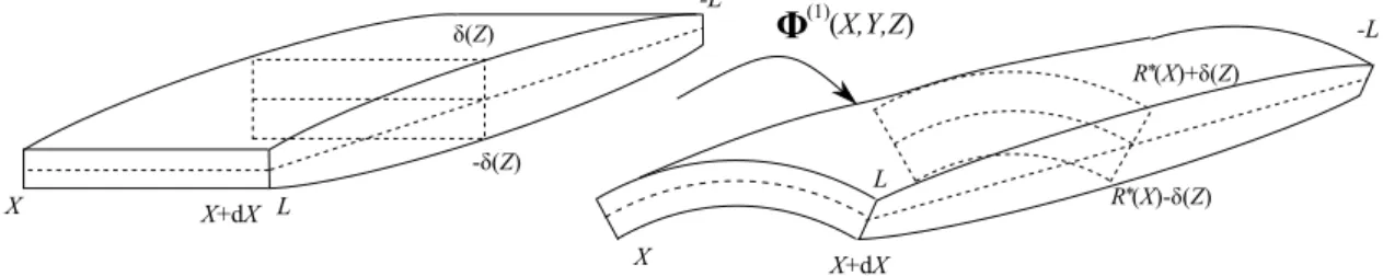
Step 1 The infinitesimal strip portion is curved arbitrarily with a trial radius of curvature R∗(X) (Z-independent). Thus, this step corresponds to a global curvature of the strip portion regardless to the axial position Z, which will be corrected in step 2. The contact between the infinitesimal strip portion and the rest of the coil is not modeled during step 1. The trial radius R∗(X) will be determined by applying weak boundary conditions in the end. This step involves large rotations and multiplicative elastic-plastic formalism is used. The mid-plane of the infinitesimal strip portion (initially flat) is transformed into a perfect cylinder of radius R∗(X). More precisely the following transformation is imposed to the strip portion:
Φ(1)
(X, Y, Z) = (R∗(X)+ Y)er+ ZeZ (3)
where the superscript (1) refers to step 1. After the transformation Φ(1), the
upper-plane has the radius R∗(X) + δ(Z) and the lower plane has the radius R∗(X) − δ(Z). This is obtained mostly by applying bending moments at both sections X and X + dX. These bending moments are due to traction profiles through the strip thickness (i.e., eY
direction). In the following, the associated Cauchy stress tensor σ(1) is evaluated as a function of the trial radius R∗(X). In figure 5 this sub-step is summarized.
Since the transformationΦ(1)is imposed, unwanted body forces fb are introduced and
calculated with divσ(1) = − f
b. However, the radial stressσ(1)rr does not vanish at the
upper and lower surfaces of the strip portion, and the resultant force of unwanted body forces compensates the unwanted resultant force of residual surface traction. There-fore, a global equilibrium is ensured through the strip portion thickness. This global equilibrium enables to use a simple transformation for modeling the curvature of the strip portion and is sufficient for the purpose of developing this simplified model. It should be mentioned that the radial Cauchy stress σ(1)rr is not meaningful because of
this global equilibrium instead of a local equilibrium, but the resultant through the strip thickness is meaningful. A schematic view of step 1 is presented in figure 5.
Figure 5: Step 1: curvature
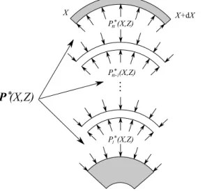
Step 2 The infinitesimal (curved) strip portion is put in contact with the rest of the coil. Con-tact pressures depend on the axial coordinate Z because of the geometrical strip profile. These contact pressures denoted by P∗(X, Z) are unknown and should be determined. An elastic-plastic model detailed in the following enables to compute the Cauchy stress tensorσ(2)(and all other quantities). Superscripts (1) and (2) are respectively related to
step 1 and step 2. Furthermore, step 2 is an additive correction under infinitesimal strain assumption to the multiplicative computation at finite strains of step 1. Thus, the final state after both steps is written without superscript and for instance the final Cauchy stress isσ = σ(1)+ σ(2). Unlike the purely elastic model developed by Weisz-Patrault
et al. (2015a) there is no analytical expression of the contact pressure as a function of the trial radius of curvature R∗(X). However, contact pressures can be determined nu-merically for each value of R∗(X). Moreover, in this contribution roughness is modeled as the possibility for each interface to interpenetrate each other via a contact law re-lating the contact pressure on the one hand and the interpenetration on the other hand. Thus, the rest of the coil cannot be modeled as a solid continuous medium (for ax-ial positions where contact is ensured) like the previous paper of Weisz-Patrault et al. (2015a). In this paper each contact should be up-dated at each time step where a new infinitesimal strip portion is added to the coil. Thus, the contact pressure P∗(X, Z) is not a scalar but a vector representing all contact pressures in the interfaces between all wound wraps (and also between the mandrel and the first wrap). A schematic view of step 2 is presented in figure 6.
Figure 6: Step 2: making contact
LetJriK(X, Z) denote the vector containing interpenetration of all interfaces, defined as
the radial position of the lower surface of the n-th wrap minus the radial position of the upper surface of the n− 1-th wrap. Thus, when a component of JriK(X, Z) is negative
there is interpenetration at the corresponding interface, and there is no contact when it is sufficiently positive). The contact law is defined in each interface as follows:
PC = f
( JrCK
)
(4) where PC denotes the contact pressure at the considered interface and JrCK the
inter-penetration of surfaces. The function f is a characterization of the roughness and deter-mined using classical literature (a proper survey is addressed in section 5). Therefore, considering a trial value of R∗(X), contact pressures are obtained by setting a trial value eP∗(X, Z) and computing the corresponding interpenetration JriK(X, Z) using the
elastic-plastic model detailed in section 4. Then, the contact law (4) is used for each interface and gives an other evaluation of contact pressures denoted by eeP
∗
(X, Z). Thus contact pressures corresponding to the trial value R∗(X) are given by the optimization problem:
∀R∗(X), P∗(X, Z) = argmin eP∗ (X,Z)≥0 eP∗(X, Z) − eeP ∗ (X, Z) (5)
In order to be compared with other models that do not take into account roughness, perfect contacts without surfaces interpenetration are also implemented as an option. In that case, considering a trial value of R∗(X), a trial value eP∗(X, Z) is set and the corresponding interpenetration JriK(X, Z) is computed using the elastic-plastic model
detailed in section 4. Then the following optimization ensuring that surfaces interpen-etration vanishes is solved:
∀R∗(X), P∗(X, Z) = argmin eP∗
(X,Z)≥0
JriK(X, Z) (6)
It should be noted that previous optimizations are done for each tested R∗(X). More-over, since all previous contacts are considered for each axial position, the number of parameters involved in latter optimizations is higher and higher. Thus, a significant issue is to reach very short computation times for the elastic-plastic problem of step 2. Semi-analytical solution has been developed to that end.
2.4. Weak boundary conditions
As mentioned in the introduction, a final optimization is needed in order to satisfy bound-ary conditions. A torque is applied to the mandrel, therefore a tangential force applied to the infinitesimal strip portion is inferred. It should be noted that the detailed tension profile through the strip thickness and width cannot be imposed and should be considered as an output. There-fore, the resultant force of tangential Cauchy stress in the infinitesimal strip portion denoted by F∗(X) should match the applied force denoted by Fa(X). Actually Fa(X) is time dependent
be-cause the applied torque decreases during the coiling process in order to avoid overstretch since the tension profile tends to concentrate because of the evolution of the contact length. However, time can be replaced by a space variable as mentioned in section 2.1. Boundary conditions are weak (because of the integration through strip thickness and width of the local stress field).
F∗(X) = ∫ L −L ∫ δ(Z) −δ(Z)σθθ (X, Y, Z)dYdZ (7)
Thus the final optimization that determines the radius of curvature R(X) solution of the winding problem is:
∀X, R(X) = argmin
R∗(X)
|F∗(X)− F
a(X)| (8)
Then, the contact pressure vector solution P(X, Z) is determined using (5), and all fields such as displacement, stress, elastic and plastic strains and hardening are determined through the elastic-plastic models of step 1 and step 2.
3. Elastic-plastic model of step 1
The elastic-plastic problem where the transformation (3) is imposed has been solved in de-tails by Weisz-Patrault and Ehrlacher (2015). Multiplicative elastic-plastic behavior has been considered with isotropic hardening. All quantities such as the Cauchy stress tensor, plastic strain etc... are computed straightforwardly. The solution relies on finding the only real root of a polynomial of degree three that can be calculated very effectively by using classical analytical solutions. However considering the complexity of this analytical form, the elastic-plastic model
of step 2 relies on interpolations of numerical results given by the present model of step 1 in-stead of a fully (and very extensive) analytical form. It has been emphasized by Weisz-Patrault and Ehrlacher (2015) that fields resulting from the present solution of step 1 are continuous but not differentiable (not smooth) at elastic/plastic interfaces. Therefore numerical results are interpolated by piece-wise polynomials of low degree (1 or 2) so that non differentiable points are not smoothed by the interpolation.
4. Elastic-plastic model of step 2
The elastic-plastic model of step 2 is an additive correction under infinitesimal strain as-sumption. In figure 6 it can be seen that a single model embraces all wound wraps. Since the assumption 4 ensures that tension profiles are the same at both sections X and X+ dX the model reduces to a cylindrical tube under plane strain assumption with inner and outer pres-sures considering pre-stress and the Tresca yield function. Many contributions focus on this kind of mechanical configuration because of its numerous engineering applications for ves-sels and piping for instance. Bree (1967) proposed an uni-axial elastic-plastic stress model in order to design nuclear reactor fuel elements. Then, Bree (1989) developed a bi-axial analyt-ical solution for an elastic-plastic pressurized tube using the Tresca yield function and where stresses are averaged through the thickness. Gao (1993) developed an analytical solution based on one-dimensional elastic-plastic behavior of a closed end thick-walled cylinder. Chu (1972) proposed a numerical approach to solve an elastic-plastic pressurized thick-walled cylinder. Durban (1988) proposed a model at finite strains using finite logarithmic strains and neglecting elastic compressibility. Then, Durban and Kubi (1992) developed a more general analytical solution based on the Tresca yield function, however considering the simple internal pressure loading only. One plastic mechanism and the corresponding corner solution are addressed. Bonn and Haupt (1995) proposed a solution for a thick-walled tube under internal pressure at finite strains based on the numerical approximation of elliptic partial differential equations. The autofrettage problem (i.e., generating residual stresses by plastic deformation and then shaping the thick walled cylinder by machining at the inner and outer surfaces) has been investigated by Parker (2001) (using numerical method) and Perry and Aboudi (2003) (using finite difference method). Several extensions of the initial thick-walled pressurized tube have been investigated. For instance Eraslan and Akis (2004) developed an analytical solution for a two-layers tube. Eraslan and Akis (2006) gave an analytical solution for a functionally graded elastic-plastic pressurized tube and Chatzigeorgiou et al. (2009) published an homogenization of a multilayer elastic-plastic pressurized tube with discontinuous material properties. Pronina (2013) devel-oped an analytical solution of an elastic-plastic pressurized tube considering mechanochemical corrosion.
In this paper, a semi-analytical solution, for a thick-walled cylinder with inner and outer pressure and considering initial residual stress, is needed and derived in the following. In this section for sake of clarity, polar coordinates (r, θ, z) are used and r = R∗(X)+ Y. Moreover, the upper and lower surfaces of the wound wrap are respectively represented in the polar co-ordinates by r = R+ and r = R−. The imposed pressures at the upper and lower surfaces are respectively denoted by P+and P−. Several mechanisms should be studied.
4.1. Elastic mechanism
The first possible mechanism is purely elastic (one can understand this calculation as an elastic test in order to check if the yield stress is exceeded). The elastic problem is computed
analytically using for instance the complex formulas established by Muskhelishvili (1953): 2µ0u(2)r = R2+R2− R2+− R2− (( P− R2+ − P+ R2− ) 3µ0 3k0+ µ0 r− P+− P− r ) σ(2) rr = R2+R2− R2 +− R2− ( P− R2 + − P+ R2 − + P+− P− r2 ) σ(2) θθ = R2 +R2− R2 +− R2− ( P− R2 + − P+ R2 − − P+− P− r2 ) σ(2) zz = 3k0− 2µ0 2(3k0+ µ0) ( σ(2) rr + σ (2) θθ ) (9) Sinceσ( j)rθ = σ( j)rz = σ ( j)
θz = 0 principal stresses are σ( j)rr,σ
( j)
θθ andσ( j)zz (where j∈ {1, 2}). Thus
the Tresca yield function is written as follows: Yf = max α∈{rr,θθ,zz} ( σ(2) α + σ(1)α ) − min α∈{rr,θθ,zz} ( σ(2) α + σ(1)α ) − k (pcum+ ∆pcum) (10)
where pcumis the cumulative plastic strain calculated during step 1 according to Weisz-Patrault
and Ehrlacher (2015) and ∆pcum is the increment of the cumulative plastic strain calculated
during step 2, thus at the beginning of step 2, ∆pcum = 0. Furthermore it is assumed that the
yield surface can be written as follows:
k(pcum+ ∆pcum)= k (pcum)+ σ0γ∆pcum (11)
The yield criterion computed using the elastic test (9) can be negative and therefore the solution is purely elastic and given by (9), but it can also be positive and therefore plastic transformations occur. Several plastic mechanisms can be distinguished depending on which components of the principal stresses are the max and the min involved in (10). There are six possible plastic mechanisms corresponding to the six edges of the Tresca hexagon:
max α∈{rr,θθ,zz} ( σ(2) α + σ(1)α ) − min α∈{rr,θθ,zz} ( σ(2) α + σ(1)α ) = σ(2) θθ + σ(1)θθ − (σ(2)rr + σ(1)rr) (mechanism 1) σ(2) rr + σ(1)rr − (σ(2)θθ + σ(1)θθ) (mechanism 2) σ(2) θθ + σ(1)θθ − (σ(2)zz + σ (1) zz ) (mechanism 3) σ(2) zz + σ (1) zz − (σ (2) θθ + σ(1)θθ) (mechanism 4) σ(2) rr + σ(1)rr − (σ(2)zz + σ(1)zz ) (mechanism 5) σ(2) zz + σ(1)zz − (σ(2)rr + σ(1)rr) (mechanism 6) (12)
The main activated plastic mechanisms are the first and the second. Thus in a plastic zone defined by r = r−pand r = r+p, an analytical solution is derived for this mechanism. Boundaries of each plastic zone are unknown and should be determined in order to verify displacement and traction continuity through elastic/plastic interfaces. The evaluation of the yield function (10) on the basis of the elastic test (9) indicates the presence of a plastic zone where a partic-ular mechanism is activated, but not the precise boundaries (usually obtained with incremental computations).
4.2. Plastic mechanisms 1 and 2
In this paper plastic mechanisms 3 to 6 are not detailed although there are no particular difficulties to address an analytical solution. It is verified during the computation on the basis of the elastic formulas (9) that these plastic mechanisms are not activated. The following piece-wise polynomials interpolation is used:
χk(r) −(σ(1) θθ − σ(1)rr ) = N ∑ j=0 Ajrj (13)
where Aj is piece-wise constant according to r and χ = 1 if the mechanism 1 is activated
and χ = −1 if the mechanism 2 is activated. The detailed analytical solution is addressed in Appendix A. Here only the final result is stated:
εp θθ = B r2 + ξ N ∑ j=0 Ajrj σ(2) rr = A + (1 + ξc) A0ln(r)+ (1 + ξc) N ∑ j=1 Ajrj j − c B 2r2 σ(2) θθ = A + (1 + ξc)A0+ A0(1+ ξc) ln(r) + (1 + ξc) N ∑ j=1 Aj(1+ j)rj j + c B 2r2 σ(2) zz = 3k0− 2µ0 2(3k0+ µ0) 2A + (1 + ξc)A0+ 2A0(1+ ξc) ln(r) + (1 + ξc) N ∑ j=1 Aj(2+ j)rj j u(2)r = C r + r 2(k0+ µ30 ) A + A0(1+ ξc) ln(r) + (1 + ξc) N ∑ j=1 Ajrj j (14) where c = χσ0γζ √ 4
3, ζ = ±1 depending on the sign of the plastic strain rate as detailed
in Appendix A andξ is defined in (A.17).
The analytical solution given for each possible plastic zone should be used for the global elastic-plastic problem where plastic zones should be determined. The elastic test is computed with (9) then the yield function (10) is evaluated on this basis. Plastic zones with identified plastic mechanisms (limited in this paper to 1 and 2) are approximated on the basis of this purely elastic calculation. Then, both boundaries of each plastic zones (r+p and r−p) are opti-mized in order to verify boundary conditions (inner and outer pressures) and displacement and normal traction continuities through each elastic/plastic interfaces. Plastic strains should also vanish at these elastic/plastic interfaces. The integration constants A, B and C involved in (14) are also determined with these latter conditions. It should be noted that integration constants A, B and C are also piece-wise constant according to r. Since each zone has two boundaries, displacement and normal traction continuities and plastic strain vanishing give six conditions. There are three integration constants and optimizations of the two boundaries r+p and r−p, there-fore five conditions can be satisfied and the last condition is automatically verified because of the constitutive equations. It should be noted that if one boundary of the considered zone is R+ or R− normal traction continuity is simply replaced by the corresponding applied normal pressure−P+or−P−.
The Tresca yield function is not differentiable at wedges of the hexagon, that is to say when the activated plastic mechanism meets another plastic mechanism. This is classically refereed
to as corner plasticity. Therefore the associated flow rule that imposes that the plastic strain rate is normal to the yield surface, should be understood at these non-differentiable points as the fact that the plastic strain rate lies in the sub-differential of the yield surface. In this paper, corner relations that determine the plastic strain rate direction when a corner is reached, are not developed. It is verified numerically during the simulation that corners are not reached during step 2.
5. Contact law
In section 4 each wound wrap has been solved considering arbitrary normal pressure at lower and upper surfaces. Excepted at the upper surface of the infinitesimal strip portion where the pressure vanishes, all other contact pressures listed in P∗(X, Z) are still unknown and should be determined as functions of R∗(X) using the methodology summarized by (5). Therefore a contact law (4) has to be chosen. A general literature survey is given by Antaluca (2005). A his-torical paper proposed by Greenwood and Williamson (1966) presents a probabilistic approach for elastic contacts and has been extended to elastic-plastic contacts by Chang et al. (1987). Then, Polycarpou and Etsion (1999) corrected the exponential approximation introduced to obtain an analytical solution. More recently, a non-statistical model based on a multiscale ap-proach has been proposed by Jackson and Streator (2006). Several classical roughness studies propose a relationship between the average contact pressure and the contact ratio, for instance Wilson and Sheu (1988), Sutcliffe (1988) and Sheu and Wilson (1994) established explicit sim-ple formulas. In this paper the empirical equation proposed by Sheu and Wilson (1994) is used PC = √23σ0A(2.571 − A − A ln(1 − A)), where PC is the average contact pressure between both
considered surfaces, A is the contact ratio andσ0is the yield stress.
Then, the contact ratio A is calculated as a function of the algebraic distance between nom-inal surfaces (denoted byJrCK) by means of composite Abbott curves A
(Jr
CK
)
that can be in-ferred from random geometrical rough surfaces. This approach is used by Collette et al. (2000) for the contact of two rough surfaces within the framework of roughness transfer in rolling process. This paper does not focus on roughness theories but extracts from classical literature a contact law taking into account roughness parameters. The method used in this paper follows the ideas of Collette et al. (2000). The composite Abbott curve between two wound wraps characterized by the interpenetration of their nominal surfaces is obtained as follows. Two geo-metrical profiles that characterize roughness (Rainµm) of each surface are randomly generated
and centered to zero (nominal surfaces are set to zero). The discretization can be refined since it is not correlated with the general numerical simulation presented in this paper, it is clearly a pre-computation. Then the geometrical profile of the upper surface is subtracted from the geometrical profile of the lower surface, this gives the algebraic distance denoted by JhK be-tween both surfaces when nominal surfaces are at the same position. For each algebraic value JrCK it then computed the proportion of points where JhK is greater or equal than JrCK which
represents the probability of having contact, that is to say the contact ratio A(JrCK
)
. Random geometrical profiles are illustrated in figure 7 for a roughness parameter Ra = 5 µm. The
corre-sponding composite Abbott curve is presented in figure 8a. It should be noted that curves such as presented in figure 8b are pre-computed and interpolated by cubic splines during the coiling simulation. Finally the contact law (4) can be written as follows and is presented in figure 8b.
PC = f (Jr CK ) = 2 √ 3σ0A (Jr CK ) [ 2.571 − A(JrCK )− A(Jr CK ) ln(1− A(JrCK ))] (15)
Thanks to the roughness model, The coiling model is able to predict the evolution of strip roughness due to coiling using the same approach as Collette et al. (2000). This completes some previous works such as those of Collette et al. (2000) that modeled roughness transfer evolution at the skin pass mill. Moreover, this possibility of roughness transfer evolution of the model is particularly interesting since coiling-uncoiling operations are present all along the steel processes.
Figure 7: Random geometrical profiles, Ra= 5 µm
(a) Composite Abbott curve, Ra= 5 µm (b) Contact law, Ra= 5 µm
Figure 8: Roughness
6. Comparisons
6.1. Comparison with previous models and effect of yield stress
In this section, the present coiling model is compared with two purely elastic models de-veloped by Hudzia et al. (1994) and Weisz-Patrault et al. (2015a). Typical coiling parameters
are set and listed in Table 2. Roughness is not taken into account for this first comparison. A perfect contact is modeled using (6) instead of (5). The yield stress is σ0 = 200 MPa for
the present model. Contact pressures and tangential stresses at the mid-plane (i.e. Y = 0) are presented in figure 9a and 9b respectively. As mentioned in the introduction tensions are more and more concentrated at the center of the strip as shown in figure 9b. It can be seen that even though the model developed by Hudzia et al. (1994) considers the wrap radius as known a priori (strip thickness added to the previous radius), tangential stresses are in very good agreement with the purely elastic model developed by Weisz-Patrault et al. (2015a). It should be noted that negative contact stress σrr can be observed when contact is lost in the model proposed
by Hudzia et al. (1994) which is excluded by construction in the present contribution and the one developed by Weisz-Patrault et al. (2015a). Since Hudzia et al. (1994) do not consider the strip curvature in the elastic computation models are only comparable at the mid-plane (i.e. Y = 0) where curvature effects vanish. However contact pressures are not in excellent agree-ment with the previous model of Weisz-Patrault et al. (2015a). This is possibly due to the fact that Hudzia et al. (1994) deals with the contact without using an explicit contact law and geo-metrical mismatch appears since each wrap radius is a priori known in order to have contact of thicker parts of wound wraps without considering displacements due to contact pressures. The present elastic-plastic model is in relatively good agreement with previous models. However, it can be noted for instance that the contact length of the first wound wrap is enlarged with the elastic-plastic behavior in comparison with the purely elastic behavior and stress magni-tudes are modified. The effects of plasticity explain differences between the previous model of Weisz-Patrault et al. (2015a) and the present contribution as shown in figure 10 where several yield stresses from 200 MPa to 400 MPa have been compared with the purely elastic model in order to show that the elastic-plastic model converges to the elastic model when the yield stress increases. Furthermore, the lower the yield stress is and the lower the contact stress amplitude is. However, at mid-plane (i.e., Y = 0) this effect is inverted for tangential stress σθθ. This is due to the fact that plastic flow concentrates near the upper surface of each wrap which limits tangential stress in this plastic zone that is large when the yield stress is low. Thus, tangen-tial stress is higher in the remaining elastic zone (especially at Y = 0) in order to balance the applied force.
Table 2: Coiling parameters
L (mm) 750 Half-width
tc (mm) 1 Strip thickness at the center (Z = 0)
te (mm) 0.952 Strip thickness at the edges (Z = ±L)
δ(Z) (mm) 1 2 ( tc− (tc− te) (Z L )2)
Half thickness parabolic profile Rext
mand (mm) 225 External mandrel radius
Rint
mand (mm) 50 Internal mandrel radius
Fa/S0 (MPa) 30 Applied force divided by the nominal surface
(mean applied stress)
E (MPa) 210000 Young’s modulus
ν (-) 0.3 Poisson ratio
k0 (MPa) 175000 Bulk modulus
µ0 (MPa) 80769.23 Shear modulus
γ (-) 1 Hardening parameter
(a) Contact pressure,−σrr (b) Tension at mid plane (i.e., Y= 0), σθθ
(a) Contact pressure,−σrr (b) Tension at mid plane (i.e., Y= 0), σθθ
Figure 10: Different yield stresses
6.2. Comparison with Finite Element Model
A Finite Element model considering elastic-plastic behavior and hard contacts (i.e., without surface interpenetration) and performed with Abaqus (2006) was available from the previous paper of Weisz-Patrault et al. (2015a). A comparison with the model developed in this paper is presented in this section. The strip is modeled with cubic elements (20 along the axial direction Z, 750 along the coiling direction X and 3 along the strip thickness Y). The yield stress is set toσ0= 200 MPa and without hardening (i.e., γ = 0) although Weisz-Patrault et al.
(2015a) presented results for σ0 = 500 MPa. Parameters are listed in table 3. Considering
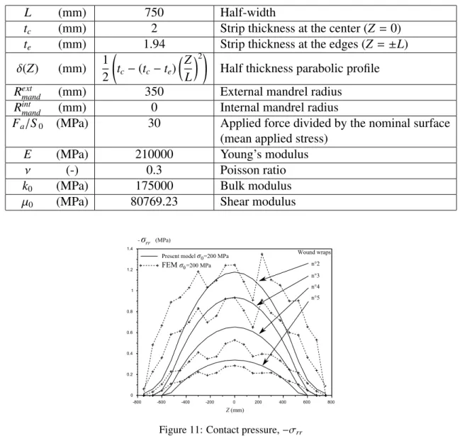
very long computation times only 5 cycles have been modeled. Contact pressures that mostly determine stresses in each wound wrap are compared in figure 11. Contacts between layers are extracted from the FEM computation which excludes the contact between the first wrap and the mandrel (that is why the first wrap is missing in figure 11). Reasonable agreement is observed between the FEM computation and the developed model, however discrepancies are not negligible. It should be noted that rather large oscillations and a clear lack of symmetry (although the problem is symmetric with respect to Z = 0) lead to put in doubt the validity of this FEM computation. This can be due to the fact that only 3 elements are used through the thickness which may not be enough to evaluate properly displacements considering that plastic zones can be much thinner that elements thicknesses. In addition an explicit scheme has been chosen so that computation times are not excessively long and a lack of stability can also explain relatively bad results obtained with the FEM. Therefore contact pressures extracted from this FEM computation give only an order of magnitude.
Table 3: Coiling parameters, comparison with FEM
L (mm) 750 Half-width
tc (mm) 2 Strip thickness at the center (Z = 0)
te (mm) 1.94 Strip thickness at the edges (Z = ±L)
δ(Z) (mm) 1 2 ( tc− (tc− te) (Z L )2)
Half thickness parabolic profile Rext
mand (mm) 350 External mandrel radius
Rint
mand (mm) 0 Internal mandrel radius
Fa/S0 (MPa) 30 Applied force divided by the nominal surface
(mean applied stress)
E (MPa) 210000 Young’s modulus
ν (-) 0.3 Poisson ratio
k0 (MPa) 175000 Bulk modulus
µ0 (MPa) 80769.23 Shear modulus
Figure 11: Contact pressure,−σrr
7. Roughness
In this section roughness is taken into account considering the simple methodology pro-posed in section 5. Parameters are listed in Table 2 with a yield stress set to σ0 = 600 MPa
(no significant plastic deformations) in order to see the effect of roughness only. Two com-putations have been done, the first one with perfect contacts and the second one considering roughness with Ra = 5 µm. This value is not realistic and has been chosen in order to
empha-size roughness effects after only 70 wraps. Contact pressures and tension at mid-plane (i.e., Y = 0) after 10 wraps are presented in figures 12a and 12b and after 70 wraps in figures 13a and 13b. As mentioned in the introduction Wilkening (1965) gave experimental evidence that the model proposed by Sims and Place (1953) (purely elastic not taking into account rough-ness) overestimates stresses after 55 wound wraps. The model developed in this paper presents no significant discrepancies between perfect and rough contacts after 10 wraps. One can ob-serve that the overestimation of contact pressure and tension when roughness is not taken into account becomes more substantial after 70 wraps. This confirms the significance of roughness.
One can also mention that tension of the first wrap in figure 13b locally decreases at the center. This is due to accumulation of pressure at the center. Indeed contacts are more and more localized at the center, thus pressures increases where contacts localize, especially for the first wound wraps that are compressed by all the other wraps.
(a) Contact pressure,−σrr (b) Tension at mid plane (i.e., Y= 0), σθθ
Figure 12: Effect of roughness after 10 wraps
(a) Contact pressure,−σrr (b) Tension at mid plane (i.e., Y= 0), σθθ
Figure 13: Effect of roughness after 70 wraps
8. Residual stress : uncoiling model
As mentioned in the introduction, this paper aims at developing a numerical tool for eval-uating residual stress field after coiling, in order to develop strategies to minimize flatness defects. Elastic-plastic computations have been developed in order to model the evolution of irreversible strain that causes residual stress after uncoiling. This section presents a very sim-plified residual stress computation that takes into account uncoiling, assuming that the latter
process is purely elastic. It consists in making the strip mid-plane perfectly flat again. Obvi-ously the strip is not perfectly flat after uncoiling because residual stresses are in fact relaxed by out of plane deformations. However the interesting quantity is the residual stress profile when the strip mid-plane is perfectly flat in order to evaluate the flatness defect that will be created by this relaxation of residual stress including buckling analysis. This simple uncoiling calculation consist in releasing contact pressure by applying the opposite contact stress in all interfaces using the elastic formulas (9). At this stage the strip mid-plane is not a perfect cylinder because of the irreversible plastic deformations during step 2. A perfect cylinder is obtained by shifting the stress profiles through the strip thickness so that the elastic zone does not present residual stresses. The stress fieldσu = σurrer⊗er+σθθu eθ⊗eθ+σuzzez⊗ez(where u means uncoiling) at the
end of this step is the sum of the stress field at the end of coiling process and the stress field due to releasing contact pressures (computed with (9)) and considering the latter stress shift. It can be seen as an initial stress before applying the inverse transformation gradient corresponding to the curvature of step 1 defined by Weisz-Patrault and Ehrlacher (2015). This ensures that the mid-plane of the strip is flat. Thus, an elastic tensor is responsible for this stress fieldσu and
denoted by Eu0 which is a diagonal tensor considering that the stress tensor is diagonal. One can obtain Eu0.tEu
0from the known stress fieldσ
u:
Eu0.tEu0= Aurrer⊗ er+ Auθθeθ⊗ eθ+ Auzzez⊗ ez (16)
where (Au
rr, Auθθ, Auzz) are known functions determined as detailed in Appendix B. From the
latter equation, the purely elastic uncoiling gives the residual stress field: σres XX = µ0 3(JuJeu )5 3 ( 2 eJu2Aθθ− Arr− Azz ) + k0 ( JuJeu− 1 ) σres YY = µ0 3(JuJeu )5 3 ( −eJu2Aθθ+ 2Arr− Azz ) + k0 ( JuJeu− 1 ) σres ZZ = µ0 3(JuJeu )5 3 ( −eJu2Aθθ− Arr+ 2Azz ) + k0 ( JuJeu− 1 ) (17)
where the superscript res means residual. For instance, considering coiling parameters listed in table 2 where the applied force is set to Fa/S0 = 30 MPa, the yield stress is σ0 = 200 MPa
and the hardening parameter isγ = 1, it is obtained (ater 5 cycles) the residual stress profiles presented in figures 14a and 14b. Different zones are clearly identified with gradient discon-tinuities. These zones are indicated in figures 14a and 14b for the first wound wrap. During step 1 that consists in a simple curvature, the lower surface is under compression and the upper surface under tension that lead to plastic deformations. During step 2 contact pressure is applied and the whole thickness is under tension. Without step 1, this tension would not be sufficient to initiate plastic deformations however since the upper surface is already under tension even very limited contact pressure is sufficient to lead to plastic deformations in a slightly thicker plastic zone. It should be noted that slope changes near the lower surface and upper surface are almost aligned for the 5 wound wraps. This is due to the fact that these slope changes correspond to plastic deformations during step 1 that are almost the same for these wound wraps (there is no significant variation of the radius of curvature R(X)). However the slope change corresponding to plastic deformations during step 2 occurs more and more near the strip center (i.e., Y = 0) because contact pressure at Z= 0 localize as shown in figure 15. It should be noted that the lat-ter figure presents the contact pressure at the lower surface of the wound wrap n aflat-ter n cycles
(contact pressure of the last wound wrap). This is different from previous figures such as 9a, 10a, 11, 12a, 13a where contact pressures for the wound wrap n are given after that all cycles are computed giving contact pressures in the whole final coil.
An interesting quantity (18) is the average residual profile calculated through the strip thick-ness and plotted along the coil width. This enables to understand major flatthick-ness defect as pre-sented in figure 2. Σres XX(Z)= 1 2δ(Z) ∫ δ(Z) −δ(Z)σ res XX(Y, Z)dY (18)
(a) Residual stress profiles σresXX through thickness at Z= 0
(b) Residual stress profiles σresZZ through thickness at Z= 0
Figure 14: Residual stress through the thickness
Figure 15: Contact pressure,−σrrfor the last wrap
9. First results
In this section several numerical simulations have been performed. The influence of three coiling parameters have been tested namely: applied forces, strip geometrical profiles and man-drel’s radii. Parameters are listed in table 2 and the tested parameters are listed in table 4. For
each test five cycles are modeled and results for the fifth wrap are presented in figures 16, 17 and 18.
Test 1 Contact pressures, tangential stress and contact length increase when the applied force increases. Stresses keep the same distribution along the coil width (with a scale factor), so stresses do not localize, the increase being only due to the applied force. Thus the higher the stress peak is and the higher the contact length is. Plastic zones generated during step 2 are wider and wider when plastic deformations during step 1 do not evolve since the mandrel’s radius is the same for all tested applied forces (thus the radius of curvature does not evolve much).
Test 2 The strip crown is increased by decreasing the thickness te at the edges of the strip.
When there is no strip crown (i.e., te = tc = 1 mm) the contact is ensured all along the
coil width. The strip crown is responsible for the barrel shape (i.e., the contact length decrease) as explained in the introduction, thus the more severe the crown is and the shorter the contact length is. Therefore contact pressure and tangential stress localize where the contact is ensured which explains that stress peaks are higher and higher. Plastic deformations during step 1 is similar to the test 1 since the radius of curvature does not evolve much. At the center of the coil where contact is ensured for all tests, plastic deformations during step 2 are also similar to the test 1. However one can see in figures 16e and 17e that the evolution of the average residual stress through thickness defined by (18) have different profiles along the coil width if stresses localize at the center (test 2) or not (test 1).
Test 3 The contact pressure and tangential stress peaks increases when the mandrel’s radius decreases. This is due to the fact that the contact length decreases so that pressures lo-calize alike the test 2. Therefore plastic deformations where stresses concentrate present significant variations during step 2 but also in step 1 because the radius of curvature evolves significantly. For a mandrel’s radius of 500 mm the curvature is not sufficient to generate plastic deformations. When the curvature increases for mandrel’s radii of 300 mm and 100 mm plastic deformations during step 1 are more and more severe: plas-tic zones are larger and gradients are higher. But since contact pressure and tangential stress localize more and more at the center of the coil (Z = 0) plastic elongations during step 2 are also more and more severe with higher gradients. This gradient increase is due to the fact that at the end of step 1 larger plastic zones (i.e., a smaller elastic zone) are obtained for smaller mandrel’s radii, thus the additional stress peak during step 2 is not only higher but also applied on a smaller elastic region. For tests 1 and 2 gradients of plastic deformations during step 2 are constant because the stress peak is applied on the same elastic region, plastic zones being larger and larger because of the stress peak increase.
(a) Contact pressure for the 5th wound wrap (b) Tangential stress for the 5th wound wrap
(c) Contact length (d) Residual stress along thickness
(e) Average residual stress along width
(a) Contact pressure for the 5th wound wrap (b) Tangential stress for the 5th wound wrap
(c) Contact length (d) Residual stress along thickness
(e) Average residual stress along width
(a) Contact pressure for the 5th wound wrap (b) Tangential stress for the 5th wound wrap
(c) Contact length (d) Residual stress along thickness
(e) Average residual stress along width
Table 4: Varying parameters for each test
(a) Test 1: Applied forces Fa/S0(MPa)
10 20 30 40
(b) Test 2: Strip profiles te(mm) 1 0.9 0.8 0.7 0.6
(c) Test 3: Mandrel’s radii Rext mand(mm) 100 300 500 10. Conclusion
This paper presents a coiling model taking into account elastic-plastic behavior at finite strain considering isotropic hardening. Multiplicative formalism is used as well as an additive correction under infinitesimal strain assumption. The modeling strategy involves a fully ana-lytical solution (step 1) and a semi-anaana-lytical solution (step 2). The global simulation relies on several optimization problems in order to determine contact pressures and the radius of curva-ture that enables to match the tangential applied force. Roughness has been considered using composite Abbott curves and empirical laws. This part being an external input of the model, one can consider other options. Comparisons with already existing models have been addressed and good agreement is observed for large yield stress. However, for lower yield stress the nu-merical solution presents more discrepancies with purely elastic models found in the literature showing the interest of an elastic-plastic computation. A simple purely elastic uncoiling model has been proposed in order to quantify residual stresses after unwinding and releasing tension. Results show that the coiling process can be responsible for significant residual stress fields due to plastic deformations. Since the model is based on analytical or semi-analytical sub-steps, reasonable computation times are obtained. For instance 5 cycles are computed within 1 minute with the freeware Scilab (2012), where a classical FEM computation using explicit in-tegration scheme (with stability issues) takes several weeks. However computation times grow exponentially (due to larger optimization problems) and 70 cycles are computed within around 24 hours. The code should be optimized and re-written in a compiled language such as C++ in order to obtain shorter computation times.
Acknowledgment
Authors gratefully acknowledge Eliette Mathey (ArcelorMittal Global Research & Devel-opment, Maizi`eres Process, 57283 Maizi`eres-l`es-Metz, France) for providing results of her Finite Element simulation of coiling process used in section 6.2.
Appendix A. Analytical solution of step 2
Thus, let consider a plastic zone where the plastic mechanism 1 or 2 is activated, thus: max α∈{rr,θθ,zz} ( σ(2) α + σ(1)α ) − min α∈{rr,θθ,zz} ( σ(2) α + σ(1)α ) = χ[σ(2) θθ + σ(1)θθ − (σ(2)rr + σ (1) rr) ] (A.1)
whereχ = 1 if the mechanism 1 is activated and χ = −1 if the mechanism 2 is activated. In these conditions, the Tresca yield function (10) vanishes and reduces to:
σ(2) θθ − σ(2)rr = K(r) + χσ0γ∆pcum (A.2) where: K(r)= χk(pcum)− ( σ(1) θθ − σ(1)rr ) (A.3) It should be noted that K(r) is known from step 1. Letεpdenote the plastic strain of step 2. At the beginning of this step, εp = 0. The total plastic strain of both steps (1 and 2) is obtained
by adding the plastic strain of step 1 and the plastic strain of step 2. The flow rule is associated therefore the plastic strain rates are normal to the Tresca yield surface corresponding to this plastic mechanism, thus:
˙ εp
θθ= −˙εrrp and ε˙zzp = 0 (A.4)
Hence the cumulative plastic strain rate for this step: ˙pcum = √ 2 3 ([ ˙ εp rr ]2 +[ε˙θθp]2+[ε˙zzp ]2) = ζ √ 4 3ε˙ p θθ (A.5)
whereζ is the sign of ˙εθθp. An initial guess is of courseζ = χ which means that tangential plastic flow is positive when the strip is under tension. If displacement and normal stress continuity is not verified in the end the other value is set forζ. After integration (considering that at the beginning of step 2,εθθp = 0): ∆pcum= ζ √ 4 3ε p θθ (A.6)
The equilibrium can be written as follows: dσ(2)rr dr + σ(2) rr r − σ(2) θθ r = 0 (A.7)
Using the yield criterion (A.2), the latter equilibrium (A.7) reduces to: dσ(2)rr dr = K(r) r + χσ0γζ √ 4 3 εp θθ r (A.8)
Hence after integration: σ(2) rr = A + ∫ r K(ρ) ρ dρ + χσ0γζ √ 4 3 ∫ r εp θθ(ρ) ρ dρ σ(2) θθ = A + ∫ r K(ρ) ρ dρ + χσ0γζ √ 4 3 ∫ r εp θθ(ρ) ρ dρ + K(r) + χσ0γζ √ 4 3ε p θθ (A.9)
The Cauchy stress tensor can be written as follows: σ(2) rr = ( k0+ 4µ0 3 ) du(2)r dr + ( k0− 2µ0 3 ) u(2)r r − 2µ0ε p rr σ(2) θθ = ( k0− 2µ0 3 ) du(2)r dr + ( k0+ 4µ0 3 ) u(2)r r − 2µ0ε p θθ σ(2) zz = ( k0− 2µ0 3 ) ( du(2)r dr + u(2)r r ) + 2µ0 ( εp rr+ ε p θθ ) (A.10)