Publisher’s version / Version de l'éditeur:
Vous avez des questions? Nous pouvons vous aider. Pour communiquer directement avec un auteur, consultez la Questions? Contact the NRC Publications Archive team at
[email protected]. If you wish to email the authors directly, please see the first page of the publication for their contact information.
https://publications-cnrc.canada.ca/fra/droits
L’accès à ce site Web et l’utilisation de son contenu sont assujettis aux conditions présentées dans le site LISEZ CES CONDITIONS ATTENTIVEMENT AVANT D’UTILISER CE SITE WEB.
Student Report (National Research Council of Canada. Institute for Ocean Technology); no. SR-2006-20, 2006
READ THESE TERMS AND CONDITIONS CAREFULLY BEFORE USING THIS WEBSITE.
https://nrc-publications.canada.ca/eng/copyright
NRC Publications Archive Record / Notice des Archives des publications du CNRC :
https://nrc-publications.canada.ca/eng/view/object/?id=7353d0c9-320c-4c00-afcf-bf0e1b802230 https://publications-cnrc.canada.ca/fra/voir/objet/?id=7353d0c9-320c-4c00-afcf-bf0e1b802230
NRC Publications Archive
Archives des publications du CNRC
For the publisher’s version, please access the DOI link below./ Pour consulter la version de l’éditeur, utilisez le lien DOI ci-dessous.
https://doi.org/10.4224/8895117
Access and use of this website and the material on it are subject to the Terms and Conditions set forth at
Effect of free surface on CFD predictions for a Wigley hull form at increasing yaw angles
DOCUMENTATION PAGE REPORT NUMBER
SR-2006-20
NRC REPORT NUMBER DATE
August 2006 REPORT SECURITY CLASSIFICATION
Unclassified
DISTRIBUTION
Unlimited TITLE
EFFECT OF FREE SURFACE ON CFD PREDICTIONS FOR WIGLEY HULL FORM AT INCREASING YAW ANGLES
AUTHOR(S)
Amanda Collier, David Molyneux
CORPORATE AUTHOR(S)/PERFORMING AGENCY(S)
Institute for Ocean Technology, National Research Council, St. John’s, NL PUBLICATION
SPONSORING AGENCY(S)
Institute for Ocean Technology, National Research Council, St. John’s, NL
IMD PROJECT NUMBER NRC FILE NUMBER
KEY WORDS
CFD, Fluent, Free Surface, Yaw Angle
PAGES iii, 29 FIGS. 25 TABLES 7 SUMMARY
The effect of the free surface is of great interest for marine technology, however including the free surface in computational fluid dynamic (CFD) predictions complicates the problem. This study examines the processes needed to include the free surface in CFD predictions for a simplified ship hull at yaw angles up to 40 degrees. The CFD predictions were compared to experiment data whenever possible and to predictions for the same flow conditions in a fluid with no free surface. The results are compared using calculated force coefficients, flow patterns and where applicable, free surface wave profiles.
ADDRESS National Research Council
Institute for Ocean Technology Arctic Avenue, P. O. Box 12093 St. John's, NL A1B 3T5
National Research Council Conseil national de recherches Canada Canada
Institute for Ocean Institut des technologies Technology océaniques
EFFECT OF FREE SURFACE ON CFD PREDICTIONS FOR
WIGLEY HULL FORM AT INCREASING YAW ANGLES
SR-2006-20
Amanda Collier, David Molyneux
TABLE OF CONTENTS
INTRODUCTION .……… 1
MESHING STRATEGY ...……… 1
CFD SOLUTIONS OBTAINED USING FLUENT ………... 5
SUMMARY OF CALCULATED FORCES AND MOMENTS ………... 5
EVALUATION OF RESULTS AGAINST PUBLISHED EXPERIMENTAL AND NUMERICAL RESULTS ………. 8
Wave Contours ……….. 8
Zero Yaw ………. 8
Yaw Angle 10 Degrees ……… 9
Wave Profiles ………. 11
Zero Yaw ………. 11
Yaw Angle 10 Degrees ……… 11
Force Coefficients ……….. 12
FREE SURFACE EFFECTS ……… 14
Velocity Magnitude Contours ……….. 14
Force Coefficients ………. 16
Velocity Fields ……… 19
EFFECT OF FROUDE NUMBER ON DISCREPANCY BETWEEN FREE SURFACE CASE AND NO FREE SURFACE CASE AT 40o YAW … 26 CONCLUSIONS ……… 28
EFFECT OF FREE SURFACE ON CFD PREDICTIONS FOR WIGLEY HULL FORM
AT INCREASING YAW ANGLES
INTRODUCTION
Computational fluid dynamics (CFD) has become an integral part of designing ship hulls and analyzing hydrodynamics. The computations allow the hull designer to predict the wave patterns around a ship hull and the forces and pressures caused by the flow. Most recently it has become possible to include the effect of the free surface on these parameters within commercial CFD codes. Traditionally, the free surface effects were often ignored due to the complexity of the problem. Increased computer capacity and improved numerical schemes have made the calculation of free surface viscous flows a realistic goal for CFD studies.
In marine cases, the free surface is especially important because ships operate at the interface between two fluids. However, including the free surface is challenging, making the design of the mesh and the definition of the problem more complex and increasing the number of iterations for the CFD program to reach a solution. The work described in this report is an attempt to determine how significant the free surface is to the computed forces and flow patterns for a ship hull with a yaw angle, given that in most practical situations a ship cannot sustain a high yaw angle at Froude numbers over 0.2, and below this speed, the waves generated are generally small.
The chosen hull shape for this study was Wigley hull, defined by second order curves of x, y and z. It is a very simple shape, simplifying the mesh and the time required to design it. Despite its geometric simplicity, this hull has been well studied by other researchers, with data from model experiments and CFD predictions available.
For this study, the effect of free surface flow on wave patterns, velocity vectors and forces at the hull will be examined at several different yaw angles. The study described in this report was carried out using the commercial RANS based CFD program Fluent (Fluent Inc., 2005) and meshes for this program were created using Gambit (Fluent Inc., 2005), the meshing program supplied by the same company. To study the free surface effects, a mesh with fine definition around the free surface was designed, and CFD predictions for several different yaw angles were obtained. These results were compared to the results of a single-phase system at the same flow speeds, using the same mesh but with the cells above the free surface removed. Both sets of results were compared to experimental results and/or published computational results wherever possible.
MESHING STRATEGY
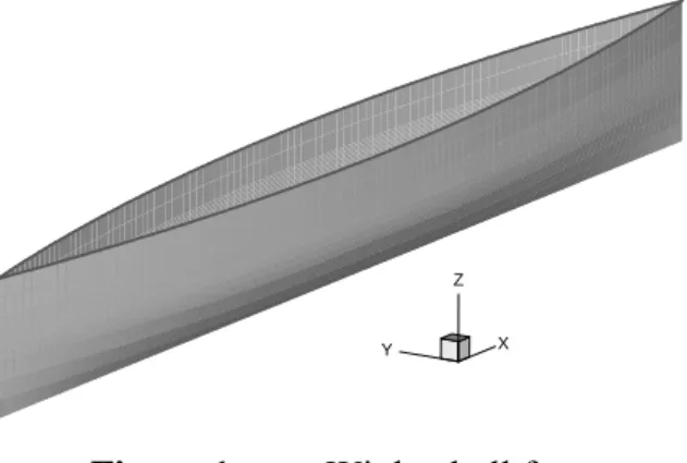
Before meshing could begin, a file defining the Wigley hull surface [1] was imported into Gambit, with the surfaces being imported as virtual surfaces. The hull shape is shown in Figure 1. In order to obtain acceptable results (for example, good definition at the free
X Y
Z
Figure 1: Wigley hull form
surface and around the hull), several meshes were developed, with each mesh improving on the deficiencies of the previous mesh. This process was somewhat trial and error, and only the final mesh used to carry out the study will be described here.
The origin was oriented so that the x-axis was positive towards the stern, the y-axis was positive to starboard and the z-axis was positive upwards. The origin itself lies at the center of the hull. Hexahedral meshes were used for the entire domain, thus all faces had to be four-sided, and all volumes made up of six faces. As the main objective of the proposed numerical experiments was to evaluate the effect of the free surface, it was particularly important to create a very fine grid in the area where the free surface was expected to exist.
The free surface is initially assumed (by Fluent) to be at z = 0 (the waterline of the hull when stationary in calm water), thus the volumes around this plane had to be meshed with extremely small cells. Beginning at this level, a very small volume was created just above the free surface, and just below. The surface of the imported hull was split into eight faces (four on each side), thus each side of the hull had four volumes along the x-direction. These faces were further split to create the fine mesh at z=0. In the end, 32 faces were used to define the hull. Once the volumes immediately above and below the free surface were created and meshed with a very fine grid, the mesh was continuously built out from the hull, with the meshing becoming coarser as the distance from the hull increased.
One other area that was finely meshed was the region just below the bottom of the hull, below the keel. This was done in an attempt to achieve accurate predictions of the velocity vectors in the region where the flow was expected to separate from the hull when a yaw angle was introduced. The final free surface mesh had boundaries of 1 ≤ x ≤2, -1.5 ≤ y ≤-1.5, -0.5 ≤ z ≤0.05 for a hull with an overall length of 1.0. A total of 870 578
were -1 ≤ x ≤2, -1.5 ≤ y ≤1.5, -0.5 ≤ z ≤0 for a hull with an overall length of 1.0. This mesh had a total of 627 626 elements.
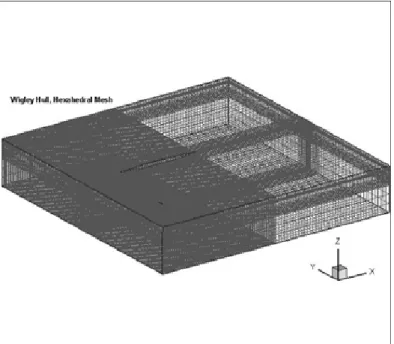
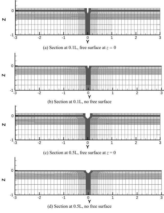
In order to compare with published data from experiments using a 2m model, the mesh was scaled within Fluent, using the scaling function to double the size of the domain. This scaled mesh is shown in Figures 2 and 3 below, along with representative sections parallel to the yz-plane [Figure 4].
Figure 2: Hexahedral Mesh for Wigley Hull, origin in center of hull,
x-axis positive towards stern, Free surface at z = 0.
(a) Section at 0.1L, free surface at z = 0
(b)Section at 0.1L, no free surface
(c) Section at 0.5L, free surface at z = 0
(d) Section at 0.5L, no free surface
Y Z -3 -2 -1 0 1 2 3 -1 0 Y Z -3 -2 -1 0 1 2 3 -1 0 Y Z -3 -2 -1 0 1 2 3 -1 0 Y Z -3 -2 -1 0 1 2 3 -1 0
Figure 4: Representative Sections of hexahedral meshes, free surface case shown in (a)
CFD SOLUTIONS OBTAINED USING FLUENT
For the free surface case, the upstream end of the domain was defined as a pressure inlet, while the downstream end was defined as a pressure outlet. The hull surface was defined as a no-slip wall, and the side, lower, and upper surfaces were defined as walls with zero shear force. For cases with non-zero yaw angle, the upstream side was changed to a pressure inlet, the downstream side to a pressure outlet. For the case with no free surface, the conditions are the same, except the inlet(s) are defined as velocity inlets rather than pressure inlets.
Fluent was used to obtain predictions of the flow and x-, y- and z-forces at the hull. Flow entered the domain through a pressure inlet on the upstream boundaries (or velocity inlet in the case of no free surface) and exited through a pressure outlet on the downstream boundaries. Yaw angles were controlled by changing the x and y components of the direction vector, where the cosine of the yaw angle gave the x-component and sine of the angle gave the y-component.
The multiphase model utilized was the ‘Volume of Fluid’ (VOF) model. This model is designed for situations where the interface between two (or more) immiscible fluids is of specific interest. There is a single set of momentum equations for both fluids and the volume fraction of each computational cell is tracked throughout the domain[2]. The volume fraction can lie between 1 and 0, where a value of 0 indicates Fluid 0 is present and a value of 1 indicates Fluid 1 is present. Intermediate values are indicative of the interface between the two fluids (i.e. the free surface) [3]. The standard k-ε turbulence model was used, applying the default settings within Fluent, summarized in Table 1. Turbulence intensity and turbulence viscosity ratio were set at 1% and 1 respectively. The flow was solved for the steady state case. The convergence limit for all parameters was set to 10-3 and all solutions converged within these limits.
Table 1: Parameters for κ−ε Turbulence Model Cµ 0.09
C1-ε 1.44
C2-ε 1.92
TKE Prandtl Number 1
SUMMARY OF CALCULATED FORCES AND MOMENTS
The forces and moments predicted by Fluent are summarized in Table 2 and 3 respectively. These values were used to calculate the non-dimensional force
coefficients, which are presented in later sections. Using Table 2, it can be observed that as speed increases, the magnitude of Fx and Fy increase, while Fz decreases. As the yaw angle increases from 0o to 40o , Fx decreases, and Fy increases. The forces in the x and y direction are similar for the cases with and without the free surface. However, as the angle increases the discrepancy becomes larger. For example, at 0o yaw, the force in the x-direction differs by 3% but at 30o yaw, the difference is almost 45%.
The value of all the moments (Mx, My and Mz) increase as the speed is increased and as the yaw angle is increased.
The number of iterations required for each solution is included in Tables 2 and 3. They demonstrate the significant time commitment needed when the free surface is included. In most cases, the number of iterations for the free surface case is 4-5 times the number required without the free surface.
Table 2: Summary of Forces
# Itterations Fx (N) Fy (N) Fz (N)
Yaw Angle (o) Speed (m/s) Fn FS nFS FS nFS FS nFS FS nFS
0 1.18266 0.267 1031 205 2.2427 2.1772 -0.0094 0.0002 207.650 -7.4025 0 1.32883 0.300 1050 200 2.6880 2.7064 -0.0174 0.0011 204.020 -9.3462 0 1.39971 0.316 983 197 3.1254 2.9842 -0.0191 0.0010 201.426 -10.3733 10 1.18266 0.267 1045 200 2.2670 2.1677 18.977 18.811 199.938 -13.630 10 1.39971 0.316 1047 291 3.4709 2.8293 27.312 26.890 193.922 -18.559 15 1.18266 0.267 1067 207 2.0334 2.0720 35.292 35.447 195.979 -19.833 20 1.18266 0.267 1314 250 2.0135 1.8823 53.874 57.515 192.310 -27.024 30 1.18266 0.267 1645 609 1.9054 0.8516 89.267 112.83 181.080 -35.329 40 1.18266 0.267 1675 935 1.7097 -1.101 119.52 155.43 173.615 -38.070
Table 3: Summary of Moments
# Itterations Mx (Roll) My (Pitch) Mz (Yaw)
Yaw Angle (o) Speed (m/s) Fn FS nFS FS nFS FS nFS FS nFS
0 1.18266 0.267 1031 205 0.00002 -0.000002 -0.2455 -0.0299 0.002 0.0011 0 1.32883 0.300 1050 200 -0.00046 0.00002 -0.9707 -0.0322 -0.006 0.0013 0 1.39971 0.316 983 197 -0.0006 -0.00002 -0.2455 -0.0332 0.002 0.0013 10 1.18266 0.267 1045 200 0.7917 1.0276 -1.339 0.216 -7.804 -5.9755 10 1.39971 0.316 1047 291 1.1237 1.4132 -1.729 0.193 -11.183 -8.627 15 1.18266 0.267 1067 207 1.4848 1.8633 -2.447 0.255 -12.261 -9.1476 20 1.18266 0.267 1314 250 2.2963 2.8756 -3.130 0.215 -17.949 -12.352 30 1.18266 0.267 1645 609 3.7904 4.7957 -5.029 -1.99 -24.775 -23.240 40 1.18266 0.267 1675 935 4.9113 6.420 -7.11 -7.89 -29.566 -38.176 FS = Free Surface nFS = No Free Surface
EVALUATION OF RESULTS AGAINST PUBLISHED EXPERIMENTAL AND NUMERICAL RESULTS
Wave Contours
ZERO YAW
The wave contours at the free surface are compared with published experimental and numerical results. Figure 5 below compares the free surface contours calculated using Fluent with experimental data (model test, YNU [4]), for Fn=0.267. Figure 6 compares
the current results with the numerical results published by Lee and Soni [5], who used a higher-order finite analytic scheme (again Fn=0.267).
(a) Experimental wave contours (YNU Model Test)
(b) Wave contours computed using Fluent
Figure 5: Comparison of Fluent wave contours at the free surface with
(a) Wave contours published by Lee and Soni x/Length y/ Le ng th -1 0 1 -1 -0.8 -0.6 -0.4 -0.2 0 Z 0.022 0.021 0.02 0.019 0.018 0.017 0.016 0.015 0.014 0.013 0.012 0.011 0.01 0.009 0.008 0.007 0.006 0.005 0.004 0.003 0.002 0.001 0 -0.001 -0.002 -0.003 -0.004 -0.005 -0.006 -0.007 -0.008 -0.009 -0.01 -0.011 -0.012
(b) Wave contours computed using Fluent
Figure 6: Comparison of free surface wave contours with published
computational data (Fn = 0.267, α = 0o)
YAW ANGLE 10 DEGREES
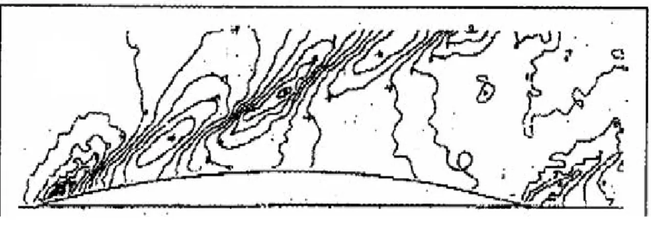
For the 10o yaw angle case, the wave contours are compared with experimental and computational data [6] in Figure 7. Again, Fn = 0.267, and positive and negative contours
are represented by solid and dotted lines respectively. In all cases the wave contours compare quite well with published data. One possible improvement may be to refine the mesh further from the hull, as the area around the hull shows excellent agreement, but the area further away (>0.5L) could benefit from better definition.
(a) Experiment
Figure 7: Wave Contours (Fr=0.267, α=10o, distance between contours lines = 0.002)
(c) Fluent Results
WAVE PROFILES
ZERO YAW
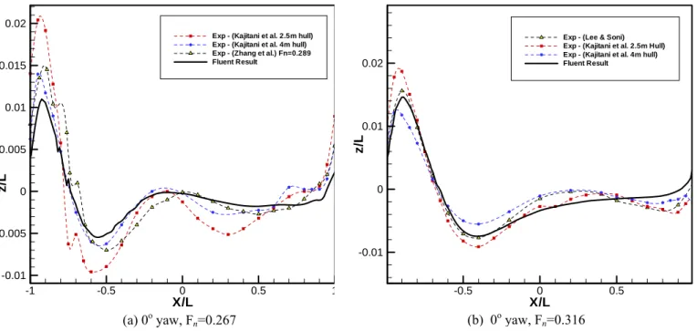
The figures below show the free-surface profiles along the hull. The profiles for 0 and 10 degree yaw angles are compared with available experimental and computational results. Figure 8(a) illustrates the profile for 0o yaw, Fn=0.267. The results obtained from Fluent
are compared with the model data given by Kajitani et al. [7] and by Zhang [2] (note that Zhang’s results are for Fn=0.289). Figure 8(b) shows another profile for 0o yaw, but for
Fn=0.316. This result is again compared to available experimental results [5],[7]. The
position of maximum and minimums agree very well in both cases. For Fn=0.267 the
amplitude of the waves at the hull appears to be underestimated. The Fluent result for the higher Froude number (Fn=0.316) shows better agreement, falling within the range of the
experimental results. X/L z/ L -1 -0.5 0 0.5 1 -0.01 -0.005 0 0.005 0.01 0.015 0.02
Exp - (Kajitani et al. 2.5m hull) Exp - (Kajitani et al. 4m hull) Exp - (Zhang et al.) Fn=0.289 Fluent Result X/L z/ L -0.5 0 0.5 -0.01 0 0.01 0.02
Exp - (Lee & Soni) Exp - (Kajitani et al. 2.5m Hull) Exp - (Kajitani et al. 4m hull) Fluent Result
Figure 8: Wave profiles along the Wigley hull
(b) 0oyaw, F
n=0.316 (a) 0o yaw, F
n=0.267
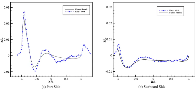
YAW ANGLE 10 DEGREES
The wave profiles for 100 yaw angle (Fn=0.267) are compared to experimental results
[Figure 9] from YNU [6]. The port and starboard sides of the Wigley hull are the pressure and suction sides, respectively. Both sides show quite good agreement with the experimental results, although again, a slight underestimation of the height of the waves occurred in the Fluent results.
Force Coefficients
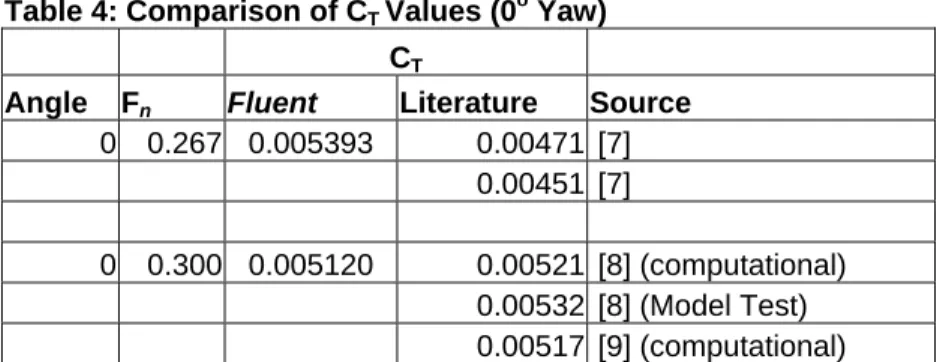
The values of coefficients can also be compared to evaluate the accuracy of results. At zero yaw angle, the most commonly used coefficient is CT, which is calculated according to the equation
CT = Drag ½ ρVs2S
where S = wetted surface area. In the cases where the yaw angle is greater than zero, two coefficients can be studied – one using the x-component of the force and the other the y-component. These are referred to as longitudinal and lateral forces, respectively.
Longitudinal Force = Fx Lateral Force = Fy
½ ρVs2S ½ ρVs2S X/L z/ L -1 -0.5 0 0.5 1 -0.01 0 0.01 0.02 0.03 Fluent Result Exp - YNU X/L z/ L -1 -0.5 0 0.5 1 -0.01 0 0.01 0.02 0.03 Exp - YNU Fluent Result
Figure 9: Wave profile along the Wigley hull 10o yaw, Fn=0.267
(b) Starboard Side (a) Port Side
In general, the forces calculated using Fluent are higher than those reported in the literature (see Tables 4 and 5), both experimental and computational values. This is possibly caused by the absence of sinkage and trim in the Fluent model, as it is fixed within the grid domain.
Table 4: Comparison of CT Values (0 o
Yaw)
CT
Angle Fn Fluent Literature Source
0 0.267 0.005393 0.00471 [7] 0.00451 [7] 0 0.300 0.005120 0.00521 [8] (computational) 0.00532 [8] (Model Test) 0.00517 [9] (computational)
Table 5: Comparison of Coefficients (10o Yaw)
Angle Fn Coefficient Fluent Literature Source
10 0.267 Lateral (linear) 0.04563 0.03319 [6] (Computational) Lateral (nonlinear) 0.03651 [6] (Computational)
Longitudinal (linear) 0.00545 0.001254 [6] (Computational) Longitudinal (nonlinear) 0.000916 [6] (Computational)
Table 4 suggests that the force coefficients are more accurate at higher Froude numbers. At Fn=0.267, the predicted value differs from the literature values by 15% and 20%. In
contrast, at Fn=0.300, the predicted value is within 4% of the model test data. At 10o
yaw, the values are quite different than the published numerical values, differing by at least 25% for the lateral coefficient. For the longitudinal coefficient, the value predicted by Fluent is over four times greater than the computational value published by Tahara and Longo [6]. Unfortunately, no model data is available to provide a true measure of accuracy.
FREE SURFACE EFFECTS
The free surface is particularly important in marine technology as ships operate at the interface between air and water. Often however, this surface has been omitted in CFD studies, as it complicates the design of the mesh, and it greatly increases the time and computer power required to obtain a solution. How much does inclusion of the free surface in the problem change the CFD predictions? Is it worth the extra time and effort, or are the predictions so similar to the case without a free surface that it is justifiable to omit it? Using the commercial program Fluent, the predicted velocity magnitude contours, force coefficients and velocity fields are compared for the two cases (with and without free surface). The mesh used for the no free surface case is identical to the free surface case, except that the volumes above the water line (z=0) are removed. Identical flow conditions are used for both cases. The cases are compared at several different yaw angles to investigate the influence of yaw angle on the predictions for forces, contours and velocity fields with and without the free surface included.
Velocity Magnitude Contours
One immediately observable advantage of including the free surface in CFD studies, is the ability to plot the wave height contours at the free surface, as done previously in Figures 5 to 7. When no free surface is present, this is of course impossible. We can, however, compare other contours. Particularly of interest are the velocity magnitude contours. In the cases including a free surface, the velocity magnitude at the free surface is shown. For the cases with no free surface, the contours are shown for the top of the domain, which would be the surface of the water.
X Y -2 -1 0 1 2 3 4 -3 -2 -1 0 1 X Y -2 -1 0 1 2 3 4 -3 -2 -1 0 1 2 3 3 2
(b) No Free Surface, 0o Yaw Angle
Contour Range = (0.94-1.24)m/s, Interval =0.02 m/s (a) Free Surface, 0o Yaw Angle
X Y -2 -1 0 1 2 3 4 -3 -2 -1 0 1 2 3 X Y -2 -1 0 1 2 3 4 2 -3 -2 -1 0 1 3
(d) No Free Surface, 10o Yaw Angle
Contour Range = (0.6-1.24)m/s, Interval =0.02 m/s (c) Free Surface, 10o Yaw Angle
Contour Range = (0.6-1.24)m/s, Interval =0.02 m/s
X Y -2 -1 0 1 2 3 4 -3 -2 -1 X Y -2 -1 0 1 2 3 4 -3 -2 -1 0 1 2 3 3 2 1 0
(e) Free Surface, 40o Yaw Angle
Contour Range = (0.1-1.6)m/s, Interval =0.05 m/s
(d) No Free Surface, 40o Yaw Angle
Contour Range = (0.1-1.6)m/s, Interval =0.05 m/s
Figure 10: Velocity magnitude contours with and without a free surface for 0o,
10o and 40o yaw angle. (Fn=0.267)
The comparisons in Figure 10 above show a clear difference between the calculated velocity magnitude contours with and without the free surface. The free surface calculation shows a larger range of contours and a larger number of distinct contour levels.
Force Coefficients
Tables 2 and 3 summarize the forces and moments predicted by Fluent for each set of conditions, and Tables 4 and 5 compared the calculated values of CT to published experimental and numerical values. In this section, the influence of yaw angle on the values of coefficients will be examined. As mentioned, no model data is available for comparison. The coefficients are calculated using the expressions below, which differ slightly from those presented previously:
Cq = Fy CL = Fx ½ ρV2A
L ½ ρV2AL where AL = L x T = length x draft.
Figure 11 shows the variation of these coefficients with yaw angle. The numerical values with and without the free surface are also compared in Tables 6 and 7. As expected, Cq rises as the yaw angle (and thus the force in the y-direction) increases. Beyond 15o, the values of Cq are higher when the free surface is not included. The values of CL decrease as the yaw angle increases and the force in the x-direction at the hull becomes less and less predominant. There is a larger discrepancy between the Cq values of the two cases (with and without free surface), particularly at the larger yaw angles. Interestingly, the y-forces are lower when the free surface is included. The total force, defined as (Fx2+ Fy2)1/2 is plotted against yaw angle in Figure 12. Again the discrepancy between the two cases increases at higher yaw angles.
Yaw Angle (degrees) CL 0 10 20 30 40 0 0.2 0.4 0.6 0.8 Free Surface No Free Surface Yaw Angle (degrees)
Cq 0 10 20 30 40 0 0.2 0.4 0.6 0.8 Free Surface No Free Surface
(a) Coefficient Cq (using Fy)
(b) Coefficient CL(using Fx)
Figure 11: Force coefficients at increasing yaw angles
Table 6: CL Values With and Without Free Surface
CL
Yaw Angle (o) Speed (m/s) Fn Free Surface No Free Surface
0 1.18266 0.267 0.01285 0.01248 0 1.32883 0.300 0.01220 0.01228 0 1.39971 0.316 0.01279 0.01221 5 1.18266 0.267 0.01457 0.01258 5 1.39971 0.316 0.01403 0.01168 10 1.18266 0.267 0.00031 0.01242 10 1.39971 0.316 0.01420 0.01157 15 1.18266 0.267 0.01165 0.01187 20 1.18266 0.267 0.01154 0.01079 30 1.18266 0.267 0.01092 0.00488 40 1.18266 0.267 0.00980 -0.00631
Table 7: Cq Values With and Without Free Surface Cq
Yaw Angle (o) Speed (m/s) Fn Free Surface No Free Surface
0 1.18266 0.267 -5.41E-05 1.24E-06 0 1.32883 0.300 -7.90E-05 4.81E-06 0 1.39971 0.316 -7.81E-05 3.91E-06 5 1.18266 0.267 0.03334 0.03985 5 1.39971 0.316 0.03295 0.03946 10 1.18266 0.267 0.10874 0.10778 10 1.39971 0.316 0.11172 0.11000 15 1.18266 0.267 0.20222 0.20311 20 1.18266 0.267 0.30869 0.32955 30 1.18266 0.267 0.51149 0.64651 40 1.18266 0.267 0.68486 0.89061
Yaw Angle (Degrees) Ft o ta l (N ) 0 10 20 30 40 0 20 40 60 80 100 120 140 160 Free Surface No Free Surface
Figure 12: Total Force at increasing yaw angles (Fn=0.267)
VELOCITY FIELDS
The flow fields for several transverse planes are shown in Figures 13 to 24. The vector variables are the y- and z-velocities, while the contours represent velocity in the x-direction. As observed before, the velocity contours are much more well-defined and varied when the free surface is included. This is particularly due to the presence of two different fluids, the velocity changes quite rapidly in the air domain. Even within the water domain however, differences are observed The x-velocity contours show the same trend as seen in the previous velocity magnitude contours and z-contours: Without the free surface, there is much less definition and a smaller range of contours throughout the field.
At 0o yaw, x/L=0.1 (Figure 13 and 14) the velocity vectors up to and including z=0 (the approximate free surface) are virtually the same for the two cases. However, for 0o yaw, x/L=0.5, Figures 15 and 16, the free surface predicted velocity vectors appear to be larger in magnitude than those predicted for the case without the free surface. (Note that the size of the reference vector had to be different for these two cases, in order to make the vectors visible in Figure 16, the case without a free surface). At 10o yaw, the vectors are still quite similar, with only minute differences appearing close to the free surface. Finally at 40o yaw, a few differences in the vectors are seen. These differences appear mainly on the starboard side of the hull, and again near the free surface. It appears that including the free surface does not have a noticeable effect on the velocity vectors except very near the free surface (approximately ≤0.05L).
Y
Z
-0.2 0 0.2 -0.2 0 0.2 X Velocity 1.24 1.22 1.2 1.18 1.16 1.14 1.12 1.1 1.08 1.06 1.04 1.02 1 0.98 0.96 0.94 0.92 1Vector Length for Free Stream Velocity
Y
Z
-0.2 0 0.2 -0.2 0 0.2 X Velocity 1.24 1.22 1.2 1.18 1.16 1.14 1.12 1.1 1.08 1.06 1.04 1.02 1 0.98 0.96 0.94 0.92 1Vector Length for Free Stream Velocity
Figure 13: Calculated velocity field at x/L = 0.1, Free Surface (0o yaw angle, Fn=0.267)
Y
Z
-0.2 0 0.2 -0.2 0 0.2 X Velocity 1.22 1.2 1.18 1.16 1.14 1.12 1.1 1.08 1.06 1.04 1.02 1 0.98 0.96 0.94 0.92 0.9 0.88 0.86 0.84 0.82 0.1Vector Length for Free Stream Velocity
Y
Z
-0.2 0 0.2 -0.2 0 0.2 X Velocity 1.22 1.2 1.18 1.16 1.14 1.12 1.1 1.08 1.06 1.04 1.02 1 0.98 0.96 0.94 0.92 0.9 0.88 0.86 0.84 0.82 0.02Vector length for Free Stream Velocity
Figure 16: Calculated velocity field at x/L = 0.5, No free surface (0o yaw angle, Fn=0.267)
Y
Z
-0.2 0 0.2 -0.2 0 0.2 X Velocity 1.34 1.32 1.3 1.28 1.26 1.24 1.22 1.2 1.18 1.16 1.14 1.12 1.1 1.08 1.06 1.04 1.02 1 0.98 0.96 0.94 0.92 0.9 0.88 0.86 0.84 0.82 0.8 0.78 0.76 0.74 0.72 0.7 1Vector Length for Free Stream Velocity
Y
Z
-0.2 0 0.2 -0.2 0 0.2 X Velocity 1.34 1.32 1.3 1.28 1.26 1.24 1.22 1.2 1.18 1.16 1.14 1.12 1.1 1.08 1.06 1.04 1.02 1 0.98 0.96 0.94 0.92 0.9 0.88 0.86 0.84 0.82 0.8 0.78 0.76 0.74 0.72 0.7 1Vector Length for Free Stream Velocity
Figure 17: Calculated velocity field at x/L = 0.1, Free surface (10o yaw angle, Fn=0.267)
Y
Z
-0.2 0 0.2 -0.2 0 0.2 X Velocity 1.26 1.24 1.22 1.2 1.18 1.16 1.14 1.12 1.1 1.08 1.06 1.04 1.02 1 0.98 0.96 0.94 0.92 0.9 0.88 0.86 0.84 0.82 0.8 0.78 0.76 0.74 0.72 0.7 1Vector Length for Free Stream Velocity
Y
Z
-0.2 0 0.2 -0.2 0 0.2 X Velocity 1.26 1.24 1.22 1.2 1.18 1.16 1.14 1.12 1.1 1.08 1.06 1.04 1.02 1 0.98 0.96 0.94 0.92 0.9 0.88 0.86 0.84 0.82 0.8 0.78 0.76 0.74 0.72 0.7 1Vector Length for Free Stream Velocity
Figure 19: Calculated velocity field at x/L = 0.5, Free surface (10o yaw angle, Fn=0.267)
Y
Z
-0.2
0
0.2
-0.2
0
0.2
X Velocity 1.4 1.2 1 0.8 0.6 0.4 0.2 0 -0.2 -0.4 -0.6 -0.8 -1 -1.2 -1.4 1Vector Length for Free Stream Velocity
Y
Z
-0.2 0 0.2 -0.2 0 0.2 X Velocity 1.4 1.2 1 0.8 0.6 0.4 0.2 0 -0.2 -0.4 -0.6 -0.8 -1 -1.2 -1.4 1Vector Length for Free Stream Velocity
Y
Z
-0.2 0 0.2 -0.2 0 0.2 X Velocity 1.2 1.15 1.1 1.05 1 0.95 0.9 0.85 0.8 0.75 0.7 0.65 0.6 0.55 0.5 0.45 0.4 1Vector Length for Free Stream Velocity
Y
Z
-0.2 0 0.2 -0.2 0 0.2 X Velocity 1.2 1.15 1.1 1.05 1 0.95 0.9 0.85 0.8 0.75 0.7 0.65 0.6 0.55 0.5 0.45 0.4 1Vector Length for Free Stream Velocity
Figure 23: Calculated velocity field at x/L = 0.5, Free surface (40o yaw angle, Fn=0.267)
EFFECT OF FROUDE NUMBER ON DISCREPANCY BETWEEN FREE
SURFACE CASE AND NO FREE SURFACE CASE AT 40o YAW
It was observed in Figures 11 and 12 that the force coefficients, (particularly Cq) showed a large discrepancy between the cases with and without the free surface at large yaw angles. Focusing on one large yaw angle (40o), the effect of Froude number on the force coefficients was studied. Without a free surface, the coefficients seem to remain
reasonably constant, decreasing slightly as Froude number increases. When the free surface is included, there is a much larger effect on the coefficients as the Froude number changes. When the free surface is present, the predictions then include waves which form at the interface between air and water. At higher speeds, the waves created are larger, and thus have a larger effect on the force coefficients. As the speed decreases, the waves also get smaller, and have less effect on the force coefficients. Accordingly, as the Froude number decreases, and the wave effect lessens, the free surface case should begin to approach the case without the free surface. Figure 25 shows that the discrepancy between the two cases did decrease substantially at smaller Froude numbers.
Finally, it should be noted that as no experimental data is available, there is no way to determine which case is more accurate at the higher Froude numbers.
Fn Cq 0.1 0.15 0.2 0.25 0.7 0.75 0.8 0.85 0.9 No Free Surface Free Surface
Fn CL 0.1 0.15 0.2 0.25 -0.1 -0.05 0 0.05 0.1 Free Surface No Free Surface
(b) Coefficient CL (using Fx) at 40o yaw angle
CONCLUSIONS
The effect of the free surface on various aspects of CFD predictions (including wave patterns, wave profiles, velocity vectors and forces) was examined. Using Fluent, predictions were obtained for cases with and without the free surface, particularly examining differences between the two cases at increasing yaw angles. The predictions were first compared to published results to determine their accuracy, and then compared to each other. The predictions compared favorably to experimental wave contours and wave profiles, although at lower Froude numbers, the amplitude of the waves at the hull was slightly underestimated. The predicted force values showed reasonable agreement with experiment, however, these were generally overestimated.
Including the free surface in the calculation appears to improve some predictions. The velocity magnitude contours were better defined when the free surface was included, as well as the x-velocity contours. The values of force constants were quite similar at small yaw angles, however as the angle increased, so did the discrepancy between the two cases. The velocity vectors were also very similar between the two cases, particularly at low yaw angles. The largest difference occurs at large angles, mainly near the waterline, especially on the starboard side of the hull.
Including the free surface increases the time required to create a mesh and greatly increases the length of time required to obtain a solution in Fluent. In cases with small yaw angles and low Froude numbers, it may be reasonable to omit the free surface, as the results are quite similar to the case without a free surface. However, if large yaw angles or high Froude numbers are required, better results are obtained by including the free surface.
REFERENCES
[1] Computational Simulations and Design Center, Mississippi State University, ‘Free Surface Grid Generation Tutorial: Wigley Hull’ available on-line May 2006 http://www.simcenter.msstate.edu/simcenter/docs/uss_u2ncle
[2] Zhang, Z., Zhao, F. & Li B. 2002 ‘Numerical Calculation of Viscous Free-Surface Flow About Ship Hull’ Journal of Ship Mechanics, Vol. 6, pp.10-17
[3] Hirt, C.W., & Nichols, B.D. 1981 ‘Volume of Fluid (VOF) Method for the Dynamics of Free Boundaries’ Journal of Computational Physics, Vol. 39, pp. 201-225
[4] Inoue, Y. & Kamruaazman, Md. 2004 ‘A Numerical Calculation of Hydrodynamic Forces on a Seagoing Ship by 3-D Source Technique with Forward Speed’ Proceedings of the 23rd International Conference on Offshore Mechanics and Arctic Engineering, Vancouver, BC, Canada, June 20-25, 2004, pp. 1045-1052
[5] Lee, S.H. & Soni, B.K. 2006 ‘The Derivation and the Computation of Kinematic Boundary Condition’ Mathematics and Computers in Simulation, Vol 71, pp. 62-72
[6] Tahara, Y. & Longo, J. 1994 ‘Nonlinear Free-surface Flow Around Yawed Ship’ Proceedings of the 9th International Conference on Boundary Element
Technology, Orlando, FL, USA, pp. 121-128
[7] Kajitani, H., Miyata, H., Ikehata, M., Tanaka, H., Adachi, H., Namimatsu, M. & Ogiwara, S., 1983, ‘The Summary of the Cooperative Experiment on Wigley Parabolic Model in Japan’ Proceeding of the 2nd DTNSRDC Workshop on Ship Wave-Resistance Computations, Bethesda, Maryland, November 16-17 pp.5-35 [8] Xie, N., Dodworth, K., Vassalos, D., Huang, S. & Letizia, L. 2001 ‘Computation
of Free Surface Turbulent Flow around a Wigley Hull’ Journal of Ship Mechanics, Vol.5 pp. 1-8
[9] Zou, Z. 1995 ‘Calculation of the Three-Dimensional Free-Surface Flow About a Yawed Ship in Shallow Water’ Ship Technology Research, Vol 42 pp 45-52