Economical and environmental impacts of several
retrofit options for residential buildings
Promoter : SMITZ J. Readers : DENEYE P. VRANCKEN M. Dissertation submitted by Samuel GENDEBIEN
in Partial Fulfilment of the Requirements for the
Master Degree in General Management (HD) Academic year 2010/2011
3
Acknowledgement
I am grateful to Professor Joseph Smitz for the supervision of this work.
I also thank Stephane Bertagnolio, Bernard Georges and Vincent Lemort for their support and their precious advices.
Lastly, I want to thank all the people who were a support for me during these two master years: my colleagues, my roommates and especially my family members.
Special thanks to Matti B. and Yaëlle for the reviewing.
4 Abstract
Title: Economical and environmental impacts of several retrofit options for residential buildings
Author: Samuel Gendebien
Section: Second year of master in general management
Academic year: 2010-2011
Nowadays, important efforts are deployed to reduce our actual residential building consumption which represents about 40% (25% for the residential sector and 15% for the non-residential sector) of the total energy consumption in Europe. The aim of this paper is to evaluate the environmental and economical impact of several retrofit options for residential buildings. Our study focuses on the Walloon Region of Belgium. A “bottom-up” methodology is applied: this methodology focuses first on a micro-analysis. Results from this micro-analysis are then used and extended to a macro-analysis. The presented methodology does not permit to determine with precision the global consumption of residential buildings in the Walloon Region. However, the latter methodology allows pointing out some economical and environmental trends related to the different investigated retrofit options.
The first part of this end-of-study work offers an overview of the Walloon building stock by presenting statistic data on the Walloon residential houses. From these latter statistic data, it is possible to divide the Walloon building stock by means of arborescence. Each type of building is characterized by constructive data (mean area, Uwall, Uwindow…) and by heating
production system efficiency.
Thanks to these data, it is possible to determine the gas and electrical annual consumption for each type of residential building by means of a computer program that simulates residential building.
The latter computer program is also used to determine the annual energy consumption of envelope retrofitted houses. Retrofit options related to heat and/or cool production are also investigated.
A macro-point of view study is carried out in order to determine the potential of energy saving of each investigated options. An environmental comparison between the several envisaged retrofit options is realized in terms of CO2 emission, final and primary annual energy consumption for each type of building.
An economical study is carried out in order to determine the profitability of each investigated options for citizens.
5 Résumé
Titre: Evaluation de l’impact environnemental et économique de plusieurs options de rénovation des bâtiments résidentiels
Auteur: Samuel Gendebien
Section: Deuxième année du grade du master en management général
Année académique: 2010-2011
Une part importante de la consommation énergétique en Europe (environ 40%) est due aux bâtiments. D’importants efforts se doivent d’être réalisés afin de réduire nos consommations dans ce secteur afin de diminuer nos émissions. Le but de ce travail de fin d’étude est d’évaluer l’impact environnemental et économique de plusieurs options de rénovation de bâtiments résidentiels, et plus particulièrement de bâtiments situés en région wallonne. Une méthodologie de type « bottom-up » sera appliquée pour cette étude. Nous partirons donc d’une « micro » analyse (investigations sur un grand nombre de cas) pour ensuite l’étendre à une « macro » analyse.
La première partie de ce travail de fin d’étude consiste à obtenir un maximum de statistiques sur le bâtiment wallon (âge, types,…) et le marché énergétique belge (prix du gaz, du pétrole, Subsidies gouvernementales,…).
La seconde partie du travail consiste à diviser le parc résidentiel wallon via la détermination d’une arborescence. Grâce aux données statistiques recueillies dans la première partie du travail, il est possible de quantifier le pourcentage de chaque type de bâtiments (i.e. un appartement dont la date de construction datant du 19ème siècle, etc…). A chaque type de bâtiments (donc à chaque extrémité de l’arborescence) correspond des caractéristiques constructives et un type de production de chaleur.
Grâce à ces données, il est possible de déterminer les consommations annuelles de chaque type d’habitations grâce à l’utilisation du logiciel «CALE».
Le logiciel « CALE » nous permet également de déterminer les consommations annuelles des bâtiments dont les composants de l’enveloppe ont été rénovés.
L’étude ne se limite pas à l’impact environnemental et énergétique de la rénovation de l’enveloppe, mais également du système de production de chaleur.
Une étude est menée afin de déterminer l’impact environnemental et énergétique de la mise en place des options de rénovation envisagée. Celle-ci a pu être réalisée grâce à la réalisation de l’arborescence du parc résidentiel wallon.
Finalement, une étude économique est effectuée en termes de ‘Net present value’ (NPV), afin de déterminer la rentabilité des options de rénovation investiguées.
Au vu des divers résultats obtenus, une critique de la politique des primes est également abordée dans ce travail.
6 Table of contents
1 Introduction ... 9
1.1 International energetic context... 9
1.2 Europe 2020: objectives ... 9
1.3 International building sector consumption ... 10
1.4 Studied region ... 11
1.5 Research topic in the field of building sector: a short overview ... 11
2 Statistic data on residential buildings situated in the Walloon Region of Belgium and Belgian energetic market ... 12
2.1 Statistic data on residential buildings ... 12
2.1.1 Building Stock and Population ... 12
2.1.2 Buildings Type ... 12
2.1.3 Buildings Size ... 12
2.1.4 Correlation between sizes and types of buildings ... 13
2.1.5 Year of construction ... 13
2.1.6 Correlation between year of construction and types of buildings ... 14
2.1.7 Constructive building stock characteristics ... 15
2.1.8 Air tightness ... 18
2.1.9 Ventilation ... 18
2.1.10 Heating production system ... 19
2.1.11 Domestic hot water ... 20
2.1.12 Assumptions concerning the determination of the envelope area ... 21
2.1.13 Determination of the envelope area and the volume ... 24
3 Walloon residential building stock arborescence ... 28
3.1 Determination of the existing building stock arborescence ... 28
3.1.1 Large arborescence ... 28
3.1.2 Simplified arborescence ... 29
3.1.3 Repartition hypotheses ... 31
3.2 Arborescence: some interesting numbers ... 32
4 Envisioned Retrofit Options ... 33
4.1 Insulation ... 33
4.2 Condensing boiler ... 33
4.3 Heat pump ... 34
7
5 Simulated annual consumption for existing building stock ... 37
5.1 CALE ... 37
5.1.1 Description of the ‘CALE’ software ... 37
5.1.2 Input data ... 37
5.1.3 Weather data ... 38
5.1.4 Output data ... 38
5.1.5 Assumptions concerning simulations ... 39
5.2 Validation of the developed method ... 40
5.3 Consumption vs type of building ... 41
6 Economic analysis ... 43
6.1.1 Investment costs ... 43
6.1.2 Energy costs ... 43
6.1.3 Incentive Policies: Subsidies ... 45
6.1.4 Maintenance Costs ... 45
6.1.5 Investigation on several economic methods ... 46
6.1.6 Economic Parameters ... 48
6.1.7 Choice of the economic study ... 48
7 Environmental analysis ... 49
7.1.1 Final and primary energy ... 49
7.1.2 CO2 emissions ... 49
8 Energy consumption reduction resulting from retrofit options envisioned ... 51
8.1 Global reduction of the residential sector: “macro” point of view ... 51
8.1.1 Windows insulation ... 51
8.1.2 Roofs insulation ... 51
8.1.3 Walls insulation ... 52
8.1.4 Conclusion about the potential of the three types of insulation ... 52
8.1.5 Total insulation ... 52
8.1.6 Heat pump ... 53
8.1.7 Condensing boiler ... 53
8.1.8 Conclusion about potentials of the two type of heating production system investigated 53 8.1.9 Solar panels ... 54
8.2 Economic comparison ... 54
8
8.4 Improvement of the developed tool ... 55
9 Conclusions and perspectives ... 56
Appendix A ... 62 Appendix B ... 65 Appendix C... 67 Appendix D ... 69 Appendix E ... 73 Appendix F ... 74 Appendix G ... 81
9 1 Introduction
The first part of this end-of-study project consists in a short overview on the current (at the international and national levels) energetic context.
1.1 International energetic context
Nowadays, with the increasing of energy costs and the growing concern about human impact on climate, important efforts are deployed to reduce our actual consumption. In reality, world final energy consumption has drastically raised from 1971 to 2007, as we can observe on Figure 1 (a). More precisely, world final energy consumption has almost doubled: from 4675 Mtoe in 1973 to 8286 Mtoe in 2007.
(a) (b)
Figure 1 : Evolution from 1971 to 2007 of world total final consumption by region (Mtoe) (a) and world CO2 emissions (b) (IEA, 2009)
As a matter of fact, world CO2 emissions and world final energy consumption are deeply linked and follow the same evolution (from 15640 Mt of CO2 in 1973 to 28962 Mt of CO2 in 2007).
Mainly due to the growing scarcity of the world energetic resources (and many others such as speculation, economical crisis…), energy prices increase. As an example, evolution of the natural gas import prices for different IEA countries is given on Figure 2:
Figure 2 : Natural gas import prices in US dollars/MBtu (IEA, 2009)
The main conclusion to be drawn from this brief point on international energetic context is that techniques have to be applied to reduce energy consumptions in every sector (transport, buildings, industries…).
1.2 Europe 2020: objectives
The increasing of the C02 emissions pushed governments to take action in order to reduce our greenhouse gas. As a result, European commission fixed objectives to reach in 2020 via a plan called 3x20%.
10 This plan is based on:
- a reduction of 20% of greenhouse gases emissions in 2020 compared to 1990 (which corresponds to a reduction of 14% compared to 2005);
- an increasing of 20% of renewable energy in the final energy consumption in 2020 compared to 1990 (which correspond to an increasing of 14.5% compared to 2005); - an improvement of 20% of the energy savings and energy efficiencies;
- a presence of 10% of bio-fuel on the fuel market (obviously, if the production is sustainable).
The European directive CE 2002/91/CE fixes rules to be applied by State Members in term of energy building efficiencies. Here are some of the European measures:
- Establishing a calculus method to determine the energy building efficiency; - Fixing minimal exigencies concerning efficiencies for new buildings;
- Fixing minimal exigencies concerning retrofit of building larger than 1000 m2;
- Making the building efficiency certification obligatory for a new construction and for the renting or the selling of a building;
- Setting up a regular inspection of heating and cooling production systems. 1.3 International building sector consumption
International energy consumption can be divided according to different consuming sectors, as shown on Figure 3:
Figure 3 : Energy consumption in different sectors - Share of final end use in % (IEA (2008)) According to IEA (2008), the residential and commercial sectors count for almost 40% of the final energy used in the world. The major part of this consumption is in buildings.
From these results, it is obvious that improvement of building’s efficiency represents an attractive solution to reduce a large part of energy consumption (and thus to reduce energy bills).
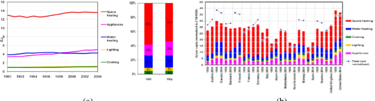
The major part of energy used in residential buildings is due to ‘Space heating’ as shown on Figure 4 (a). Differences can be observed between different countries, especially in terms of total (not normalized) energy use.
(a) (b)
Figure 4 : Subdivision of energy consumption in residential buildings in different countries (IEA (2008))
11
Energy consumption due to appliances is rising since 1990. This fact can be partly explained by the growing use of electrical equipment in residential buildings (computer, cell chargers, washing machine…). In 2004, the third source of energy used concerns the domestic hot water supply. Energy dedicated to lighting and cooking stays relatively stable and represents a smaller part of energy consumption (less than 10%).
This end-of-study project only focuses on the ‘Space heating’ and ‘Water heating’ energy reduction. Energy dedicated to these two sectors represents the major part of the residential used energy (more than 70%).
Moreover, cooking, lighting and appliances energy consumption highly depends on the electrical devices efficiencies and the human behavior (switching off lights, computer…). 1.4 Studied region
The present work focuses on the residential building situated in the Walloon Region of Belgium but this study could have been extended to another country by applying the same methodology.
The choice to focus only on the Walloon Region can be justified by this main fact: there are different energetic incentive policies (principally in terms of subsidy) between the North and the South of the Kingdom of Belgium. Moreover, many differences exist between the Flemish and the Walloon building stock in terms of year of construction and type of buildings (see Figure 9).
1.5 Research topic in the field of building sector: a short overview
As previously mentioned, many efforts are deployed in order to reduce our consumption in the (tertiary and residential) building sector. Several (International, European and Belgian) research projects have been, and are still, carried out to reach this goal. Examples are numerous. Here are some of the research projects carried out by the ‘Applied Thermodynamics Laboratory of the University of Liege’ which is very active in the energy domain:
- The ‘Appendix 53’ project consists in the development of analysis and evaluation procedures for total energy used in buildings;
- The ‘Harmonac’ project consists in the development of benchmarking, inspection and audit procedure for air-conditioned buildings. An aim of this project was to propose and evaluate some Energy Conservation Opportunities (ECO’s);
- The ‘Green +’ project consists in the development of an air-to-air heat recovery system for residential buildings;
- …
The whole description of these projects (and many others!) in the field of energy performance of building can be found on the website1 of the ‘Applied thermodynamics of the University the Liege’.
1
12
2 Statistic data on residential buildings situated in the Walloon Region of Belgium and Belgian energetic market
The present chapter focuses on the Walloon building census (typology, year of construction…), the Belgian energetic market (governmental Subsidies, oil and fuel price…) and the economical hypotheses used for the economical analysis.
2.1 Statistic data on residential buildings
The most recent national census related to residential buildings dates from 2001 and was performed by Vanneste et Al. (2001). Others used sources are the survey concerning the Walloon residential consumption carried out by the ICEDD (2005) and the investigation on the Walloon residential building stock performed by the MRW (2006-2007).
In the frame of the IEA-37 project (2006), a study (mainly based on the data presented in the three previously mentioned surveys) was managed by Kints (2008). The main part of the following results is extracted from this report.
2.1.1 Building Stock and Population
Wallonia’s total area is 16844km2 (29.5% of forest, 52.6% of cultivated area and 13.6% of urban zone). The total number of houses is equal to +/- 1 490 000 (+ secondary building). The total amount of people who live in Wallonia is 3 456 775 and the total amount of active people (15 to 64 years old) is equal to +/- 1 390 000. Density of population stands at 205.2 people per km2.
2.1.2 Buildings Type
Residential buildings can be classified in four categories: - 4 Frontages houses,
- Semi-detached houses, - Row houses,
- Flats.
2.1.3 Buildings Size
The buildings can be classified according to size, as shown on the Figure 6. This factor is important since the consumption dedicated to heating is proportional to the size of buildings.
13
Figure 6 : Buildings size distribution in the Walloon Region (Kints(2008)) 2.1.4 Correlation between sizes and types of buildings
Obviously, size and types of the building are highly correlated. On average, the number of rooms per residential building is 3.7 rooms per flat and 5.3 rooms per house. As expected, small flats (<55m2) are twice more numerous than small houses (< 55 m2).
Figure 7 : Correlation between sizes and types of buildings in the Walloon Region (Kints(2008))
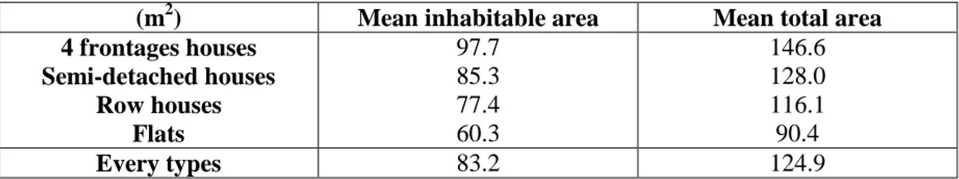
From these results, it is possible to determine the mean area per types of buildings. Results are given in Table 1:
(m2) Mean inhabitable area Mean total area
4 frontages houses Semi-detached houses Row houses Flats 97.7 85.3 77.4 60.3 146.6 128.0 116.1 90.4 Every types 83.2 124.9
Table 1 : Mean area according to types of building in the Walloon Region (Kints (2008))
2.1.5 Year of construction
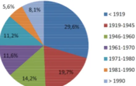
Year of construction is a primordial factor in our study since it is highly correlated with the insulation and the air tightness of the buildings. The global distribution of buildings according to their year of construction in the Walloon Region is given in the Figure 8:
14
Figure 8 : Global distribution of buildings according to their year of construction in the Walloon Region (Kints (2008))
As shown in the Figure 8, the Walloon housing stock is globally old: half of the residential building stock dates before 1945 and 75% dates before 1980. By assuming the fact that the buildings constructed before 1990 need a retrofit, 91.9% of the global stock is concerned. From this point of view, difference between the Flemish and the Walloon building stock is quite important, as shown in the Figure 9 :
Figure 9 : Spatial variation of the construction year of the building stock in Belgium Such differences can be explained by:
- a higher population density in Flanders; - a higher purchasing power in Flanders;
- a different socio-economic history between these two regions (industrial area in Wallonia);
- an interest for ancient buildings in Wallonia;
- a larger destruction of the buildings stock during the two world wars in Flanders;
- …
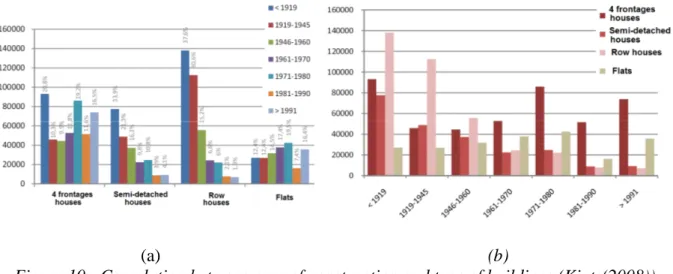
2.1.6 Correlation between year of construction and types of buildings
15
(a) (b)
Figure 10 : Correlation between year of construction and type of buildings (Kints(2008))
2.1.7 Constructive building stock characteristics
This part of the work describes the constructive characteristics of the Walloon building stock and focuses mainly on the wall, the roof and the window insulation.
Wall insulation
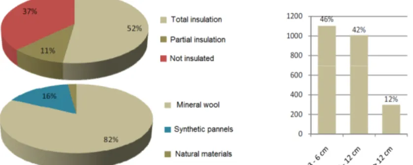
As we can observe on Figure 11, the main part (71%) of the residential building in the Walloon region is not totally insulated, which represents a high potential of amelioration.
Figure 11 : Insulation of the exterior walls: percentage of houses with insulation, type of insulation and insulation thickness (Kints (2008))
Obviously, a correlation between year of construction and degree of insulation exists. This correlation is represented hereafter, in
Figure 12.
16
Figure 12: Correlation between year of construction and degree of insulation
Unfortunately, statistic data about the correlation between the degrees of insulation and the type of building do not exist. In our study, we assume the same proportional repartition of the degree of insulation whatever the different type of building.
Roof insulation
There is a larger part (52%) of the roof insulated building stock compared to the exterior wall insulated building stock. However, almost 50% of the total building stock is not completely insulated, which also represent a high potential of amelioration.
Figure 13: Insulation of the roof: percentage of houses with insulation, type of insulation and insulation thickness (Kints (2008))
Unfortunately, correlation between year of construction and roof insulation are not available.
Windows
Figure 14 represents the part of insulated windows in the residential building stock of the Walloon region.
17
Figure 14 : Type of windows (Kints (2008))
Floor
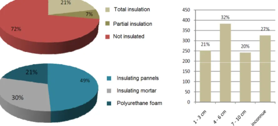
Floor insulation also represents a high potential of amelioration due to the high number of non-insulated residential buildings, as we can observe on Figure 15:
Figure 15: Floor insulation: percentage of houses with insulation, type of insulation and insulation thickness (Kints (2008))
Example of U value
Determining a mean value of the convective coefficient for all types of building is really difficult. To have an order of magnitude of U values of the existing building stock, examples of values measured on-site from real cases (in the frame of IEA 37 project), are given hereafter. One of the parts of this international project was to evaluate the energetic performance of residential houses before and after retrofitting (transforming into passive house).
18 Year of construction Type of building U_wall [W/m2K] U_roof [W/m2K] U_window [W/m2K] U_floor [W/m2K] BR AR BR AR BR AR BR AR Case 1 19th century Row house 3.14 0.135 5.5 0.14 4.65 0.72 2.2 0.165 Case 2 Beginning of the 20th Farm 3.14 0.26 0.76 (attic floor) 0.18 4.5 1.1 2.2 0.35 Case 3 50’s Semi-detached house 1.9 0.126 5.5 0.12 5 0.74 2.7 0.086 Case 4 1959 Social housing tower 2.78 0.41 0.77 (attic floor) 0.28 5.1 1.19 6.66 0.26 Case 5 1960 Single-detached house 2.12 0.2 3 0.21 2.6 1.1 3.65 0.49 *BR: Before retrofit *AB: After retrofit
As we can observe in the previous table, it is very complex to establish a correlation between the year of construction, the type and the U value of the construction. Correlation between U values used for our simulation and year of construction is presented in the chapter relative to the annual consumption simulation of the existing building stock.
2.1.8 Air tightness
One important factor to determine the annual energy consumption is the air tightness. Unfortunately, statistic data in relation with ages or building types about air tightness are difficult to find. A mean observed value of 12 [m3/h-m2] was chosen for non-retrofitted houses. This value is given by Renard (2008).
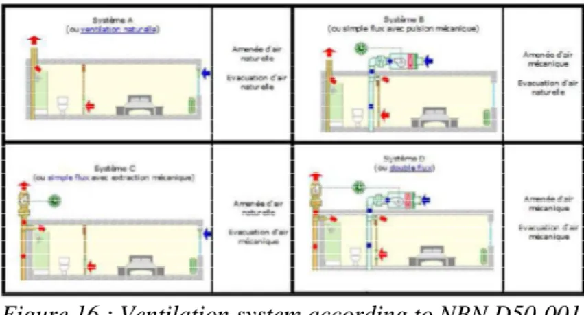
2.1.9 Ventilation
Residential ventilation can be divided into four categories: - System A : natural ventilation;
- System B: mechanic pulsing ventilation; - System C: mechanic extracting ventilation;
19
Figure 16 : Ventilation system according to NBN D50-001
In reality, detailed statistic data about ventilation system are not available in Walloon Region but it is a well known fact that the most widespread system is the system A (no mechanical ventilation) in non-retrofitted existing buildings. For our simulations, we consider this fact as an assumption.
2.1.10 Heating production system
This part of the work consists in presenting statistic data about the heating production system:
Figure 17 : Distribution of the building stock as a function of the heating production system (Kints (2008))
As we can see in Figure 17, Kints (2008) does not make difference between row houses, semi-detached houses and four frontages houses. In this end-of-study work, the distribution presented in Figure 17 is assumed to be equal for all types of houses. This remark can also be enounced for the following figure, which presents the distribution of the type of used combustible:
20
Figure 18 : Combustible used for space heating
70% of single-family houses and 76% of the flats are equipped with centralized heating production system. In both cases, gasoil and natural gas represent the main part of the energetic vector used:
- 68% of gasoil in single-family houses;
- 53% of natural gas and 41% of gasoil in flats.
Concerning decentralized heating production systems, natural gas and gasoil are less widespread than in centralized heating production systems. They represent 68% of the heating production system in the single-family houses, before electricity (12%), coal (10%) and wood (7%).
Electricity represents 30% of the combustible used in the decentralized heating production systems in flats.
There is a correlation between combustible used and year of construction, as we can observe on the following figure:
Figure 19 : Correlation between year of construction and type of combustible for space heating (Kints (2008))
2.1.11 Domestic hot water
As we can see on Figure 20, the production of domestic hot water is the second consuming use sector (11% of the total energy use), just after the space heating (74% of the total energy use):
21
Figure 20 : Distribution of the building consumption as a function of the type of use (Kints (2008))
Lighting is included in the electro part of the building consumption and represents 14% of this part. An easy way (maybe the easiest!) to reduce our environmental impact is to replace traditional lighting by low consumption (such as led) lighting. This solution will not be investigated in this end-of-study work.
Domestic hot water is mainly provided by electricity, natural gas and gasoil (in respectively 34%, 33% and 24% of investigated cases).
2.1.12 Assumptions concerning the determination of the envelope area
One important criterion in the determination of the building consumption is the heat loss area (and thus, the compactness of the building). Unfortunately, available statistic data about building area only concern the inhabitable and the total area (see 2.1.3).
Assumptions concerning the shape of the building have to be done in order to achieve the present study. The following part describes and justifies hypotheses used for each type of investigated residential building.
Figure 21 represents a schematic residential building and shows the nomenclature used in the rest of the paragraph:
- α is the slope of the roof; - y is the height of a storey;
- x is the length of the side frontage; - z is the length of the “street” frontage.
22
Figure 21 : Schematic representation of a residential building and used nomenclature
4 frontages houses
Concerning the 4 frontages houses, the first assumption is to consider the ground floor as a square (x=y). This fact can be justified by the observation of a sky view of a 4 frontages houses living district (Figure 22). The number of floor is equal to 3 (the ground floor, the first floor and the second floor also called the “under roof” floor) and the height of a storey (y) is chosen equal to 2.6 m.
Figure 22 : Sky view of a 4 frontages houses living district (Beaufays)
The rest of the assumptions are the same than the ones presented by Servais (2010): - α, the slope of the roof, is chosen equal to 25°C;
- the last floor of the building is supposed to be inhabitable when the height is comprised between 1.5 and 3m;
- the “street” frontage is composed of 30% of glazed area; - the “back” frontage is composed of 40% of glazed area; - the “side” frontages are composed of 30% of glazed area;
23 Semi-detached and row houses
Concerning the semi-detached and the row houses, it is established that the “street” frontage length is equal to 6 m. Once again, this fact can be justified by the observation of a sky view of row houses living district (see Figure 23).
Figure 23 : Sky view of rows houses living district (Grivegnée)
The rest of the assumptions relative to these two kinds of residential buildings are the same than the ones previously mentioned. One exception concerns the “under roof” floor. This latter is not supposed to be inhabitable, according to Servais (2010).
Flats
Obviously, α is equal to 0 and just one floor is considered. This latter is considered as a square. An example of apartment building is given in Figure 24.
Figure 24 : Apartment building (Liege: St Gilles) Assumptions relative to the percentage of glazed area are given hereafter:
- the “street” frontage is composed of 60% of glazed area; - the “back” frontage is composed of 40% of glazed area;
These values have been measured in a typical apartment from Liege (Quai Churchill, 11a). The rest of the assumptions are the same than the ones previously presented:
- the height of a storey is equal to 2.6 m;
- the apartment building is positioned in a way that it faces the “street” frontage to the east.
24
2.1.13 Determination of the envelope area and the volume
Thanks to the previously mentioned hypotheses (and the mean inhabitable area presented in 2.1.3), it is possible to determine the envelope area of each type of building by means of a set of simple equations (use of EES Software for calculus). Calculation details are given hereafter for each type of buildings.
4 Frontages house
In order to introduce the nomenclature used for our calculus, Figure 25 presents a schematic representation of a 4 frontage houses:
Figure 25 : Schematic representation of a 4 frontages house and its nomenclature (1) (2) (3) (4) (5) (6) (7) (8) (9) (10) (11) (12) (13) x4,front = z4,front y4,front = 2.6 l12 + 1.52 = l1 cos ( 25 ) 2 x4,front = 2 · l1 + l2
l2 · z4,front + 2 · x4,front · z4,front = 146.6
Atotal,roof,4,front = 2 · z4,front ·
x4,front
2 cos ( 25 )
Awall,street,4,front = 2 · z4,front · y4,front – Awind,street,4,front
Awind,street,4,front = 0.3 · 2 · z4,front · y4,front
Awall,back,4,front = 2 · z4,front · y4,front – Awind,back,4,front
Awind,back,4,front = 0.4 · 2 · z4,front · y4,front
Awall,side,4,front = 2 · x4,front · y4,front – Awind,side,4,front
Awind,side,4,front = 0.4 · 2 · x4,front · y4,front
25 (14) (15) (16) (17) (18) Semi-detached house
The same method that the one presented for the 4 frontage houses is applied. One of the difference concerns the determination of the total exterior area due to a common wall between the two attached buildings. Another difference is the fact that the under roof level is considered as uninhabitable. (19) (20) (21) (22) (23) (24) (25) (26) (27) (28) (29) (30) (31) (32) (33) (34) Row house
Same method is applied than the two previously presented:
(35) (36)
Atot,wind,side,4,front = 2 · Awind,side,4,front
Atot,ext,wall,4,front = Atot,wall,side,4,front + Awall,street,4,front + Awall,back,4,front Atot,wind,4,front = Atot,wind,side,4,front + Awind,street,4,front + Awind,back,4,front
h4,front2 + x4,front 2 2 = x4,front 2 · cos ( 25 ) 2
Vol4,front = x4,front · 2 · y4,front · z4,front +
x4,front 2 · z4,front · h4,front – l1 · 1.5 ySDH = 2.6 zSDH = 6 2 · xSDH · zSDH = 128 Atotal,roof,SDH = 2 · zSDH · xSDH 2 cos ( 25 ) Awall,street,SDH = 2 · zSDH · ySDH – Awind,street,SDH Awind,street,SDH = 0.3 · 2 · zSDH · ySDH Awall,back,SDH = 2 · zSDH · ySDH – Awind,back,SDH Awind,back,SDH = 0.4 · 2 · zSDH · ySDH Awall,side,SDH = 2 · xSDH · ySDH – Awind,side,SDH Awind,side,SDH = 0.4 · 2 · xSDH · ySDH Atot,wall,side,SDH = 1 · Awall,side,SDH Atot,wind,side,SDH = 1 · Awind,side,SDH
Atot,ext,wall,SDH = Atot,wall,side,SDH + Awall,street,SDH + Awall,back,SDH Atot,wind,SDH = Atot,wind,side,SDH + Awind,street,SDH + Awind,back,SDH
hSDH2 + xSDH 2 2 = xSDH 2 · cos ( 25 ) 2 VolSDH = xSDH · 2 · ySDH · zSDH + xSDH 2 · zSDH · hSDH yRH = 2.6 zRH = 6
26 (37) (38) (39) (40) (41) (42) (43) (44) (45) (46) (47) (48) (49) (50) Apartment
Apartments are the easiest type of building to determine the envelope area, since it is considered as a simple parallelepiped:
(51) (52) (53) (54) (55) (56) (57) (58) (59) (60) (61) (62) (63) (64) (65) Values resulting from the set of equations are given hereafter. These are the ones that we will use for our simulations:
2 · xRH · zRH = 116.1
Atotal,roof,RH = 2 · zRH · xRH
2
cos ( 25 )
Awall,s treet,RH = 2 · zRH · yRH – Awind,s treet,RH
Awind,s treet,RH = 0.3 · 2 · zRH · yRH Awall,back,RH = 2 · zRH · yRH – Awind,back,RH Awind,back,RH = 0.4 · 2 · zRH · yRH Awall,side,RH = 0 Awind,side,RH = 0 Atot,wall,s ide,RH = 0 Atot,wind,s ide,RH = 0
Atot,ext,wall,RH = Atot,wall,s ide,RH + Awall,s treet,RH + Awall,back,RH
Atot,wind,RH = Atot,wind,s ide,RH + Awind,s treet,RH + Awind,back,RH hRH2 + xRH 2 2 = xRH 2 · cos ( 25 ) 2 VolRH = xRH · 2 · yRH · zRH + xRH 2 · zRH · hRH zflat · xflat = 90.4 zflat = xflat yflat = 2.6 Atotal,roof,flat = 0
Awall,street,flat = xflat · yflat – Awind,street,flat
Awind,street,flat = 0.6 · xflat · yflat
Awall,back,flat = zflat · yflat – Awind,back,flat Awind,back,flat = 0.4 · zflat · yflat
Awall,side,flat = 0 Awind,s ide,flat = 0 Atot,wall,s ide,flat = 0 Atot,wind,s ide,flat = 0
Atot,ext,wall,flat = Atot,wall,s ide,flat + Awall,street,flat + Awall,back,flat
Atot,wind,flat = Atot,wind,s ide,flat + Awind,s treet,flat + Awind,back,flat
27
28
3 Walloon residential building stock arborescence
This part of the work is the most delicate one. Actually, it is really difficult (and even impossible) to create an arborescence of the different kind of residential buildings situated in the Walloon Region: purists would say that there are as many cases as there are buildings! It also exists a compromise between a large numbers of investigated cases (to be as complete as possible and to analyze as many cases as possible) and a small numbers of analyzed cases (to be as efficient as possible in terms of calculating time). In order to reduce the case number, the idea is to neglect marginal cases.
Moreover, the creation of the building stock arborescence requires a large numbers of assumptions. Error sources are also abundant: statistics and data compilation, used assumptions, used weather data…
In conclusion of this chapter’s introduction, it is important to keep in mind that the presented method does not permit to determine with precision the global consumption of residential buildings in the Walloon Region. On the other hand, this latter method allows pointing out some economical and environmental trends related to the different investigated retrofit options.
3.1 Determination of the existing building stock arborescence
As already mentioned, a compromise exists between a large numbers of investigated cases and a small numbers of analyzed cases. In a first time, a large arborescence with a maximum of investigated cases will be created; then simplifications will be made in order to reduce the number of cases.
3.1.1 Large arborescence
The creation of the largest building stock arborescence can be made by investigating all possible cases from the statistic data previously presented.
Large building stock arborescence
Type of building
(Separated, Semi-detached and Row houses + Apartment)
4
Area
(Small, Medium, Large and Very large)
4 Year of construction (<1919, 1919-1945, 1946-1960, 1961-1970, 1971-1980, 1981-1990, >1990) 7 Wall
(Insulated, Partially insulated, Not insulated)
3
Roof
(Insulated, Partially insulated, Not insulated)
3
Window (Insulated, Not insulated)
2
Floor
(Insulated, Partially insulated, Not insulated)
3
Heating production system (Centralized, Not centralized)
2
Type of combustible
(Gasoil, Natural gas, Electricity, Wood, Butane/Propane, Coal, Others)
7
DHW
(Gasoil, Natural gas, Electricity)
3
Total number of cases 190 512
29 3.1.2 Simplified arborescence
First step
As we can observed in the previous paragraph, the large building stock arborescence presents 190 512 of investigated cases, which is way too high in the field of this study. Simplifications have to be done.
3.1.2.1.1 Simplification concerning the type of building and the inhabitable area
It has been decided to correlate the type of building and the inhabitable area, by using the mean value presented in Table 1. So, a mean inhabitable area corresponds to a type of building. This simplification divides the number of investigated cases by 3.
3.1.2.1.2 Simplification concerning the year of construction
Year of construction is divided into seven parts rewritten henceforward:
- <1919, 1919-1945, 1946-1960, 1961-1970, 1971-1980, 1981-1990, >1990.
Simplification consists in aggregating the first and second group, the third and fourth group and lastly the fifth and sixth group.
Year of construction is now classified as presented hereafter: - <1919-1945, 1946-1970, 1971-1990, >1990.
This simplification can be justified by the observation of Figure 10 and Figure 12 which shows the same trends of characteristics for each aggregated groups.
3.1.2.1.3 Simplification concerning wall, roof and floor characteristics
Simplifications concerning the wall, roof and floor characteristics consist in neglecting the partially insulated case, which is quite negligible. Parts relative to the partially insulated case are proportionally split up.
3.1.2.1.4 Simplification concerning the heating production system
No simplifications can be made concerning the heating production system.
3.1.2.1.5 Simplification concerning combustible and domestic hot water (DHW)
Simplification concerning the combustible and the domestic hot water is to focus only on the main used combustible: gasoil, natural gas and electricity. Moreover, another simplification consists in assuming that production of domestic hot water can be done only by the same type of combustible than the one used for the space heating or by electricity.
30
3.1.2.1.6 Determination of the total number of investigated cases
Simplified building stock arborescence
Type of building correlated with mean inhabitable area
(Separated, Semi-detached and Row houses + Apartment)
4
Year of construction
(<1919-1945, 1946-1970, 1971-1990, >1990) 4
Wall
(Insulated, Not insulated) 2
Roof
(Insulated, Not insulated)
2
Window (Insulated, Not insulated)
2
Floor
(Insulated, Not insulated)
2
Heating production system (Centralized, Not centralized)
2
Type of combustible and DHW
(Gasoil + Gasoil, Natural gas + Natural gas, Gasoil + Electricity, Natural gas + Electricity, Electricity +
Electricity)
5
Total number of cases 2560
Table 3 : Simplified building stock arborescence (First step)
Second step
As we can observe in Table 3, the total number of cases from the first simplified arborescence is equal to 2560 which is too numerous in the frame of this study. Thus, it has been decided to reduce this number by making more simplifications:
- The first simplification consists in neglecting the insulation of the floor. A mean value will be used for our simulation. This can be justified by the fact that most of the basement floor is situated above a technical local or a cellar which reduce the influence of the floor insulation. Moreover, retrofit options relative to the floor insulation are not widespread (heavy building work).
- It has also been decided not to take into account the type of heating production (centralized or decentralized) but only the energetic vector. This simplification can be justified by a weak influence of the heating production system in the annual consumption. In our study, we will only consider a centralized system for two reasons. It is the most widespread system and retrofit options are mostly centralized ones.
- Obviously, roof insulation is not taken into account in the flat simulation (roof of an apartment is not an “exterior” wall).
- Since the walls are not the easiest component to insulate and if the walls are insulated, it has been decided to consider the roof and the windows as also insulated (if the owners have decided to insulate their walls, they have probably/certainly made the efforts to insulate their roof and their windows).
31
- Windows (even if the wall is not insulated) are considered as insulated for building constructed after 1990.
3.1.3 Repartition hypotheses
Some of the simplifications presented in the previous paragraph (and more precisely the two last ones) can be justifiably considered as repartition hypotheses.
In reality, statistic data about Walloon residential building stock presented in the Chapter 2 does not permit to generate a complete arborescence. The creation of this latter requires the use of some repartition hypotheses. For example, no correlation exists between windows insulation and year of construction of the building (or between windows insulation and type of building).
Thus, as already mentioned, it has been decided to consider windows from building constructed after 1990 as insulated. For building constructed between 1946 and 1970 or between 1970 and 1990, repartition is the same than the one presented in Figure 14 (19.1% insulated vs 80.9% not insulated). In order to reach the same repartition as the one presented in Figure 14 for a type of building, repartition for windows from building constructed before 1945 is adapted (an Excel file was created to generate the arborescence).
Concerning the repartition of the roof insulation, the same problem that the one met with the windows insulation can be enounced: correlation between year of construction and/or type does not exist. The same method that the one presented in the case of the windows insulation is applied. Roof of building constructed after 1990 are considered as insulated. Another hypothesis is to consider as not insulated, roofs from building with windows and walls not insulated. Percentages of insulated roofs constructed between 1970 and 1990 and between 1946 and 1970 are respectively equal to 80%. In order to reach the same repartition as the one presented in Figure 13 for a type of building, repartition for roofs from building constructed before 1945 is adapted (in view of the previous hypotheses and repartition presented in Figure 13, it is obvious that most of the non insulated roofs comes from building constructed before 1945).
All of these previously presented simplifications/repartition hypotheses allow reducing the number of investigated cases to 265 which is considered as satisfactory for this study. An example of 20 cases resulting from the arborescence is given hereafter, in Figure 26. The whole arborescence is given in Appendix D.
32
Figure 26 : Building stock arborescence
3.2 Arborescence: some interesting numbers
Some interesting numbers can be stressed by creating the Walloon building stock arborescence.
Among them and as an example, the most represented building (2.8% of the building stock) is a row house constructed with not insulated walls, insulated windows and roofs, and natural gas as an energetic vector (for both heating space and domestic hot water). The less represented one (negligible part of the building stock) is a row house constructed between 1971 and 1990 with not insulated walls and roofs, and insulated windows with natural gas for space heating and electricity for domestic hot water.
33 4 Envisioned Retrofit Options
In the field of residential building, a high number of retrofit options can be investigated. As already mentioned in paragraph 2.1.11, replacement of traditional light by diodes is a good way (and maybe the easiest) to reduce our consumption.
In the frame of this end-of-study project, envisioned retrofit options concern only envelope insulation and heating/electricity production system improvement.
More precisely, our study focuses on: - walls, roof and windows insulation;
- replacement of the current heating production system by a condensing boiler or an heat pump. Investigations about solar panels will also be carried out.
We may extend this list of retrofit options, but it has been chosen to investigate the most widespread ones in the frame of this end-of-study work. As an example, we could investigate photovoltaic panel but this latter does not match to the frame our subject which concern energy consumption reduction relative to building. In this context, photovoltaic panels can be considered as a system of electricity production and investigated as such.
This section briefly presents some of the retrofit options investigated in this end-of-study work.
4.1 Insulation
There are several methods of wall insulation. We can classify them into 3 categories: - “inside” wall insulation (a);
- “outside” wall insulation (b), - “by cavity” wall insulation (c).
Examples of the three types of retrofit insulation are given in Figure 27:
(a) (b) (c)
Figure 27 : Types of wall insulation
4.2 Condensing boiler
A condensing boiler utilizes the latent heat of water produced from the burning of gasoil or natural gas, in addition to the standard sensible heat, to increase its efficiency.
34
Figure 28 : Schematic representation of a condensing boiler (Makaire et al. (2010)) To take advantage of this technology, the supply water temperature has to be inferior to the dew-point temperature of the flue gas. As we can observe in Figure 29, the supply water temperature highly influences condensing boiler performance.
Figure 29 : Measured condensing boiler performances (Makaire et al. (2010))
From this fact, it is important to keep in mind that the emission system has to be designed to reach a supply temperature as low as possible.
4.3 Heat pump
According to Ashrae (2004), a heat pump is a machine or device that diverts heat from one location (the 'source') at a lower temperature to another location (the 'sink' or 'heat sink') at a higher temperature using mechanical work or a high-temperature heat source.
A heat pump is made of 4 main components:
- A compressor: its role is to raise the pressure of the refrigerant by means of a mechanical work. It operates thanks to an electrical motor.
- A condenser: is a heat exchanger. Its role is is to allow the condensation (passage from the vaporous state to a liquid state) of the refrigerant. This latter release an amount of heat to a secondary fluid.
- An expansion valve: its role is to decrease the pressure of the refrigerant.
- An evaporator: is also a heat exchanger. Its role is to evaporate the refrigerant by allowing the absorption of an amount of heat from a secondary fluid.
35
Figure 30 : Schematic representation of a heat pump
The P-h evolution of a refrigeration cycle is given hereafter:
Figure 31 : P-h diagram of a heat pump cycle2
A four-ways valve can be added to the previous list of heat pump components. This component allows the reversibility of the cycle.
Heat pump performances are characterized by their Coefficient Of Performance (COP) when the device working in heat pump mode, or by their Energy Efficiency Ratio when the machine working in chiller mode.
COP and EER are defined by the two following equations: ܥܱܲ =ܳሶௗ
ܹሶ ܧܧܴ =ܳሶܹሶ௩ 4.4 Solar panels
Solar panels, also known as solar collectors, are placed on the roofs of buildings, oriented as much as possible towards the south. They receive heat from the sun and transmit it to an antifreeze fluid that circulates inside. This fluid goes through insulated pipes to a storage tank.
2 Source : http://www.refrigerationbasics.com Condenser Evaporator Compressor Expansion valve
36
This storage tank can be used to provide domestic hot water, or contribute to the central heating system. They are usually coupled to a conventional boiler in order to provide heat demand in every condition.
An example and schematic representation of the system is given in Figure 32:
Figure 32 : Basic principle of thermal panels3
3
37
5 Simulated annual consumption for existing building stock 5.1 CALE
Several existing software such as Opti-maison (Architecture et climat, 1998) or SISAL (which means in French “SImulation de Systèmes Accessibles en Ligne”) are available to carry out this kind of study. It has been decided to choose the CALE (also called PEB which means in French “Performance Energetique des Bâtiments”) Software for its easiness of use and also mainly for its small calculation time (less than one second) compared to SISAL Software (more or less one hour). SISAL Software is more precise (hourly-based dynamic simulation) than CALE Software (interpolation). This end-of-study work is based on many assumptions and, as already mentioned, these assumptions don’t lead to precise calculus. Considering this fact, it would be ridiculous to prefer a long-time simulation precise Software.
5.1.1 Description of the ‘CALE’ software
‘CALE’ software is a tool able to estimate the annual consumption (and the cost relative to the annual energy consumption) for residential buildings. The tool is mainly intended for engineering consulting firm, architects, components manufacturers and retailers. The CALE Sofware was developed on ‘Excel’.
The ‘residential’ (in opposition of ‘tertiary’) version obviously permits the analysis of all types of building:
- Single family houses, - Row houses,
- Semi-detached houses, - Flats.
5.1.2 Input data
Obviously, ‘CALE’ software requires a minimum number of inputs to run simulations: - Surface of walls, windows, doors, floor, roof;
- Thermal transmittance, (in W/m2K), is the rate of transfer of heat (in W) through one square meter of a structure divided by the difference in temperature across the structure. These values have to be specified for walls, windows, floor, roof…;
- Type of ventilation and the ventilation flow rate; - Presence or not of a heat recovery device; - Centralized or decentralized heating production;
- Type of heating production (heat pump, boiler, condensing boiler, …); - Type of emitters (radiators, heating floor,…);
- Type of heating production for domestic hot water; - Cost of energy (electricity, gas, annuity, etc…); - Air tightness;
- other inputs such as the number of sinks;
- …
An example of an input data sheet from the CALE Software is given in Figure 33. This input data sheet concerns the geometric characteristic and the degree of insulation of the building.
38
Figure 33 : Example of an input data sheet from the "CALE" Software
5.1.3 Weather data
Walloon climate is supposed to be equivalent from one Walloon geographical zone to another since the small area considered (16844 km2). The Software does not permit the modification of the weather data (contrary to “SISAL” Software by example).
5.1.4 Output data
CALE Software is able to produce the following outputs:
- Annual total consumption due to the space heating, the space cooling (almost always equal to zero in residential building), domestic water heating and auxiliaries;
- Total cost relative to the consumption mentioned in the previous point; - Total amount of final energy consumed;
- Total amount of primary energy consumed; - Total amount of CO2 produced per year.
39
Figure 34 : Results synthesis sheet from the CALE Software
5.1.5 Assumptions concerning simulations
Such as for the creation of the building stock arborescence, statistic data and/or correlations (with year of construction and/or type of building by instance) do not exist about U value or heating production system efficiency. Assumptions concerning these values have to be done in order to realize our study.
The first type of assumptions concerns U value. We consider a U value for windows, walls and roofs of respectively 4.65, 3.14 and 3.13 for non insulated buildings constructed before 1945. We consider an improvement of buildings efficiency over the years and thus, a reduction of 20% and 40% of the previously presented U value for buildings respectively constructed between 1946 and 1970 and buildings constructed after 1970.
Concerning insulated components (walls, roofs and windows), we use mean value measured in situ on new constructions. These values are given by Lagendries (2008).
40
The second type of assumptions concerns heating production system efficiency. Values of 77%, 85%, 87% and 89% have been chosen for buildings respectively constructed before 1945, between 1946 and 1970, between 1971 and 1990 and after 1990. A value of 85% has been chosen to characterize the emission system efficiency.
5.2 Validation of the developed method
The present part of the work consists in comparing results obtained from the exposed method and the actual building consumption.
According to Kints (2008), the mean average value for a residential house in term of total final energy is equal to 26.8 MWh. As shown in Figure 36, the part relative to the space heating is comprised between 75% and 78% of this total energy. The part relative to the domestic hot water is comprised between 10 and 12%. The mean annual consumption relative to space heating and domestic hot water in term of final energy is estimated (a top-down methodology is used: repartition of the total amount of consumed energy per sector) equal to 24120 MWh per year with 13.3% due to water heating (if we only consider these two energy vectors).
Figure 36 : Building consumption (DGSIE and ICEDD for the DGO4 (data from 2007)) Our simulations (total amount of 265) have permit to determine the annual consumption relative to domestic hot water and space heating for each type of building. These latter results have been average weighted by means of percentage of occurrence determined by the building stock arborescence. A mean annual consumption per Walloon residential building (in term of final energy) of 27558 kWh per year was found with 8.83% due to domestic hot water. It has been decided not to take into account ‘auxiliaries’ consumption (considered as domestic appliance). It has also been possible to determine the mean annual CO2 emission per house: 8.25 t/an.
Difference between official results and our results is less than 12.5% and difference between the repartition of domestic hot water is less than 5%.
Can we consider results from our simulations as satisfying and can we explain the difference between the two results?
In reality, differences between results from our calculation and official results can be explained by many reasons:
- Our method uses a high number of assumptions (geometric characteristics, evolution of U value over the year of construction, repartition assumptions, weather,… ),
- “Official” method (top-down methodology) also uses a high number of assumptions, - CALE Software overestimates annual consumption (practical comparison with
41
- Simulation-based consumption determination of a building is quite difficult (because of the influence of a high number of factors) and requires a calibration (adjustment of parameters of the model) to fit the reality. To have an order of magnitude, a comparison between actual consumption and simulation-based results as a function of the simulation runs (tertiary building) is given hereafter by Bertagnolio et al (2010) :
Figure 37 : Calibration vs simulation runs
Determination of the annual consumption of the building stock in term of final energy could be the object of a calibration by adjusting some of the parameters (such as U value or efficiency of heating production system) in order to fit the mean “official” consumption. As official method (top-down) also uses a high number of assumptions, it has been decided to not carry out this “calibration”.
In conclusion, we can consider results of our simulation as (very) satisfying. Moreover, as already mentioned, the aim of this study was not to determine with precision the mean consumption in the Walloon region, but to stress some trends resulting from a refurbishment.
5.3 Consumption vs type of building
Obviously, consumption is linked (among other things!) to the type of building. We can stress some trends relative to this latter fact. As an example, row houses consume less than 47% of energy compared to 4 frontages houses (average value). This can be justified by two major facts:
- Row houses are considered smaller (21.4 % in term of inhabitable area) than 4 frontages houses, in our simulations (146.6 vs 116.1 m2 of mean inhabitable area: see Table 1);
- “Exterior” walls area (and thus windows area) is obviously smaller for row houses than for 4 frontages houses.
We can compare our results with the ones given by Renard (2008): he shows that a row house consumes 36% less than a 4 frontage houses (by considering the same inhabitable area for both types). Our results are in the same order of magnitude than the ones presented by Renard (2008).
If we transform these results in annual consumption per square meter (normalized consumption), we can observe that row houses are 26% more efficient than 4 frontages houses.
Obviously, we can extend this analysis to semi-detached houses (which consumes 24.4% less than 4 frontages houses) and apartments (which consumes 76% less than 4 frontages houses).
42
Apartments are the type of building the most efficient in term of energy consumption. This can be justified by the two previously mentioned facts (smaller inhabitable area and smaller “exterior” wall area) and one supplementary: in our simulations, roof area is consider equal to zero.
This first observation of our simulation results is highly important and a major conclusion of this end-of-study work can already be enounced:
- type of residential construction highly influences energy consumption. Obviously, the ranking is the following one: the best type of building in terms of energy efficiency is the apartment type, the second one the row house type, the third one is the semi-detached house type and the worth one is the 4 frontages house type.
As we can observe in Figure 10, major part of the new construction (after 1991) concerns 4 frontages houses. Better information and/or incentive policies should be given to urge builder to opt for row house type than 4 frontage house type.
43 6 Economic analysis
One of the aims of this end-of-study project is to evaluate the economical potential of different (combination of) retrofit options.
The present chapter is divided into several parts. First, investment costs related to each retrofit option are investigated. Secondly, energy costs are detailed. The third part of the section investigates different economic methods. One of them is chosen in order to carry out the study and compare the investigated retrofit options.
The comparison of the retrofit options in terms of economic analysis will be done in section 8. 6.1.1 Investment costs
Investment cost relative to each investigated refurbishment option corresponds obviously to one of the most important factor in an economic study. Prices given in this end-of-study come from an interview of one of the founders of “Enersol” and from different websites45 dedicated to professionals in the building sector. A list of indicative prices of windows is given in Appendix E.
The boiler chosen for this end-of-study work is the boiler ALU DOMUS (KV 120 20 SAI) from the brand Riello. This boiler is suitable for heating only or for heating and DHW. It has an average power of 12.5 kW with performances of about 102-108%. The purchase price is € 3750.
Just as the boiler, the chosen heat pump comes from the brand RIELLO. The model can operate in SINTESY reversible air conditioning in summer. Rated power is 6.6 kW for a COP of 3.9. Its purchase price is € 5535.
Retrofit options Price
Wall insulation [€/m2]
40-60 for int. insulation 60-75 for ext. insulation
65- by insufflations Roof insulation [€/m2] 50 Windows [€/m2] 90 Condensing boiler [€] 3750 Heat pump [€] 5538 Thermal panels [€/m2] 1000-1200 6.1.2 Energy costs
This section presents the cost of energy depending on the energetic vector (fuel, electricity and gas).
Fuel cost
The mean price of the Belgian heating fuel is given by Statbel (2011):
4 http://www.livios.be/
5
44
Figure 38 : Mean fuel cost (Statbel, (2011))
Concerning our study, just one price is considered and corresponds to the mean average value of the four previous values exposed in the tab: 0.7212 €/liter.
Electricity cost
Since 2007, the Belgian electricity market is liberalized. The electricity cost depends on the supplier (their total number is fifteen according to the CREG which means in French “Commission de Régulation de l’Electricité et du Gaz”).
Actually, the electricity price is also dependant on the time schedule in the day. To be as precise as possible, it is important to notice that the total electricity price corresponds to the sum of several parts:
- Annual fixed fee and green contribution; - Energy cost;
- Electrical network use cost (distribution cost + transport cost); - Use tax, fee, contribution and excess load.
The repartition of the electricity price is important because the SISAL Software requires “Annual fixed fee” and “Electricity Cost for Night and Day” as inputs.
In order to have a control on the electricity price and to protect citizens against an eventual monopole, an organism called the CREG regulate the electricity market by fixing electricity price.
According to a major Belgian supplier (Luminus (2011)), the electricity cost disaggregation is given hereafter. The following prices take into account the value added taxes and consider a bi-hour electricity meter (the most widespread one). Concerning the electrical network use cost and the electricity meter renting, the presented price corresponds to the mean average of the prices of the several electrical network manager in the Walloon Region.
- Annual fixed fee = 117.53 [€/an]; - Day energy cost = 9.58 [c€/day kWh]; - Night energy cost = 5.91 [c€/night kWh]; - Green contribution = 1.06 [c€/kWh];
- Electrical network use cost = distribution cost + transport cost = 8.84 + 1.06 = 9.9 [c€/kWh];
- Electricity meter renting = 16.04 [€/an];
- Use tax, fee, contribution and excess load = 0.943[c€/kWh].
From these results, it is possible to disaggregate the electricity cost in three categories: - Annual fixed cost = Annual fixed fee + Electricity meter renting
= 117.53 + 16.04 = 133.57 [€/an];
- Day electricity cost = Day energy cost + Green contribution + Electrical network use cost + Use tax, fee, contribution and excess load = 9.58 + 1.06 + 9.9 + 0.943 = 21.48 [c€/day kWh]; - Night electricity cost = Night energy cost + Green contribution +