by
Matthew H. Burt
B.A., Japanese language and economics (1991) The Ohio State University
Submitted to the Engineering Systems Division in partial fulfillment of the requirements for the degree of
Master of Engineering in Logistics at the
Massachusetts Institute of Technology June 2000
@ 2000 Matthew H. Burt All rights reserved.
The author hereby grants to M.I.T. permission to reproduce and to distribute publicly paper and electronic copies of this thesis document in whole or in part.
Signature of Author
Engineering Systems Division May 5, 2000 Certified by Executive Director, Ma t Accepted by MASSACHUSETTS INSTITUTE OF TECHNOLOGY
JUN 01
2000
LIBRARIES James Masters of Engineer ng in Logistics Program Thesis SupervisorYossi Sheffi Director, Mastej4f Engineering in Logistics Program
An Algorithm to Determine the Causes of Inventory Stock-outs in Manufacturing Firms by
Matthew H. Burt
Submitted to the Engineering Systems Division on May 5, 2000 in partial fulfillment of the requirements for the degree of Master of Engineering in Logistics at the
Massachusetts Institute of Technology ABSTRACT
The recent trends in manufacturing toward lower inventory levels, shorter cycle times, and more closely integrated production schedules have led to an extremely low tolerance for inventory stock-outs. In such an environment, any shortage is costly, and
understanding why stock-outs occur and how to prevent them is an important issue. However, the answer to the question of why stock-outs occur is not always easy to determine. Investigations into the root causes of inventory stock-outs are often hindered by data collection problems, data overload, and the investigators' lack of a well-accepted,
systematic framework with which to conduct the analysis, resulting in a cursory review of the problem and a subjective diagnosis.
This thesis proposes an algorithm to determine objectively the causes of inventory stock-outs in manufacturing firms. Instead of observing stock-stock-outs through the lens of the classical inventory model that aggregates all variations in resupply time and demand during leadtime into one variable, this thesis attempts to view the problem with a broader supply chain perspective that considers multiple sources of variation. Given data that describe the transactions of materials and information between members of the supply chain, the algorithm identifies which causes among a prescribed set of causes lead to a given stock-out occurrence. The transaction data is analyzed using a simple supply chain model to determine how each possible stock-out cause could affect actual inventory performance compared to planned inventory performance.
This approach to analyzing inventory stock-outs has many possible uses, including its use as a supply chain metric to evaluate efforts to minimize inventory stock-outs.
Thesis Supervisor: James Masters
TABLE OF CONTENTS
1. INTRODUCTION ... 4
2. LITERATURE REVIEW ... 6
3. DEVELOPM ENT OF THE ALGORITHM ... 8
3.1 W HAT IS A STOCK-OUT? ... .. .. .. .. . .. .. .. . .. .. .. .. .. . .. .. .. . .. .. .. . .. .. . .. .. .. . .. .. . . .. 8
3.11 Definition of a Stock-out ... 9
3.12 Illustration of a Stock-out ... 9
3.13 Quantifying Stock-outs - A Definition of Stock-out Magnitude ... 10
3.2 W HAT CAUSES STOCK-OUTS?... . . .. .. .. .. . .. .. .. .. .. . .. .. .. . .. .. . .. .. .. . .. .. .. . .. .. .. . . 11
3.21 Variance Between Planned and Actual Inventory System Performance... 11
3.22 Safety Stock Levels as an Influence upon Stock-outs... 14
3.23 A Supply Chain Model... 15
3.231 Description of the Model ... 15
3.232 Simplification of the Model ... 17
3.233 Variations on the Model... 18
3.24 A Supply Chain Transaction Log... 19
3.241 Supply Chain Parameters ... 19
3.242 Supply Chain Transaction Data Elements ... 20
3.243 Graphical Representation of Transactions ... 24
3.244 Narration of Sample Transactions... 26
3.3 W HAT KINDS OF STOCK-OUT CAUSES EXIST?... 27
3.31 Two Dimensions of Stock-outs - Quantity and Time... 27
3.32 Classification Codes ... 29
3.4 HOW DO MULTIPLE STOCK-OUT CAUSES INTERACT? ... . .. .. . .. .. .. . .. .. . .. .. .. . .. .. .. . .. .. . . . .. 30
3.41 Methodology for Understanding Multiple Cause Interaction... 30
3.42 Overlapping Multiple Stock-out Causes ... 31
3.42 Accumulating and Compounding Multiple Stock-out Causes... 34
3.5 HOW TO IDENTIFY STOCK-OUTS?... . . .. .. .. .. .. . .. .. .. . .. .. .. . .. .. . .. .. .. . .. .. .. . .. .. . .. .. . 37
3.5 1 Sa m p le da ta ... 38
3.52 Test to Identify Quantity-based Stock-out Causes ... 41
3.53 Test to Identify Postponed Time-based Stock-out Causes... 42
3.54 Test to Identify Retarded Time-based Stock-out Causes... 44
3.6 HOW TO DETERMINE STOCK-OUT CAUSES - STATEMENT OF THE ALGORITHM... 45
3.7 EXPERT SYSTEM APPLICATION ... 46
4. IMPLEMENTATION ISSUES ... 47 4 .1 C A PA B ILITIE S ... 47 4 .2 D A TA N EED S ... 4 8 4 .3 S Y STEM D ESIG N ... 49 5. CONCLUSION ... 50 6. BIBLIOGRAPHY ... 52
1. INTRODUCTION
The recent trends in manufacturing toward lower inventory levels, shorter cycle times, and more closely integrated production schedules have led to an extremely low tolerance for inventory stock-outs. In such an environment, any shortage is costly, both in financial terms and in terms of a firm's reputation. Therefore, understanding why stock-outs occur and how to prevent them is an important issue for any organization. However, the answer to the question of why stock-outs occur is not always easy to determine.
Sometimes, a specific incident such as a late supplier delivery, a shut-down production line, or a spike in customer orders, may jump to mind as the cause of a specific problem. Sometimes, a combination of such incidents occurring at about the same time as the shortage will appear to be the answer. If the causes seem obvious, it may be reasonable for an inventory manager to move on to designing some corrective action to prevent a recurrence.
Other times, however, the cause may not be as salient, and a closer analysis may be required. In this case, it may be difficult to review the facts leading up to the stock-out. The necessary data to determine stock-out causes may be located in the internal reports of several departments and span several time periods. Even assuming the appropriate reports could be collected, interpreting them might require significant knowledge about the procedures followed by the many different actors in the inventory system. Without a systematic way to analyze the data, it might be tempting to simply scan the data until
some instance of glaringly aberrant data appeared that would seem to explain the occurrence of the inventory stock-out.
This haphazard sort of analysis raises several questions. How does one know when enough data has been collected? How does one ensure that all data are being evaluated fairly? How can one simplify the method of collecting and evaluating the data? This thesis will attempt to answer these three questions by developing an algorithm to determine the causes for inventory stock-outs.
First, in Section 2 of the thesis, a literature review will cover the relevant concepts needed to develop the algorithm. Next, Section 3 will describe the development of the algorithm itself. Section 3.1 will open this development by exploring how to define and quantify inventory stock-outs. Section 3.2 will then consider the classical inventory model of stock-outs and introduce a simple supply chain model with a transaction log. Section 3.3 will classify stock-out causes along two dimensions. Section 3.4 will explore how
multiple stock-out causes interact. Lastly, Section 3.5 will describe a simple expert system that uses elements of the classical inventory model, the supply chain model, and the transaction log which forms the basis of the algorithm of this thesis. After developing the algorithm, Section 4 will outline implementation issues including capabilities, data needs and system design; and Section 5 will offer a conclusion.
2. LITERATURE REVIEW
The specific problem described in the introduction has not been treated directly in the existing literature on inventory theory. However, several fundamental concepts found in inventory theory, expert system design, and cost accounting are helpful in building a framework with which to address the issue.
The starting point for most discussions of inventory is the classical sawtooth inventory model which has been summarized by Tersine (1988). This model is used to describe how inventory levels fluctuate as inventory is received and consumed. It is also used to explain the concepts of a stock-out, cycle stock and safety stock, backordering, and how all stock-outs are the result of some variation in product supply, demand, or a
combination of both.
Traditionally, variations in resupply time and demand during lead time have been modeled as an aggregate lead time variance. This allows for mathematical inventory models that can be used to determine appropriate safety stock levels and estimate the costs of an inventory system. In practice, however, the resupply time and demand during lead time of a product are separate events, even though they may be influenced by each other. Ballou (1992) describes how these two components of lead time variance, which are measurable in practice, can be aggregated for purpose of simplification in modeling.
Most treatments of inventory theory simply define a stock-out as an instance of available inventory levels not meeting customer demand. Bernard (1999) makes a further
distinction between stock-outs and "out-of-stock" conditions, the latter referring to times when there is zero demand and a firm plans to have no inventory.
This paper introduces a method for quantifying the magnitude of a stock-out occurrence and assigning portions of its magnitude to one or more causes. The concept of measuring the actual performance of a system and comparing it to a standard is also found in cost accounting (Refer to Polimeni, 1991 for a summary.). One branch of this field, known as variance analysis, defines how the variance between actual and standard performance of system can be mathematically attributed to one or more causes. This paper uses the concepts of variance analysis in building a framework to understand stock-outs.
Although a stock-out may be easily detected and measured using the concepts described above, actually determining which among a certain set of causes were the source of the stock-out can be achieved using the forward chaining logic found in expert systems. Giarratano (1998) offers a summary of this logic, and Efstathiou (1992) provides an excellent example of how it applies to manufacturing systems. Many examples of expert systems designed for different aspects of inventory systems exist, of which Carlson (1996) and Ehrenberg (1990) are just two examples. However, a search for systems that specifically treat the question of how to assign causes to stock-outs yielded none
discussed in academic literature.
It is very likely that some firms have built in-house information systems to determine the causes of stock-outs, but such systems are not common in industry today. Although most
firms do have sophisticated procedures to investigate the root causes of quality defects or line stoppages, such proceedings when applied to inventory shortages require a thoughtful framework for dealing with many complicated issues, and careful analysis may not
always prevail.
A few of the more common ways in which entire inventory systems are evaluated involve standard inventory turnover ratio or order fill rate, which only capture a portion of an organization's total inventory performance. Whereas inventory turnover is a financial measure to determine how quickly new inventory circulates completely through a system, order fill rate is an operational measure to determine how many customer orders a firm is able to fulfill. Although both are designed to measure specific aspects of an inventory system, neither one can answer why stock-outs occur. This issue will be address throughout section 3.
3. DEVELOPMENT OF THE ALGORITHM
3.1 What is a Stock-out?
Section 3.1 will deal with the general nature of inventory stock-outs, including a definition, a graphical illustration, and a method for quantifying stock-outs. This
foundation will be used throughout the development of the algorithm to determine stock-out causes.
3.11 Definition of a Stock-out
In this thesis, a stock-out for a manufacturing firm will be defined as a situation when customer demand for the manufacturer's finished product exceeds the manufacturer's inventory. In general terms, an inventory stock-out could happen for any type of product held by any firm, including raw materials, work-in-process products, or finished products. However, in order to simplify the discussion, all inventory stock-outs mentioned in this thesis will refer specifically to the stock of finished product that is shipped to a customer; even though the algorithm developed in this paper could be applied to stock-outs of any type of product.
3.12 Illustration of a Stock-out
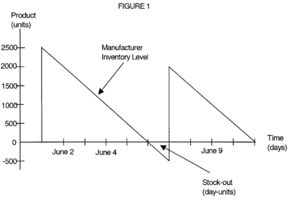
Perhaps the best starting point of a discussion about inventory stock-outs is a review of the classical inventory model represented by a saw-tooth curve. This model plots time on the horizontal axis and a firm's inventory level on the vertical axis, thereby measuring how the firm's inventory level changes over time. Figure I shows an example of such a system.
This firm's inventory system begins with zero inventory at the start of business on June 1. Immediately, a shipment of 2500 units is received, raising the inventory to 2500 units. From then on, customer demand depletes inventory at a constant rate of 500 units per day. At the start of June 6, inventory reaches zero, and the firm experiences an inventory
FIGURE 1 Product (units) 250G-- Manufacturer Inventory Level 2000-- 1500--100(7 -500- -0 |Time
June 2 June 4 June 9 (days)
-500-Stock-out
(day-units)
backorders.' Finally, at the start of June 7, a shipment of 2500 units is received, the
stock-out ends, and the inventory cycle repeats.
3.13 Quantifying Stock-outs - A Definition of Stock-out Magnitude
Between the start of June 6 and June 7, a stock-out situation exists. Because customer orders are continuous, the magnitude of the stock-out can be defined and measured in
terms of day-units as the integral of the customer order curve, evaluated for the duration
of the stock-out. In this case, the area under the curve between June 6 and June 7, or 250 day-units, quantifies the stock-out.
1 During a period when a firm has no inventory to meet customer demand, it may either accumulate this
demand in the form of backorders which will be filled as soon as inventory becomes available, or it may experience lost sales. This thesis will assume that firms accumulate backorders in all examples.
This day-unit measure is useful because it captures both the quantity and time dimensions of stock-outs. Only considering the quantity aspect of stock-outs would be misleading because a stock-out of 500 units that only lasts one day is certainly not as severe as a stock-out of the same quantity that lasts for ten days. Similarly, only considering the time aspect of stock-outs would not differentiate between a relatively minor shortage of ten units over three days and a relatively large shortage of one thousand units over the same three days.
3.2 What Causes Stock-outs?
Many causes for inventory stock-outs exist. Some possibilities include, but are not limited to: actual customer demand in excess of forecasted customer demand; suppliers shipping less than ordered quantities; and inventory lost to defects, spoilage, failure testing, pilferage, or uses other than the intended uses (Bernard, 1999). These various causes will be classified in Section 3.3. However, before attempting to categorize the causes, it is first helpful to gather information about the events and actors in a supply chain that drive stock-out occurrences.
3.21 Variance between Planned and Actual Inventory System Performance To determine the cause of an inventory stock-out, it is necessary to compare the actual performance of an inventory system to some ideal, or planned performance. The difference between the two will be referred to in this thesis as variance.
The actual performance of an inventory system usually occurs at an operational level that changes daily or hourly. In contrast, the planned performance of an inventory system usually occurs at a tactical level that changes weekly or monthly (Ballou, 1992). When a firm forecasts customer demand or places orders with its suppliers based on the suppliers' leadtimes several weeks in advance, it is planning on a tactical level; whereas, when the
same firm plans detailed delivery schedules based upon final customer orders or releases received a few days before shipment, it is executing on an operational level.
FIGURE 2 Product (units) June 2 June 4 Actual Planned Time (days) Variance (day-units)
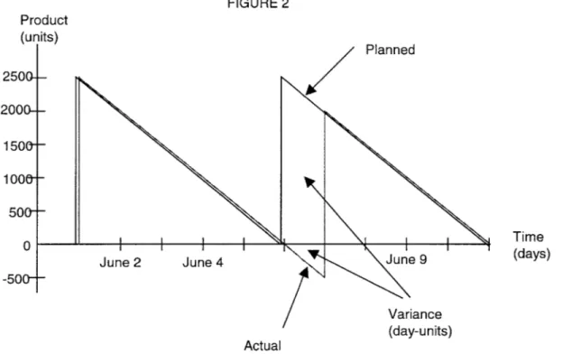
In order to compare the planned and actual performance of an inventory system, it is helpful to plot both curves on the same graph as two related saw-tooth curves (Tersine,
1988). In Figure 2, the same inventory stock-out illustrated previously in Figure 1 is graphed and labeled as the actual inventory performance curve. In addition to this curve,
1 1
the planned inventory performance curve shows the inventory level the firm expected to maintain. This curve shows that the 2500 units of inventory that are actually received on June 7 were in fact planned to be received on June 6. Because the inventory is actually
received one day later than planned, a stock-out occurs with a duration of one-day.
When the firm makes tactical plans, it normally does not plan to run short of inventory. Therefore, the planned performance level should show a positive, or at least a zero
inventory level. On the other hand, because the actual performance level is subject to random variation in customer demand and supplier delivery, it may show instances of inventory stock-outs in spite of the planning.
It is possible to measure the difference between the two curves using the same unit of measure used for stock-outs. In Figure 2, the variance between the actual and planned curves is 2500 day-units. Intuitively, this measurement makes sense because a delivery quantity of 2500 units is delayed by one day, and the product of 2500 units and one day is equal to 2500 units. However, the magnitude of the stock-out remains only 250 day-units, or the portion of the variance that lies below the zero-inventory axis.
With the context of the planned inventory performance, it is now possible to deduce that the cause of the inventory stock-out is the 2500-unit delivery that takes place on June 7 instead of June 6. However, it is still not certain why the delivery is later than planned. The late delivery might be the result of a delay in the supplier's production schedule, inclement weather affecting the transportation of the delivery, or even the firm itself
having sent its supplier the order for the June 6 delivery with an insufficient leadtime. Thus, this comparison of actual and planned inventory performance can only identify how certain events cause an inventory stock-out. Sections 3.23 and 3.24 will build a
framework for analyzing the causes behind such events.
3.22 Safety Stock Levels as an Influence upon Stock-outs
Before building this framework, however, it is important to address the issue of safety stock as one special factor that influences stock-outs. As mentioned in Section 3.3, firms do not typically plan to run short of inventory. Unlike the planned inventory performance curve shown in Figure 2, most firms recognize the random nature of supply and demand and plan to replenish their inventories well before they reach zero by reserving a certain amount of safety stock.
However, probabilistic inventory models show that as the service level of an inventory system approaches 100%, the expense of holding safety stock increases substantially. As this expense of holding safety stock approaches the expenses associated with an
inventory-stock-out, many firms plan to endure the stock-outs that are less expensive than the safety stock investments needed to prevent them. This trade-off between the costs of holding safety stock and the costs associated with stock-outs means that anytime a firm chooses a particular safety stock level, it automatically plans that a certain amount of stock-outs will statistically occur.
Thus, the cause of any stock-out that occurs within the amount of stock-outs statistically implied by a firm's safety stock level might be attributed to the firm's own inventory policy. While this is certainly true, this issue is separate from the one treated in this thesis. Comparing the actual number of inventory stock-outs to the number statistically predicted by the firm's inventory model might be useful in determining the robustness of the firm's model, but it does not directly help in determining which events in the model contribute the most to stock-outs.
3.23 A Supply Chain Model
Section 3.21 showed how a comparison of planned and actual inventory performance can identify a specific event, such as a late supplier delivery, to be the cause of a stock-out. However, this type of comparison does not explain which party associated with the event actually caused it. For example, in the case of the late supplier delivery, either the supplier or the manufacturer could have caused the delivery to be late. In order to determine which party was the cause, it is helpful to construct a supply chain model which lists the parties and how they interact. This section will describe the supply chain model which will be used in future examples throughout this thesis.
3.231 Description of the Model
Figure 3 shows a simple model that involves only three parties and only three types of parties: (1.) one supplier, (2.) one manufacturer, (3.) and one customer. The
raw material into only one finished product in a single-step manufacturing process, and delivers it to only one customer.
FIGURE 3. - A SUPPLY CHAIN MODEL
2. Purchase order (P.O.) 5. Customer order (C.O.)
3. Delivery (receipt) 6. Delivery (shipment)
MANUFACTURER
4. Production
CUSTOMER
1. Forecast
The model includes two types of transactions between the three parties involved: information exchanges and material exchanges. Information flows up the chain (from right to left, in Figure 3.) from the customer back to the supplier. In return, material flows down the chain (from left to right) from the supplier out to the customer. Of course, the financial exchanges that match the material exchanges are the third important type of transaction in a supply chain; however, these do not directly affect inventory performance and are therefore not included in the model.
Six events, or steps, take place to coordinate the flow of all information and material in the system. In Step 1, the customer transmits a forecast of future orders to the
manufacturer. Next, in Step 2, the manufacturer places orders with the supplier based on SUPPLIER
the customer's forecast. In Step 3, the supplier delivers the raw materials ordered in Step 2. Since this system has been constructed from the perspective of the manufacturer, this thesis refers to supplier deliveries made in Step 3 as "receipts". Once the manufacturer has received the raw materials, it then proceeds to the manufacturing process in Step 4. In Step 5., the customer sends a firm order to the manufacturer. Finally, in Step 6, the manufacturer delivers the final product to the customer. This thesis refers to this kind of delivery in Step 6 as a "shipment", again from the perspective of the manufacturer, in order to distinguish it from the deliveries known as receipts in Step 3.
In general, the steps of the model will follow a linear sequence, but in some cases, parallel sequences may occur. For example, Steps 1, 2, 3, 4, and 6 form one sequence of information and material flows that must occur in order. Simultaneously, Steps 1, 5, and 6 form another sequence that must also flow in order. Observing these two parallel sequences, it is clear that the occurrence of Step 5 is independent of Steps 2, 3, and 4. Although it is most likely to occur close in time to Steps 3 and 4, the only restriction is that it takes place after Step 1 and before Step 6. As the number of parties modeled grows, the number of parallel sequences will also necessarily grow.
3.232 Simplification of the Model
The choice of how simple the model should be depends on the level of detail required in the stock-out causes that the model is designed to illuminate. For example, when
considering the late delivery described in Section 3.21, the supply chain model in Figure 3 will be sufficient to determine whether the supplier's actions or the manufacturer's
actions caused the delay. However, if the actions of an intermediate transportation firm must be evaluated, or if the actions of the sales and purchasing functions of the
manufacturer must be evaluated, a more complicated supply chain model that includes these parties would be necessary.
3.233 Variations on the Model
The rather simple structure of the model in Figure 3 does not begin to illustrate the many possible variations that are found in actual inventory systems. While this model includes only one firm for each type of party, most inventory systems are networks where multiple parties participate at each level of the supply chain. For example, many firms source raw
materials from more than one supplier and provide the same finished product to more than one customer. Also, most manufacturing processes involve the combination of multiple raw materials together to make one finished product. Furthermore, many manufacturing processes take more than one step to complete.
In addition to variations in the number of parties, products and processes modeled, variations in the configuration of the model are also possible. For example, this model
assumes that customers submit a forecast to manufacturers of future orders; whereas in practice, many manufacturers must generate forecasts without any direct customer input. Therefore, the simple example in this thesis will necessarily be structurally different from most systems found in practice. However, the principles used to develop this model of a hypothetical supply chain should be applicable to the modeling of any real supply chain.
3.24 A Supply Chain Transaction Log
Having described the various parties of the supply chain model in Section 3.23, it is next necessary to observe the transactions among them that determine the cause of an event leading to a stock-out. For instance, by knowing when a manufacturer sent its supplier a purchase order, when the supplier delivered its product to the manufacturer, and how long the supplier's leadtime was, it is possible to determine which party's actions caused the supplier's late delivery. This section will develop a transaction log with the pertinent data needed to determine the causes of inventory stock-outs.
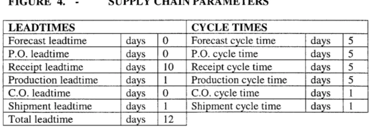
3.241 Supply Chain Parameters
Before considering actual transactions, it is necessary to establish the parameters that govern the transactions. Figure 4 shows in tabular format the two types of parameters that will be used in this thesis: leadtimes and cycle times.
FIGURE 4. - SUPPLY CHAIN PARAMETERS
LEADTIMES CYCLE TIMES
Forecast leadtime days 0 Forecast cycle time days 5
P.O. leadtime days 0 P.O. cycle time days 5
Receipt leadtime days 10 Receipt cycle time days 5
Production leadtime days 1 Production cycle time days 5
C.O. leadtime days 0 C.O. cycle time days 1
Shipment leadtime days 1 Shipment cycle time days 1
In this thesis, the leadtime is defined as the amount of time required to complete a step, once the previous step has been completed. Thus, once raw materials have been received from the supplier in Step 3, it is possible for the manufacturer to transform the raw materials into the finished product in one day. This definition assumes a few things. First, it assumes that production can be both scheduled and completed by the
manufacturer in one day. If the manufacturer had limited production capacity and many different products to produce, then any order received might be queued into a list of orders waiting for line time. In such a case, the majority of the leadtime might be waiting time as opposed to actual production time. Second, the definition assumes that the order is of sufficient quantity to warrant an entire production run. If the order were relatively small in quantity, then it might again be queued into a list of orders waiting for other similar orders to reach a certain minimum production quantity. Finally, the leadtime assumes enough time to produce the entire run.
Next, the cycle time of a step in the supply chain will indicate the frequency with which that step usually occurs. This will be defined as the amount of time it takes for the next step to consume the average batch size of that step. For example, the manufacturer's production process (Step 4) is shown to take place every five days, shown by the 5-day cycle time in Figure 4.
3.242 Supply Chain Transaction Data Elements
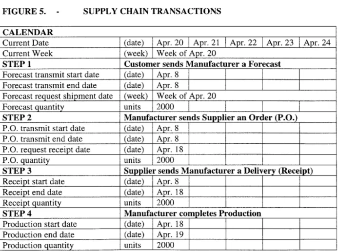
Figure 5 introduces in tabular format some data about sample transactions that occur within the supply chain model developed in Section 3.3. In addition to providing the
sample data, the table also demonstrates the data elements required to describe the transactions.
The first rows of the table display a calendar around which the data is organized. The calendar at the top of the chart does not establish columns to indicate when each step occurs. Instead, the columns indicate with which customer order due date the events are related. For example, the first column titled April 20 contains a purchase order sent on April 8 for material to be received on April 18. This means that the material to be transferred on this purchase order has been prepared for the purpose of filling a customer order due on April 20.
FIGURE 5. - SUPPLY CHAIN TRANSACTIONS
CALENDAR
Current Date (date) Apr. 20 Apr. 21 Apr. 22 Apr. 23 Apr. 24 Current Week (week) Week of Apr. 20
STEP 1 Customer sends Manufacturer a Forecast
Forecast transmit start date (date) Apr. 8 Forecast transmit end date (date) Apr. 8
Forecast request shipment date (week) Week of Apr. 20 Forecast quantity units 2000
STEP 2 Manufacturer sends Supplier an Order (P.O.)
P.O. transmit start date (date) Apr. 8 P.O. transmit end date (date) Apr. 8 P.O. request receipt date (date) Apr. 18
P.O. quantity units 2000
STEP 3 Supplier sends Manufacturer a Delivery (Receipt)
Receipt start date (date) Apr. 8 Receipt end date (date) Apr. 18
Receipt quantity units 2000
STEP 4 Manufacturer completes Production
Production start date (date) Apr. 18 Production end date (date) Apr. 19 Production quantity units 2000
STEP 5 Customer sends Manufacturer and Order (C.O.) C.O. transmit start date (date) Apr. 19 Apr. 20 Apr. 21 Apr. 22 Apr. 23 C.O. transmit end date (date) Apr. 19 Apr. 20 Apr. 21 Apr. 22 Apr. 23 C.O. request shipment date (date) Apr. 20 Apr. 21 Apr. 22 Apr. 23 Apr. 24
C.O. quantity units 400 400 400 400 400
STEP 6 Manufacturer sends Customer a Delivery (Shipment)
Shipment start date (date) Apr. 19 Apr. 20 Apr. 21 Apr. 22 Apr. 23 Shipment end date (date) Apr. 20 Apr. 21 Apr. 22 Apr. 23 Apr. 24
Shipment quantity units 400 400 400 400 400
ANALYSIS C.O. vs. Shipment Balance
C.O vs. Shipment Balance units 0
|0
0 0 0There are four data elements needed to completely describe information transfers in this model: (1.) the start time of the transfer, (2.) the end time of the transfer, (3.) the time period that is the subject of the transfer and (4.) the quantity of material that is the subject of the transfer. For example, in Step 1., (1.) the customer sends the manufacturer a forecast on April 8, (2.) the manufacturer receives the forecast on April 8, (3.) the forecast is for the week of April 20, and (4.) the forecast quantity is 2000 units.
Given that much information exchanged between businesses today takes place via
telephone, fax or e-mail, the distinction between start and end times of these transfers will not always be important. For example, in Step 1, the time that the customer sends the forecast and the time that the manufacturer receives the forecast are the same day, April 8. Accordingly, the forecast leadtime in Figure 4 is a zero leadtime, indicating that the time to transmit the forecast is practically instantaneous. However, if the manufacturer were to use a queuing process to review forecast information, or if forecasts are sent via surface mail, then the start and end times of information transfers could become important.
There are only three data elements required to describe material transfers in this model: (1.) the start time of the transfer, (2.) the end time of the transfer, and (3.) the quantity of the transfer. The period that is the subject of the transfer is assumed to be the same period in which the transfer takes place. For example, in Step 6., (1.) the manufacturer sends the customer a shipment on April 19, (2.) the customer receives the shipment on April 20, and (3.) the shipment is for 400 units.
It is important to note that not all of the data elements listed in this section are necessary for a meaningful stock-out cause analysis. For example, a manufacturer attempting to conduct a stock-out cause analysis may only know the dates when it receives its supplier deliveries, not the dates when the supplier actual begins the process of supplying the material. That is, the manufacturer knows the Step 3 end date, but not the Step 3 start date. In this case, it is still possible to conduct an analysis by comparing the known Step
3 end date with Step 2 data. However, the manufacturer will only be able to determine whether a supplier delivery was late, and not whether it was late because the supplier started its process too late or because its process took too long. Whether the supplier started late or took to long may or may not be an important issue, depending on the goals of the manufacturer conducting the analysis. Thus, depending on the actual visibility of the data in the supply chain, the selection of data elements described here can be modified to suit the purposes of the user.
3.243 Graphical Representation of Transactions
Figure 6 graphically represents the transactional data using the same representation of inventory level over time used by the classical saw-tooth curve. As the graph shows, there is no variation between actual and planned inventory performance for the sample data given in Section 3.242, and therefore, there is no occurrence of a stock-out. However, below are a few issues that arise when applying this representation to transactional data.
Unlike the theoretical curves shown in Figures 1 and 2, however, the model shown in Figure 6 is discrete, not continuous. This reflects the actual nature of most inventory systems, where movements in inventory are made in discrete quantities, as well as the actual nature of the data, which is recorded in discrete transactions. Because the inventory level of the system described by this model changes from day to day with additions through production and subtractions through shipments, the discrete movements of the inventory level will be graphed in terms of days.
Also, because of the one-day leadtime required to ship a customer order, Figure 6 necessarily shows the inventory position of the manufacturer one day prior to the
customer order due date used in Figure 5. This is because the transaction data in Figure 5
is organized around the customer order due date and customer forecast, and the inventory performance data in Figure 6 is organized around how manufacturer's inventory
Product FIGURE 6 (units) 2000- 1800- 1600- 1400-Forecast 1200 - 1000- 800- 600-400- Actual 200-0- 0 ITime (date in April) -200_ 19 20 21 22 23 24 -400- -600- -800-
-1000-Further, not all steps of the transaction log show up directly in the graphical
representation. In this model, Step 1. of the system, or the forecast, becomes the planned
inventory performance level shown in Figure 6. Next, Steps 4 and 6 describe the actual
inventory performance of the model. Lastly, Steps 2, 3 and 5 describe intermediate steps
in the model that contribute to the actual inventory performance of the model.
Finally, in the sample transaction log in Figure 5, the forecast is given in terms of units
between the two units of measure, this model will assume that planned shipments will occur uniformly throughout the forecast period. In a more complicated model, the units of measure for each exchange of information or material and any assumptions necessary to convert the units of measure would have to be included in the parameters of the model.
3.244 Narration of Sample Transactions
Given these leadtimes and cycle times, Figure 5 shows us the flow of information and material required for the manufacturer to supply product to the customer during the week of April 20th.
STEP 1. First, on April 8th, the customer sends the manufacturer a forecast of orders for the week of April 20th. This forecast is sent within the total 12-day leadtime needed by the manufacturer for on-time delivery.2 The transmission of the forecast itself is considered to occur instantaneously, with no delays, as if it were communicated via telephone, fax, or e-mail. The forecast quantity is for 2000 units.
STEP 2. Immediately after receiving the forecast, the manufacturer then transmits an order to the supplier for 2000 units of raw material to be delivered on April 18th. This order takes place within the 10-day receipt leadtime. Again, the order is considered to transmit instantaneously.
STEP 3. As promised, on April 18th, the supplier delivers 2000 units to the manufacturer.
STEP 4. Once the raw material has been received on April 18th, it then takes one day for it to be transformed into finished product, completing 2000 units by April 19th.
STEP 5. Also on April 19th, the customer sends the manufacturer a firm order for 400 units of finished product to be delivered on April 20th. Again, the order transmission takes place instantaneously. Also, over the following four days, four more orders for deliveries within the week of April 20th are also sent. The total quantity of the sum of five orders sent equals the original forecast quantity of 2000 units exactly.
STEP 6. After receiving the first order on April 19th, the manufacturer then has the full one day needed to ship the product to the customer on time, on the requested delivery
date of April 20th. The next four orders are shipped out on time as well.
3.3 What kinds of stock-out causes exist?
Having discussed the events and parties involved in a supply chain which cause inventory stock-outs, it is now possible to classify the causes.
3.31 Two Dimensions of Stock-outs - Quantity and Time
In this thesis, a stock-out has been defined as a situation when customer orders exceed the manufacturer's inventory of finished product. Such a situation appears in the transaction
log as either a late delivery to the customer, a "short"3 delivery to the customer, or a late
and "short" delivery to the customer. That is, any situation in which the manufacturer cannot perform Step 6 in accordance with the customer's request in Step 5.
The customer orders in the transaction log have only two parts: (1.) a demanded quantity of product, and (2.) a delivery due date. These two aspects of customer orders represent the two dimensions along which a stock-out can occur. A short delivery represents a
shipment whose quantity does not meet the order, and a late delivery represents a
shipment whose delivery date is past due. These two dimensions are also reflected in the day-units measure used to quantify stock-outs. Units measure quantity, and days measure lateness of shipments.
Of course, customer orders typically have more than these two simple elements. Most firms include many requirements related to the quality of product purchased on their orders, including a detailed product specification, packaging requirements, requested delivery mode, and other factors. In actuality, these quality-related aspects of orders relate to stock-outs in terms of the quantity of finished product they affect. Any failure of the manufacturer to meet quality-related aspects of a customer order effectively reduces the quantity of usable, delivered product by the customer. For example, suppose the customer orders 100 units of a specific product specification to be delivered on June 1. If the manufacturer delivers 100 units on June 1, but only 90 units meet the product
specification, the customer has only 90 units available to move to the next step in
3 In this thesis, the informal yet convenient term,"short", will be used to describe both supplier deliveries
and manufacturer shipments whose quantity is less than the corresponding purchase order or customer order.
production. The end result from the perspective of the next step in the supply chain is the same as if only 90 units, or an insufficient quantity, were delivered.
3.32 Classification Codes
Having identified quantity and time as two dimensions of outs, the causes of stock-outs also fall into these same two categories: those that are quantity-based and those that are time-based. Quantity-based causes occur because of a loss of product quantity in the system, and time-based causes happen because of a delay of product in the system.
Careful consideration of the time-based causes yields two different types within this category which may be referred to as "postponed" and "retarded". Postponed time-based causes are ones that involve one of the steps starting too late relative to the order due date and the given leadtimes of all steps yet uncompleted. Retarded time-based causes are ones that involve one of the steps taking too long from start to finish relative to the given leadtime of the step.
In addition to classifying causes by the ways in which they affect the timing and quantity of shipments to customers, we can also classify them by the step in the supply chain which generates them. For example, a quantity-based cause might originate in the purchase order of step 2 or in the production of step 4.
In order to label these various classifications of stock-out causes, we can use a simple coding system. To distinguish between the first classification described, we can use the letter "Q" for quantity-based causes, the letter "P" for postponed time-based causes, and the letter "R" for retarded time-based causes. Next, we can use the numbers 1 through 5
6 is the step where outs are identified, it cannot be included in the causes of stock-outs.) Combining these letters and numbers, we now have 15 possible reasons for a stock-out in our system. For example, 2Q would refer to a quantity-based reason that occurs at step 2. That is, the situation where the quantity of a purchase order issued to the supplier was insufficient with respect to the original forecast.
3.4 How do multiple stock-out causes interact?
In a complex inventory system with multiple actors and numerous steps in the supply chain, any given inventory stock-out occurrence is likely to be the result of more than one cause. Even in a relatively simple system, multiple causes are still likely to be common; therefore, it is important to consider how multiple causes interact. Whereas Sections 3.1 through 3.3 only considered stock-outs with a single cause rooted in a single event, Section 3.4 will discuss how to treat stock-outs with multiple causes resulting from multiple events.
3.41 Methodology for Understanding Multiple Cause Interaction
Naturally, the same set of events and parties which lead to the single causes of stock-outs also lead to the multiple causes. Further, the same method of classification applies to both situations. What is different in the case of multiple causes is that the magnitude of the stock-out must be shared by more than one cause. The classical saw-tooth inventory model is useful to propose how stock-out magnitude should be divided among multiple stock-out causes. A discrete, transaction-based model could also be used, but the continuous model makes the graphical representation of the division easier to illustrate.
In order to determine the magnitude of the stock-out contributed by each individual cause, it is first necessary to imagine individual scenarios for each cause occurring in isolation. That is, instead of simply comparing the system's planned and actual inventory
performances, the planned performance must be compared to a range of scenarios in which all of the events in the system occur according to plan with the exception of one event that contributes to the stock-out.
When the stock-out magnitudes for each individual scenario are totaled, the resulting magnitude is not necessarily equal to the actual stock-out magnitude. The interaction of multiple causes of a stock-out may cause the individual magnitudes to overlap with each other and produce a stock-out with smaller magnitude than the sum of the individual parts. Alternatively, the interaction of the multiple causes may compound the effects of the individual magnitudes to generate a stock-out with a larger magnitude than the sum of the individual parts.
3.42 Overlapping Multiple Stock-out Causes
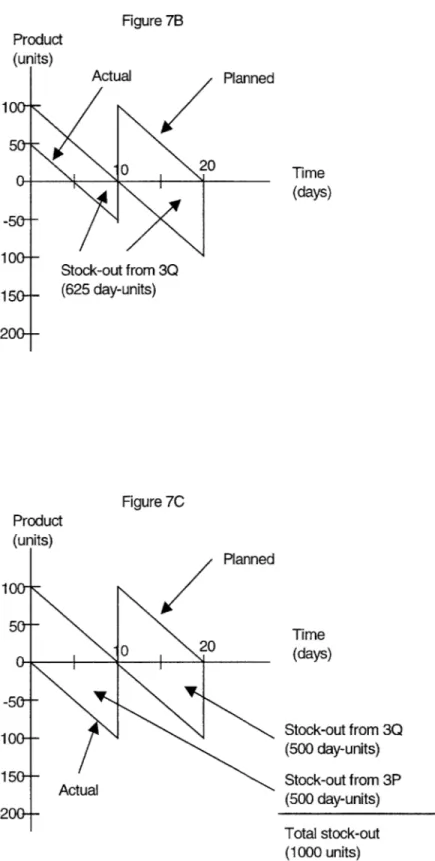
An example where supplier deliveries are both late and "short", or a situation combining both time- and quantity-based stock-out causes, is one such situation where causes may overlap to diminish the magnitude of the stock-out. Figures 7A through 7C show an inventory system with a planned supplier delivery of 100 units every ten days and a planned customer demand of 10 units per day. Over a twenty-day period, two supplier deliveries are made, one on day zero, and one on day ten. Figure 7A illustrates the
outcome of the first supplier delivery arriving ten days late. This cause could be
classified as either cause 3P or cause 3R, but this example will assume cause 3P. Figure 7B shows the result of both supplier deliveries arriving 50 units short, or cause 3Q. Finally, Figure 7C demonstrates the outcome of both causes acting together.
Figure 7A Product (units) Planned 100--0 20 Time 0 | | | 1(days) -1 -1 Stock-out from 3P (500 day-units) Actual
Figure 7B Product Planned Time (days) Stock-out from 3Q (625 day-units) Figure 7C Product (units) Planned Time (days) Stock-out from 3Q (500 day-units) Stock-out from 3P (500 day-units) Total stock-out (1000 units) Actual 1 1001 50 0 0 20 -50f -100--150-f -20(4 Actual ' , V-1
Cause 3P alone generates a stock-out of 500 day-units, and cause 3Q alone generates a stock-out of 625 units. Taken together, they result in a stock-out of only 1000 day-units.
As Figure 7C shows, we can partition these 1000 day-units into those directly attributed to cause 3P and those directly attributed to cause 3Q. To understand why, it is helpful to imagine how the manufacturer's inventory is affected. The first 500 day-units are
attributed to cause 3P because of the late delivery. Between day zero and day ten, the late delivery accumulates the 500 day-units regardless of the quantity of the order. On day ten, both orders arrive, and at this point, none of the orders are late. Between day ten and day twenty, the 500 day-units accumulated can only be attributed to the fact that both deliveries were short.
The difference between the isolated cases and the aggregate case is the fact that 125 day-units would have accumulated between day five and day ten if the orders were all on time, yet delivered short. In the aggregate case where the first order is ten days late, these 125 day-units cannot be accumulated because they are masked by the late order.
3.42 Accumulating and Compounding Multiple Stock-out Causes
Next, suppose a situation where the multiple causes together generate a stock-out whose magnitude is greater than the sum of the individual magnitudes. A situation where customer demand is greater than forecasted and supplier deliveries less than ordered, or a situation combining both two quantity-based stock-out causes, can illustrate one such example. For instance, Figures 7D through 7F show the same inventory system described earlier under different stock-out conditions. Figure 7D shows exactly the same short supplier deliveries (cause 3Q) illustrated in Figure 7B. Figure 7E shows the system faced
with a doubling of customer demand (cause 5Q). Finally, Figure 7F combines the causes of Figures 7D and 7E together.
Cause 3Q alone generates a stock-out of 625 day-units, and cause 5Q alone generates a stock-out of 1250 units. Taken together, they result in a stock-out of 2562.5 day-units. Figure 7D Product (units) Actual Planned 020 Time (days) -5 -- -100--Stock-out from 3Q -150 (625 day-units)
-200--As Figure 7F shows, we can partition these 2562.5 day-units into those directly attributed to cause 3Q, those directly attributed to cause 5Q, and those attributed to the combination of causes 3Q and 5Q. Unlike the combination of time-based and quantity-based causes within the same time period shown earlier, the combination of quantity-based causes results in an accumulation and compounding of stock-out magnitude. That is, quantity-based causes do not overlap, they exaggerate their individual effects. Because of this
behavior, it is true that 625 day-units of the stock-out shown in Figure 7F are attributable to cause 3Q, 1250 day-units to cause 5Q, and the remaining 687.5 day-units to the combination of 3Q and 5Q. Figure 7E Product (units) Planned 100- 50--00 0 Time (days) -50 -Stock-out from 5Q -100-- (1250 day-units) -150-- _Actual
-200--One thing that cannot be determined is which day-unit of a stock-out on any given day is assigned to a particular cause. The graphical representation of the partitioning shown in Figure 7F is arbitrary and illustrated with the aim of being easy to read. In actuality, there is no preference to either cause 3Q or 5Q as to which should claim the first day-units of a
stock-out. For example, on day fifteen, the graph shows cause 3Q as the cause of the first 50 units of the stock-out, the combination of causes 3Q and 5Q as the cause of the nest 50 units, and cause 5Q as the cause of the remaining 100 units. Even though cause 3Q happens earlier in the supply chain sequence than cause 5Q, there is no logical basis for
causes occur independently, and therefore have no claim on any particular division of the stock-out. Figure 7F Product (units) Time (days) A - Stock-out from 3Q (625 day-units) B - Stock-out from 5Q (1250 day-units) C - Stock-out from 3Q/5Q (687.5 day-units) Total stock-out (2562.5 day-units)
3.5 How to Identify Stock-outs?
The causes of stock-outs may be determined by using the sort of transaction data
described previously. This section will introduce some sample data in Section 3.51, identify quantity-based stock-out causes in Section 3.52, identify postponed time-based stock-out causes in Section 3.53, and finally identify retarded time-based stock-out causes in Section 3.54.
3.51 Sample data
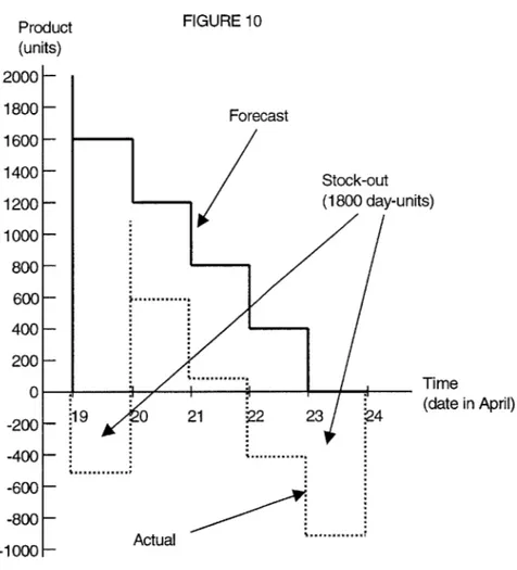
Figure 8 repeats the same inventory system parameters given in Figure 4, and Figure 9 uses the same tabular format developed in Section 3.24 to show transaction data that illustrates an inventory stock-out. Figure 10 graphically represents the actual and planned inventory performance of the system.
FIGURE 8. - SUPPLY CHAIN PARAMETERS
LEADTIMES CYCLE TIMES
Forecast leadtime days 0 Forecast cycle time days 5 P.O. leadtime days 0 P.O. cycle time days 5 Receipt leadtime days 10 Receipt cycle time days 5 Production leadtime days 1 Production cycle time days 5
C.O. leadtime days 0 C.O. cycle time days 1
Shipment leadtime days 1 Shipment cycle time days 1 Total leadtime days 12
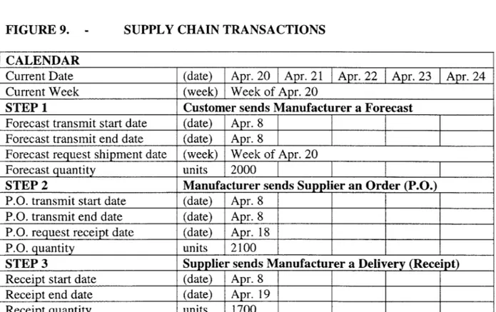
FIGURE 9. - SUPPLY CHAIN TRANSACTIONS
CALENDAR
Current Date (date) Apr. 20 Apr. 21 1 Apr. 22 Apr. 23 Apr. 24 Current Week (week) Week of Apr. 20
STEP 1 Customer sends Manufacturer a Forecast
Forecast transmit start date (date) Apr. 8 Forecast transmit end date (date) Apr. 8
Forecast request shipment date (week) Week of Apr. 20 Forecast quantity units 2000
STEP 2 Manufacturer sends Supplier an Order (P.O.)
P.O. transmit start date (date) Apr. 8 P.O. transmit end date (date) Apr. 8 P.O. request receipt date (date) Apr. 18
P.O. quantity units 2100
STEP 3 Supplier sends Manufacturer a Delivery (Receipt)
Receipt start date (date) Apr. 8 Receipt end date (date) Apr. 19 Receipt quantity units 1700
STEP 4 Manufacturer completes Production Production start date (date) Apr. 19
Production end date (date) Apr. 20 Production quantity units 1600
STEP 5 Customer sends Manufacturer and Order (C.O.)
C.O. transmit start date (date) Apr. 19 Apr. 20 Apr. 21 Apr. 22 Apr. 23 C.O. transmit end date (date) Apr. 19 Apr. 20 Apr. 21 Apr. 22 Apr. 23 C.O. request shipment date (date) Apr. 20 Apr. 21 Apr. 22 Apr. 23 Apr. 24
C.O. quantity units 500 500 500 500 500
STEP 6 Manufacturer sends Customer a Delivery (Shipment)
Shipment start date (date) Apr. 20 Apr. 20 Apr. 21 Apr. 22 Apr. 23 Shipment end date (date) Apr. 21 Apr. 21 Apr. 22 Apr. 23 Apr. 24
Shipment quantity units 500 500 500 100 0
ANALYSIS C.O. vs. Shipment Balance
C.O vs. Shipment Balance units (500) 0 0 (400) (900)
The following is a narrative description of the data in Figures 9 and 10.
STEP 1. The initial conditions for both Figures 5 and 9 are identical, starting with a customer forecast of 2000 units for the week of April 20th.
STEP 2. The manufacturer inflates the purchase order quantity by 100 units above the customer's forecast. This might be due to market speculation, knowledge of the customer's previous forecast performance, knowledge of the supplier's previous delivery performance, or a simple typographical error.
STEP 3. The supplier delivers material on the purchase order one day late on April 19 and is 400 units short of the quantity ordered, 1700 units vs. 2100 units.
STEP 4. For some unpredicted reason, the manufacturer loses 100 units of material in the production process and only generates 1600 units of finished product.
STEP 5. On top of this, the customer issues orders for the week of April 20th totaling 2500 units, or 500 units above that originally forecasted.
FIGURE 10 Forecast Stock-out (1800 day-units) "I/' Product (units) 2000- 1800- 1600- 1400- 1200- 1000- 800- 600- 400- 200-0-. -200_ -400- -600--800 -1000 Time (date in April)
STEP 6. In response to the first order of 500 units due April 20, the manufacturer has no inventory due to the late supplier receipt which has in turn delayed the production
and shipment by one day. On April 21, the manufacturer makes up for the April 20 backorder and ships 1000 units to cover all outstanding orders. Next, on April 22, the
20 21 22 23 24
manufacturer ships another 500 units, leaving only 100 units left in inventory. Thus, on April 23, the manufacture can only ship 100 units, accumulating a 400-unit backorder. Finally, on April 24, the backorder increases by another 500 units to a total of 900 units.
3.52 Test to Identify Quantity-based Stock-out Causes
Quantity-based stock-out causes can be identified through transactional data by subtracting the quantity of a given supply chain step from the quantity of the previous sequential supply chain step. The result is the variance associated with the quantity-based stock-out cause of the supply chain step. A positive test result for a valid stock-out cause is a positive value.
For example, to identify cause 3Q from the transactional data in Figure 9, it is necessary to subtract the quantity of Step 3, or 1700 units, from the quantity of Step 2, or 2100 units. Because the result is 400 units, cause 3Q is one valid cause of the stock-outs described in Figure 9.
Incidentally, the step in the model which is identified with the planned inventory performance cannot be a quantity-based stock-out cause. Obviously, this is because
whatever baseline is established as the ideal performance level cannot contribute to a stock-out. Also, the units of measure of the cycle times of the steps compared in the calculation of this test must match; otherwise a conversion becomes necessary. For example, the customer orders issued in units per day cannot be directly compared to customer forecasts issued in units per week without a conversion. Likewise, shipments
with a cycle time of one day cannot be directly compared to production with a cycle time of five days.
Figure 11 below shows the results of the test for quantity-based stock-outs for each step of the transactional data. This table shows that causes 3Q, 4Q and 5Q are valid stock-out causes.
FIGURE 11. - ANALYSIS OF QUANTITY-BASED STOCK-OUTS
Calendar date (date) 20 21 22 23 24
Cause 1Q Variance units n/a
Cause 2Q Variance units -100
Cause 3Q Variance units 400
Cause 4Q Variance units 100
Cause 5Q Variance units 100 100 100 100 100
Cumulative Variance units 500 600 700 800 900
C.O. vs. Shipment Balance units (500) 0 0 (400) (900)
3.53 Test to Identify Postponed Time-based Stock-out Causes
The test to identify postponed time-based stock-out causes begins with the date of the start of the transfer of the supply chain step involved. The date of the start of the transfer is compared to the corresponding customer order due date and relevant leadtimes. The essence of the test is to determine whether the step began with enough leadtime to complete the customer order.
For example, to identify cause 2P, the first step is to note that the date of the start of the purchase order transmission is April 8. The next step is to note that the customer order
corresponding to the purchase order is due on April 20. The difference between the two dates is 12 days; and the total leadtime to send a purchase order, and then receive, process and ship material is also 12 days. Because the purchase order was issued with enough time to ship the corresponding customer order, the test result is negative, and cause 2P is not a valid stock-out cause. Also, the difference between the total leadtime and the total process time allotted equals the variance associated with cause 2P, which in this case is zero.
In another example, to identify cause 4P, the first step is to note that the date of the start of production is April 19. The next step is to note that the customer order corresponding to the receipt is due April 20. The difference between the two dates is only one day; and the combined leadtime to produce and ship the material to the customer is two days. Because the receipt was not received with enough time to make the customer shipment on time, the test result is positive, and cause 4P is a valid stock-out cause. Also, the
difference between the two-day total leadtime and the one-day allotted time to complete the process is the variance associated with cause 4P, which in this case is one day.
Once one postponed time-based cause has been identified as a valid cause, the subsequent causes postponed time-based causes in the inventory system will also likely test positive, unless some event makes up for the time lost earlier in the sequence. Such related causes will often become multiple causes whose magnitude overlap, as discussed in Section 3.42.
Figure 12 below shows the results of the test for postponed time-based stock-outs for each step of the transactional data. This table shows that cause 4P is a valid stock-out cause.
FIGURE 12. - ANALYSIS OF POSTPONED TIME-BASED STOCK-OUTS
Calendar date (date) 20 21 22 23 24
Cause IP Variance days 0
Cause 2P Variance days 0
Cause 3P Variance days 0
Cause 4P Variance days 1
Cause 5P Variance days 0 0 0 0 0
3.54 Test to Identify Retarded Time-based Stock-out Causes
The test to identify retarded time-based stock-out causes compares the start and end dates of the transfer of the supply chain step involved. A positive test will yield a positive number when the relevant leadtime subtracted from the difference between the dates. This positive number is also the variance associated with the stock-out cause.
For example, to identify cause 3R, the first step is to calculate the difference between the start date of the receipt, April 8, and the end date of the receipt, April 19. The next step is to subtract the receipt leadtime of ten days from the difference of eleven days. The positive result of one day confirms that cause 3R is a valid stock-out cause with a variance of one day.
Figure 13 below shows the results of the test for retarded time-based stock-outs for each step of the transactional data. This table shows that cause 3R is a valid stock-out cause.