A Practical Approach to Model Predictive Control (MPC)for Solar Communities

(1)

UNIVERSITÉ DE MONTRÉAL

A PRACTICAL APPROACH TO MODEL PREDICTIVE CONTROL (MPC) FOR SOLAR COMMUNITIES

HUMBERTO QUINTANA

DÉPARTEMENT DE GÉNIE MÉCANIQUE ÉCOLE POLYTECHNIQUE DE MONTRÉAL

MÉMOIRE PRÉSENTÉ EN VUE DE L’OBTENTION DU DIPLÔME DE MAÎTRISE ÈS SCIENCES APPLIQUÉES

(GÉNIE MÉCANIQUE) JUIN 2013

(2)

UNIVERSITÉ DE MONTRÉAL

ÉCOLE POLYTECHNIQUE DE MONTRÉAL

Ce mémoire intitulé:

A PRACTICAL APPROACH TO MODEL PREDICTIVE CONTROL (MPC) FOR SOLAR COMMUNITIES

présenté par : QUINTANA Humberto

en vue de l’obtention du diplôme de : Maîtrise ès sciences appliquées a été dûment accepté par le jury d’examen constitué de :

M. BERNIER Michel, Ph.D, président

M. KUMMERT Michaël, Ph.D., membre et directeur de recherche M. SIBBITT Bruce, M.A.Sc., membre

(3)

(4)

ACKNOWLEDGEMENTS

It is curious that this page is the first one with prose when in the actual chronological order it is the last one. This is the personal touch that takes the mind away from the technical facts and allows remembering the path that has been followed and the people who were there for guiding, sharing, cheering or just observing. Please grant me the licence to be a bit informal on this page. First of all, a Big Thank You to my supervisor Michaël Kummert for the opportunity to work with him, his knowledge and positive attitude are inspiring (and his feedback very much needed). Same Big gratitude goes for Professor Michel Bernier; it has been an honor to be part of his group on Mécanique de Bâtiments (MecBat) at Polytechnique-Montréal. I also want to thank to Professor Alberto Teyssedou, Professor Oumarou Savadogo and Jean-François Desgroseillers, also from Polytechnique, for their advice and teachings.

Thanks to the SNEBRN research network for the funding for this research, and to John Kokko (Enermodal) and Bill Wong (SAIC-Canada) for making available all the needed documentation. At Natural Resources Canada, my appreciation goes to Doug McClenahan and Bruce Sibbitt for the interest on the development of this work; without the data, documents and feedback they provided, this research would have been impossible to carry out. I’m also grateful to Angela, David, Matt, Tim and Jeff from TESS for looking after me during my internship at their headquarters.

A special recognition to my hard-working colleagues in the MecBat team for their openness, cooperation and professionalism: Ali, Antoine, Aurélie, Benoit, Chiara, Katherine, Marilyne, Massimo, Mathieu(s), Mathilde, Roman, Parham, Yannick, and Vivien. Thanks to my brother, the family artist, for his help with certain figures. Special hugs travel the distance to reach my mother, my sisters, and my cousins, aunts and uncles; your love is very important in my life. Anna, Denise, Emmanuelle, Lidia, Maria Elena, Milena, Mónica, Verónica, Daniel, Edwin, Enrique, Harold, Juan Carlos, Ricardo, Sebastian and Thibaut; your support was also part of me achieving this goal.

Finally, a thankful smile to all those persons that may be never read this document but that directly or indirectly influenced my decisions, my thoughts and my motivation. In the same way, I hope this work will eventually have a positive influence in society.

(5)

RÉSUMÉ

Les réseaux de chaleur solaire (SDH pour Solar District Heating) font partie des solutions pour réduire la consommation d'énergie et les émissions de Gaz à Effet de Serre (GES) dues aux besoins de chauffage. Ce type d'installation permet de profiter des effets d’économie d’échelle et des avantages d'avoir un système centralisé qui facilite l’intégration de l'énergie solaire pour réduire la dépendance aux carburants fossiles. Un système SDH est un concept éprouvé qui peut être complémenté avec l'ajout de stockage à long terme de l'énergie thermique pour compenser le décalage dans le temps entre l'offre d'énergie solaire et la demande de la charge de chauffage. Ces systèmes sont surtout déployés en Europe; au Canada, la seule installation de SDH est la communauté solaire Drake Landing (DLSC pour Drake Landing Solar Community). Ce projet, qui comprend du stockage saisonnier (BTES pour Borehole Thermal Energy Storage), a été un grand succès, il a atteint 95% de fraction solaire à la cinquième année d'opération.

Un système SDH ne peut être complet sans un système de commande qui coordonne le fonctionnement et l'interaction des composants de l’installation. Le contrôle est basé sur un ensemble de règles qui prennent en considération l’état interne du système et les conditions extérieures pour garantir le confort des occupants avec un minimum de consommation de combustibles fossiles. Ce projet de recherche se concentre principalement sur la conception et l'évaluation des nouveaux mécanismes de commande visant à l'augmentation de l'efficacité énergétique globale des systèmes SDH. L'étude de cas est le projet DLSC, et les stratégies de commande proposées sont basées sur l'application pratique des concepts de la Commande Prédictive basée sur des Modèles (MPC pour Model Predictive Control).

Un modèle calibré de DLSC qui inclut les stratégies de commande a été développé dans TRNSYS, en s'appuyant sur le modèle utilisé pour les études de conception. Le modèle a été amélioré et de nouveaux composants ont été créés. Le processus de calibration a montré un très bon accord pour les indices annuels de performance énergétique (2% pour la consommation de gaz et pour la partie solaire de l’énergie thermique livrée au réseau de chaleur et, 5% pour la consommation d'électricité).

Les stratégies de commande proposées ont été conçues pour modifier quatre aspects du système du commande actuel: les paramètres qui définissent l'interaction entre le stockage de court terme

(6)

(STTS pour Short-Term Thermal Storage) et le BTES ont été optimisés pour faire en sorte que le STTS maintient un niveau plus élevé de charge lorsque le système est en mode hiver; une deuxième stratégie de contrôle oblige la décharge du BTES lorsque les conditions météorologiques prévues indiquent une forte charge de chauffage et/ou un rayonnement solaire réduit; les deux dernières stratégies ciblent la consommation d'électricité dans la boucle solaire et la boucle BTES en modulant la vitesse des pompes. Les résultats montrent que l'efficacité énergétique peut être améliorée d'environ 5% lorsque ces stratégies de commande sont utilisées avec des prévisions météorologiques parfaites.

(7)

ABSTRACT

Solar district heating (SDH) systems are part of the solution to reduce energy consumption and GHG emissions required for space heating. This kind of installation takes advantage of the convenience of a centralized system and of solar energy to reduce dependency on fossil-fuels. An SDH system is a proven concept that can be enhanced with the addition of long-term thermal energy storage to compensate the seasonal disparity between solar energy supply and heating load demand. These systems are especially deployed in Europe. In Canada, the only SDH installation is the Drake Landing Solar Community (DLSC). This project, which includes seasonal storage (Borehole Thermal Energy Storage-BTES), has been a remarkable success, reaching a solar fraction of 97% by the fifth year of operation.

An SDH system cannot be complete without an appropriate supervisory control that coordinates the operation and interaction of system components. The control is based on a set of rules that must consider the system’s internal status and external conditions to guarantee occupant comfort with minimal fossil-fuels consumption. This research project is mainly focused on conceiving and assessing new control mechanisms aiming towards an increase of SDH systems' overall energy efficiency. The case study is the DLSC plant, and the proposed control strategies are based on the practical application of Model Predictive Control (MPC) theory.

A calibrated model of DLSC including the supervisory control strategies was developed in TRNSYS, building upon the model used for design studies. The model was improved and new components were created when needed. The calibration process delivered a very good agreement for the most important yearly energy performance indices (2 % for solar heat input to the district and for gas consumption, and 5 % for electricity use).

Proposed control strategies were conceived for modifying four aspects of the current control: the parameters that define the interaction between the Short-Term Thermal Storage (STTS) and the BTES have been optimized so the STTS keeps a higher level of charge in winter-mode operation; a second control strategy forces the BTES discharge when anticipated weather conditions indicate a high heating load and/or reduced solar irradiation; the last two strategies target electricity consumption in the solar loop and the BTES loop by modulating the pumps speeds. Results show that energy efficiency when these control strategies are applied altogether can be improved by about 5% when using perfect forecasts as model’s input.

(8)

LIST OF TABLES

Table 0.1: Control strategies terminology ... xxi

Table 1.1: BTES comparison for different SDH systems ... 15

Table 3.1 : Summary of modified control elements ... 38

Table 3.2: STTS Relative and Absolute Charge Level ... 41

Table 3.3 : Control and disturbances ... 41

Table 3.4: SF vs. WSF ... 47

Table 4.1: Model’s output items ... 53

Table 4.2: BTES controller’s configuration parameters ... 55

Table 4.3: BTES controller’s inputs and outputs ... 55

Table 4.4: Degree-Hour Counter’s inputs and outputs ... 56

Table 4.5: Reports vs. Calibrated model ... 59

Table 4.6: BTES pre-heating parameters ... 60

Table 5.1: Strategies comparison ... 63

Table 5.2: FRC strategy scenarios/lookup table ... 66

Table 5.3: Test cases ... 67

Table 5.4: Energy transfer (MWh) for the 4-day period ... 73

Table 6.1: Summary of pump control strategies ... 79

Table 6.2: Weather data for simulations ... 80

Table 6.3: Measured weather features ... 82

Table 6.4: SF vs. WSF over the 11-year period ... 86

Table A2.1: Results for reference case* ... 105

Table A2.2: Control parameters for reference case* ... 105

(15)

Table A2.4: Control parameters for CTBO optimization ... 106 Table A2.5: Results for CLO optimization ... 107 Table A2.6: Control parameters for CLO optimization ... 107

(16)

LIST OF FIGURES

Figure 1-1: SDH system components ... 6

Figure 1-2: Underground thermal energy storage types (Schmidt et al., 2004. With permission from Elsevier) ... 11

Figure 1-3: Vertical section of borehole heat exchangers (left) and common types (right) ... 12

Figure 1-4: BTES flow and boreholes connection ... 12

Figure 1-5: BTES with double U-Pipe (Adapted from Verstraete, 2013) ... 13

Figure 1-6: Model Predictive Control by Martin Behrendt (2009). Made available under Creative Commons Licence. ... 19

Figure 1-7: Online MPC ... 19

Figure 1-8: CTBO and CLO ... 20

Figure 1-9: Offline MPC ... 21

Figure 2-1: Drake Landing Main Components ... 25

Figure 2-2: Drake Landing layout (Source: http://www.dlsc.ca, retrieved May 15, 2013) ... 26

Figure 2-3: BTES distribution (Source: http://www.dlsc.ca, retrieved March 22, 2013) ... 27

Figure 2-4: DLSP vs. Air Temperature ... 30

Figure 2-5: STTS % Charge required schedule ... 33

Figure 2-6: Standard Control Strategy (STD) ... 34

Figure 3-1: Online (left) and Offline MPC (right) ... 37

Figure 3-2: Running optimizations in GenOpt ... 44

Figure 3-3: TRNSYS - GenOpt integration ... 45

Figure 3-4: Receding horizon ... 46

Figure 4-1: TRNSYS model calibration process ... 49

(17)

Figure 4-3: District Loop ... 51

Figure 4-4: BTES Loop ... 52

Figure 4-5: Monitored variables (Source: Sibbitt et al., 2012) ... 57

Figure 4-6: BTES pre-heating ... 60

Figure 4-7: BTES average temperature for short- and long- run models ... 61

Figure 5-1: BTES temperatures ... 66

Figure 5-2: CTBO implementation ... 68

Figure 5-3: Minimum Usable Solar Energy threshold (MinUE) ... 70

Figure 5-4: Maximum District Load threshold (MaxLoad) ... 70

Figure 5-5: Controller comparison for cold winter days ... 71

Figure 5-6: STD, FRC+ and CTBO ... 72

Figure 5-7: Average energy savings ... 74

Figure 5-8: BTES average temperature ... 74

Figure 6-1: Flow rate vs. STTS ACL ... 77

Figure 6-2: % Heating load vs. % Collected solar energy ... 80

Figure 6-3: Incremental CTBO optimization ... 80

Figure 6-4: Incremental CLO optimization over 6 years ... 82

Figure 6-5: External conditions and pumps flow rate for STD and CLO cases ... 84

Figure 6-6: Weighted Solar Fraction ... 85

Figure 6-7: BTES average thermal energy ... 87

Figure 6-8: BTES Volume average temperature ... 88

Figure 6-9: BTES losses over the 11-year period ... 88

Figure 6-10: Average energy consumption and % of total energy savings ... 89

(18)

LIST OF APPENDICES

APPENDIX 1 BTES PRE-HEATING PARAMETERS OPTIMIZATION ... 101 APPENDIX 2 SUMMARY OF RESULTS AND OPTIMAL PARAMETERS ... 105

(19)

NOMENCLATURE AND ABBREVIATIONS

ACL See STTS ACL

ATES Aquifer Thermal Energy Storage BTES Borehole Thermal Energy Storage CLO Closed-Loop Optimization

CSHP Central Solar Heating Plant

CSHPDS Central Solar Heating Plant with Diurnal Storage CSHPSS Central Solar Heating Plant with Seasonal Storage CSHPxS Central Solar Heating Plant with no Storage CTBO Continuous Time Block Optimization CWEC Canadian Weather for Energy Calculations

Delta T (∆T) Temperature difference between collectors’ inlet and outlet DLSC Drake Landing Solar Community

DLSP District Loop Set Point

DST Duct Ground Heat Storage model FLL Future Load Limit

FRC Force BTES discharge

GenOpt Generic Optimization software GHX Ground Heat Exchanger

HVAC Heating, Ventilation, Air Conditioning MaxLoad Maximum (District) Load threshold MinUE Minimum Usable (Solar) Energy threshold MPC Model Predictive Control

(20)

SDH Solar District Heating SDHW Solar Domestic Heat Water STD Current control strategy for DLSC STES Seasonal Thermal Energy Storage STTS Short-Term Thermal Storage

STTS ACL Short-Term Thermal Storage Absolute Charge Level TRNSYS TRaNsient SYStems software

WGTES Water-Gravel Thermal Energy Storage WSF Weighted Solar Fraction

WTES Water Thermal Energy Storage

(21)

CONTROL STRATEGIES TERMINOLOGY

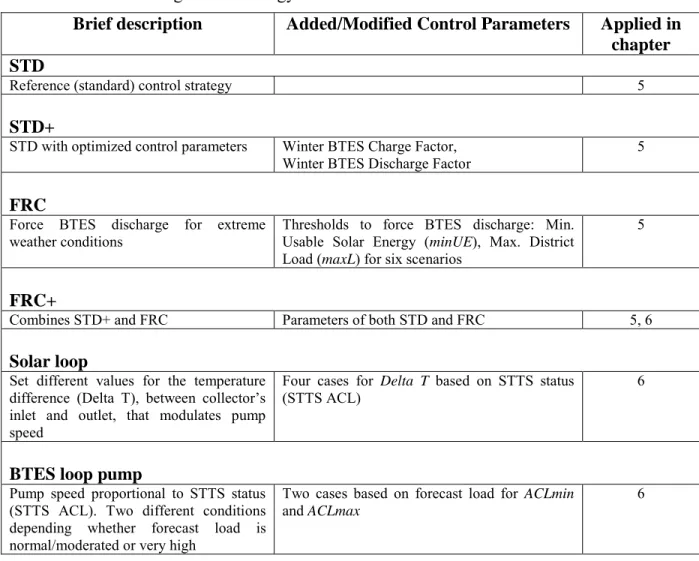
Table 0.1: Control strategies terminology

Brief description Added/Modified Control Parameters Applied in chapter STD

Reference (standard) control strategy 5

STD+

STD with optimized control parameters Winter BTES Charge Factor,

Winter BTES Discharge Factor 5

FRC

Force BTES discharge for extreme

weather conditions Thresholds to force BTES discharge: Min. Usable Solar Energy (minUE), Max. District Load (maxL) for six scenarios

5

FRC+

Combines STD+ and FRC Parameters of both STD and FRC 5, 6

Solar loop

Set different values for the temperature difference (Delta T), between collector’s inlet and outlet, that modulates pump speed

Four cases for Delta T based on STTS status

(STTS ACL) 6

BTES loop pump

Pump speed proportional to STTS status (STTS ACL). Two different conditions depending whether forecast load is normal/moderated or very high

Two cases based on forecast load for ACLmin

(22)

INTRODUCTION

In 2010, residential and commercial space heating accounted for 16% of total energy consumption in Canada and 14 % (66.4 Mt CO2) of the country’s greenhouse gas emissions

(Natural Resources Canada, 2012b). To achieve a significant reduction of these contributions, energy efficiency measures must be supplemented with on-site renewable energy conversion. Solar thermal energy is one of the promising technologies to achieve a high fraction of renewable energy in the built environment, but capital cost represents a significant barrier to its wider deployment in new and existing buildings.

Solar district heating (SDH) systems can deliver economies of scale for equipment and control systems and bring solar heat to individual buildings for space heating and domestic hot water. Unfortunately, solar energy, as other alternative energy sources, suffers a lack of synchronization between demand and supply; more specifically, for space heating the demand is higher during winter months when solar irradiation is lower. A high solar fraction (high share of solar energy in the total heat delivered to the buildings) can only be achieved by using seasonal thermal energy storage – to store the excess of solar thermal energy during summer time – and by the implementation of advanced control strategies for better system management.

The potential of SDH systems and the challenges in implementing them have been recognized by the International Energy Agency Solar Heating and Cooling programme (IEA-SHC), which oversees Task 45, a large Research and Development effort about large solar heating/cooling, seasonal storage and heat pumps “to assist in the development of a worldwide strong and sustainable market of large solar heating and cooling systems by focusing on cost effectiveness, high performance and reliability of systems” (Nielsen, 2012). In Canada, considerable research in the area is supported by the Smart Net-zero Energy Building Research Network (SNEBRN) with its research themes III (Mid-to Long-Term Thermal Storage for Buildings and Communities) and IV (Smart Building Operating Strategies) (SNEBRN, 2013).

SDH systems have been deployed successfully throughout the world with already more than one hundred systems operating in European countries; a complete list can be found in the website of the Solar District Heating (SDH) organization (SDH, 2013). Under the leadership of Natural Resources Canada, the first Canadian system is the Drake Landing Solar Community (DLSC)

(23)

located in Okotoks, Alberta (Wong et al., 2007). The DLSC plant is the case study for this research.

Problem definition

Besides selecting the appropriate component sizes, improving energy performance relies to some extent on an effective supervisory control system designed to manage, among others, the interactions between the Short-Term Thermal Storage (STTS) and the long-term seasonal storage (Borehole Thermal Energy Storage, BTES). In the case of the DLSC control strategy, STTS-BTES control follows an indirect approach for estimating current and near-future heating needs based on current temperature and time of day. Nevertheless, very low ambient temperatures (or a rapid temperature drop), low solar irradiation periods, and low BTES temperatures can lead to cases when the STTS is unable to supply all the needed heat to the district loop.

Another characteristic of the current control is the priority given to solar fraction which basically translates to a diminution of gas consumption. Under some circumstances – related to energy prices and/or CO2 emissions reduction – priority could be shifted to reduce electricity

consumption rather than gas usage.

The paragraphs above lead to the following research questions:

 Can the long-term system performance be improved if the STTS-BTES control strategy is able to anticipate extreme weather events and to adapt the charge/discharge operation accordingly?

 Is it possible for the control strategy to take into account the electricity consumption in addition to the (heat-based) solar fraction so that operating costs (or CO2 emissions if that

is desired) can be optimized?

 Can MPC principles be integrated at different levels in SDH systems (supervisory control, local pump speed control)?

Objectives and scope

The objectives of the project are:

(24)

 Develop new control strategies based on Model Predictive Control (MPC) to increase the energy performance of solar communities and reduce their operating costs.

 Assess the potential of MPC to optimize the supervisory control strategy managing the short-term and long-term thermal storage.

 Assess the potential of MPC to further reduce operating costs by controlling variable speed pumps.

The supervisory control system consists of rules, parameters and set-points for the different system components and fluid circuits. The introduction of new control strategies was limited to the components and circuits being perceived as the ones having a direct impact on reaching the aforementioned objectives.

Methodology

Initial steps consisted of gathering and understanding all possible information about the case study (DLSC); this included articles, reports, schemas, internal documents and most importantly: monitored data for five year of operation and an out-dated – but very useful and instructive – system model implemented in TRNSYS.

The collected documents and data allowed to calibrate the community’s TRNSYS model and to provide the measured weather and heating load to simulations. After this process, potential improvements to the control strategy were identified and alternative controls with predictive features were devised. The method used to build on the existing controller rules and take into account the predicted system behaviour is explained in Chapter 3.

The conceived control strategies were first tested by trial and error to validate their relevance and to identify the control parameters suitable for optimization. In a second step, optimization and tune up of the predictive strategies was performed using measured data as perfect forecasts for weather and heating load. The generic optimization tool GenOpt was employed to evaluate the control strategies parameters that minimize the combined consumption of gas and electricity for different periods of simulated system operation. In the last step, two different MPC approaches were implemented to optimize the control strategies altogether.

(25)

Thesis outline

There are six chapters in this thesis. The first one is a literature review oriented to covering the topics of solar district heating, seasonal storage and control methods, especially Model Predictive Control. The second chapter presents the system used as case study, the Drake Landing Solar Community (DLSC). The third chapter presents the methodology and briefly introduces the proposed control strategies and the concepts applied during the different phases of the project. Chapter four details the process followed to obtain a calibrated TRNSYS DLSC model starting from the original model; this included the development of two new TRNSYS components. Next two chapters introduce and discuss the results of using Model Predictive Control (MPC) for the new control strategies intended to increase overall energy performance during system operation; chapter five describes a control add-on (FRC) that forces the discharge of the seasonal storage in order to have thermal energy more readily available for heating needs; chapter six shows the integration of this add-on with control strategies aimed to reduce pump electricity consumption.

(26)

CHAPTER 1 LITERATURE REVIEW

This chapter describes the concept of solar communities, also known as solar heating districts, and explores the developments for seasonal storage and supervisory control for such systems. Model Predictive Control theory and applications are also especially reviewed to illustrate its potential and limitations.

1.1 Solar Communities / Solar District Heating Systems

A district heating system provides heat from a centralized point to residential or commercial areas to satisfy the demands for space heating and/or hot water. The heat production can be from different sources: gas, biomass, solar, geothermal, co-generation or any combination of them. District heating systems have some advantages over individual heating systems, especially for high density areas or buildings. When using co-generation the energy efficiency of the overall plant is increased due to the utilization of the waste heat for the district (District Heating, 2013). The oldest systems for heat distribution can be traced to the ancient Romans; they used underground tunnels called hypocausts to circulate hot air to heat homes. In modern times, it was in 1877 that the engineer Birdsill Holly conceived the first heating district for Lockport (New York); the system drew a lot of attention and it was soon followed with more plants in the U.S. In Europe, the development of heating districts started as early as 1921 in Hamburg; the system was so successful that by 1938 it was expanded to provide 30 times the initial heat. Similar growth was observed in other countries (Turping, 1966). Nowadays, there are district heating systems in Asian, European and North-American cities, such as the one in downtown Montreal (operating since 1947), which serves 20 large buildings including commercial, residential and institutional customers (Dalkia, 2010).

In the case of solar communities, also known as Solar District Heating (SDH) systems or Central Solar Heating Plants (CSHP), one if the heat sources is obviously the sun’s radiation. The Solar District Heating organization (http://www.solar-district-heating.eu) lists in its European database only the larger plants consisting of more than 500 m2_{of solar collectors’ area.}

The first SDH projects emerged at the end of the 70’s in Sweden, The Netherlands and Denmark. Some of the systems were intended for research purposes so to set the foundations for further projects. In the 90’s, Germany and Austria grew more interested in these kinds of systems and

(27)

more than 100 plants have been built since. In 2010, there were more than 130 SDH systems worldwide, 240 000 m2 of solar collectors, with Sweden and Germany leading. Putting these numbers in context, they only represent 1% of the total of solar collector area installed for solar thermal systems (Dalenback, 2009).

Seasonal Thermal Energy Storage

Short-Term Thermal

Storage Backup Heat

District Loop Supervisory Control Solar Collectors District

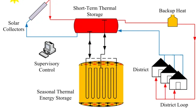
Figure 1-1: SDH system components

The main components of a SDH system are depicted on Figure 1-1:

Heating district: It is the raison d’être of the system. It can consist of individual homes or blocks of apartments. District dwellings are fed with hot water for space heating and/or domestic hot water needs.

Solar Collectors: Capture and transfer solar radiation to a heat carrier fluid which is flowing between them and the short-term storage. In the Northern Hemisphere, to get the best solar irradiation conditions through the year, they are usually oriented towards the south, and tilted the same amount of degrees as the location’s latitude. They can be installed on the roofs or in a separate parcel of land if available. In the latter case, they can also serve other purposes, for example as a sound barrier, as seen in some projects in Germany.

(28)

Short-Term Thermal Storage (STTS): It is a temporary storage of thermal energy coming from the collectors on the way to the users and/or to long-term storage (if available). When heating needs arise in the district, the STTS retrieves thermal energy from the long-term storage when its own state of charge in not enough. The STTS is an optional thermal buffer typically used when the long-term storage exhibits low heat transfer rate or when there is no long-term storage (e.g. systems with a low solar fraction).

Seasonal (long-term) Thermal Energy Storage (STES): It is an optional component that allows increasing solar energy performance by storing the excess of solar energy during the summer and shoulder months to make it available through the winter time. Solar Heating Districts including this component are called Central Solar Heating Plants with Seasonal Storage (CSHPSS). More details about seasonal thermal energy storage will be presented in section 1.2.

Backup heat: It is activated when the temperature of the water going to the district is not enough to fulfill the heating needs. In Figure 1-1 a centralized gas boiler is depicted.

District Loop: It is the heat distribution network that carries hot water to the homes and brings back the colder water to the plant. In some installations it is used as an alternative means of diurnal storage.

Supervisory Control: It is the brain of the plant. It controls the operation by adjusting pumps and valves to transfer thermal energy among the components according to system status and heating needs. Further description and review of the Control component is available in section 0.

1.1.1 Solar Fraction

To quantify solar energy performance in solar districts, the most common measure is the Solar Fraction (SF), usually defined as the ratio between the amount of solar energy delivered to the district and the total energy consumption for district needs. When SDH systems do not have seasonal storage (CSHPxS), or only have diurnal storage (CSHPDS), the SF is usually low (between 10% - 20%), because collected solar thermal energy in winter cannot cope with the increased heat consumption. On the other hand, CSHPSS plants can attain 70% of solar fraction the cases where they are built to provide space heating and domestic hot water (Fisch, Guigas, & Dalenbäck, 1998). Solar fraction can be even higher (more than 90%) for CSHPSS’s designed for

(29)

space heating only (Sibbitt et al., 2012). It is important to mention that initial costs also increase when seasonal storage is considered for the plant.

1.1.2 SDH in Europe

Most solar district heating systems are found in Europe. A complete list is available at the Solar District Heating organization database (SDH, 2013). From that list, a few plants in Denmark, Germany and Sweden will be described shortly. Here, the focus is on those having what is known as Borehole Thermal Energy Storage (BTES), the same type of seasonal storage as used in the case study. BTES details of two of these systems are listed along with the case study in Table 1.1. A review of existing projects in Denmark can be found in Heller (2000). The following comparison shows the evolution of these systems:

Saltum (operates since 1988): With 1 000 m2_{of solar collectors, it is the oldest plant installed in}

Denmark (and one of the oldest in Europe) still operating. Its solar fraction is very low (4%) in part due to the lack of seasonal storage.

Marstal I (since 1996): 18 300 m2_{of solar collectors and diurnal storage. The system reached}

12% of solar fraction before being upgraded.

Marstal II (upgrade in 1998): Includes a Water Thermal Energy Storage (WTES) as seasonal storage. Solar fraction is increased to 25%.

Brædstrup (since 2007, upgraded in 2012): Its collectors area of 18 600 m2 is the largest in Europe. The expected share of heat load is 20% (Brædstrup SolPark, 2012); with a projected BTES storage the target is a long-term solar fraction of 50% (PlanEnergi, 2010).

Information for most of Denmark’s plants, including current status, operational and economic data can be found online at http://solvarmedata.dk.

In the case of Germany, Bauer et al. (2010) compare the most important plants with seasonal heat storage. The installations with BTES storage are:

Neckarsulm (since 1977): 5 570 m2_{of solar collectors and a solar fraction (SF) close to 40%.}

Crailsheim (since 2003): 7 300 m2 of solar collectors. SF is planned to be 50% in the long-term, currently it is 36% (Nussbicker & Druck, 2012).

(30)

In Sweden, the district of Anneberg is operating since 2002. The collector array’s area is 2 400 m2 and seasonal storage is of BTES-type. Solar fraction was projected to be 70% in 5 years (Lundh & Dalenbäck, 2008); however, it has stayed around 40% (Heier et al., 2011).

1.1.3 SDH Worldwide

The case study, Drake Landing Solar Community (DLSC) in Okotoks (Alberta, Canada), with a collector array of 2 300 m2_{and BTES storage, reached more than 95% SF in its 5}th_{year of}

operation (Sibbitt et al., 2012). Chapter 1 gives more details about the case study, its operation and modelling.

Solar heating district projects are not limited to Europe and Canada. In South Korea, a feasibility study for a CSHPSS project in Cheju Island was conducted by Chung, Park & Yoon (1998); more recently, in 2011, a 1 000 m2_{array plant started operations, providing hot water to a}

hospital (http://www.solarthermalworld.org/content/south-korea-hospital-receives-1040-m2-large-scale-collectors).

In China, some cities, including Beijing, are passing laws mandating Solar Domestic Heat Water (SDHW) systems for new residential blocks (of up 12 floors) where no waste heat is employed for heating water (http://www.solarthermalworld.org/content/china-beijing-mandates-solar-hot-water-systems).

In 2012, Saudi Arabia inaugurated what is the biggest solar plant as of March 2013: 36 000 m2 of collectors (almost double as much as Brædstrup) for providing domestic hot water to 40 000 students in the Princess Noura Bint Abdul Rahman University campus in Riyadh

(

http://www.solarthermalworld.org/content/saudi-arabia-worlds-biggest-solar-thermal-plant-operation).

1.2 Seasonal Thermal Energy Storage (STES)

For solar district heating in countries north or south of tropical latitudes, STES is fundamental to overcome the seasonal imbalance between heating needs and amount of solar radiation. With seasonal thermal storage, it is possible to provide in winter some of the heat stored during the summer. In Europe, 21 out of 86 solar heating districts have seasonal storage (SDH, 2013).

(31)

Hadorn (1988) is considered as a seminal reference for seasonal storage; he presents heat storage principles and types along with analytical and numerical methods for modelling and design. The heat storage categories are:

Sensible heat storage: There is no phase change in the substance used for storage, e.g. hot water. It is the simplest and most common way to store heat. All the European plants with seasonal storage listed in the Solar District Heating organization database (SDH, 2013) have some variant of this category.

Latent heat storage: There is a phase change when heat is stored or recovered. They have much higher energy density than the sensible heat type (100-200 times), but their implementation is more difficult due to hysteresis in the phase change cycle and slower thermal energy transfer. A study about using ice slurry as latent storage material can be found in Tamasauskas et al. (2012) Chemical heat storage: Uses reversible chemical reactions where there are virtually no heat losses. The energy density is even higher, – about 10 times that of latent heat storage. There has been some research in the field but no practical applications at district level were found.

The most commonly employed technologies for solar seasonal storage are underground systems based on the principle of sensible heat, using water and/or earth. Pavlov & Olesen (2011) compare and summarize the results from different European CSHPSS systems, with focus in the seasonal storage role. Schmidt et al. (2004) present and define the following types identified in Figure 1-2:

“Hot-water heat storage (also known as Water Thermal Energy Storage-WTES, or simply Water Tank Storage): The water-filled tank construction of usually reinforced concrete is totally or partly embedded into the ground.

Gravel-water heat storage (also known as Water-Gravel Thermal Energy Storage-WGTES or Water Gravel Pit Storage): A pit with a watertight plastic liner is filled with a gravel– water mixture forming the storage material.

Aquifer heat storage (also known as Aquifer Thermal Energy Storage-ATES): Aquifers are below-ground widely distributed sand, gravel, sandstone or limestone layers with high hydraulic conductivity which are filled with groundwater.

(32)

Duct heat storage (also known as Borehole Thermal Energy Storage-BTES): Heat is stored directly into the ground. Heat is charged or discharged by vertical borehole heat exchangers which are installed into a depth of 30 - 100 m below ground surface.”

Figure 1-2: Underground thermal energy storage types (Schmidt et al., 2004. With permission from Elsevier)

ATES and BTES systems cost less but they require additional components (e.g. Buffer storage) and depend on geological conditions (Schmidt & Miedaner, 2012). Roth (2009) stresses the impact of seasonal storage size: storage capacity increases linearly with volume, while thermal losses depend only on area.

1.2.1 Borehole Thermal Energy Storage (BTES)

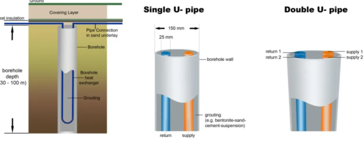
This type of storage uses the ground (soil) as the sensible heat storage medium. It is based on the concept of Geothermal Heat Exchanger (GHX) where a fluid circulating through buried pipe(s) exchanges (delivers or absorbs) heat with the surrounding earth. A typical borehole in a vertical GHX can be seen in Figure 1-3 (left). The pipe(s) inside the boreholes can be placed in different configurations depending on the design (Figure 1-3, right – note that the layout of supply and return pipes can be different). Single U-pipe is the technology employed in Drake Landing.

(33)

Figure 1-3: Vertical section of borehole heat exchangers (left) and common types (right)

In seasonal storage configurations with single U-pipe, borehole pipes are usually serially connected by horizontal pipes from the center to the edge, in order to induce a thermal stratification from the centre to the periphery. The whole storage volume consists of several of these serial branches arrange in a radial way. The charge process circulates water from the center to the edge, making the center hotter than the periphery. During the discharge process the flow is reversed and water from the edge becomes warmer when going through the center (Figure 1-4).

Boreholes

Discharging Charging

Figure 1-4: BTES flow and boreholes connection

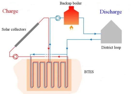
Verstraete (2013) and Verstraete & Bernier (2013) propose and evaluate a double U-pipe storage for solar communities based on the Drake Landing case. As seen in Figure 1-5, there are 2 independent circuits, one connected to the solar collectors for charging the BTES and the other to

(34)

the district loop for the heating load. One of the advantages of this configuration is the absence of a Short-term thermal storage (STTS) leading to simplified control rules.

Figure 1-5: BTES with double U-Pipe (Adapted from Verstraete, 2013)

1.2.1.1 Models

The physical phenomena governing these systems have been studied and modelled by different authors. According to the review by Yang, Cui & Fang (2010) the heat transfer analysis has to consider two regions: inside and outside the borehole. For the heat transfer inside the borehole there are one-dimensional, two-dimensional and quasi-three dimensional models. For conduction outside the borehole, they list the following main models:

Kelvin’s infinite line source (Ingersoll et al., 1950) is the simplest one. It represents the borehole as one infinite line source where only the (one-dimension) radial heat conduction process is considered. The model is very simple and fast to compute but it is limited to applications within short-time intervals.

Cylindrical Heat Source (CHS) (Carslaw & Jaeger, 1959; Ingersoll et al., 1950) models the borehole as an infinite cylinder within a homogeneous medium. The interaction between the

(35)

borehole and the surroundings is also one-dimensional and limited to heat conduction only. This model is more complex to solve and, as the Kelvin’s model, it is less accurate for boreholes operating over long-time intervals.

Finite line source model (Carslaw & Jaeger, 1959) considers the influence of the ground surface as a boundary and approximates the borehole to a finite line source. This model is satisfactory for analyzing the long-term operation of the boreholes.

Eskilson’s model (Eskilson, 1987) introduces more refinement: a numerical model, the spatial superimposition to account for multiple boreholes in the same field, and the non-dimensional g-functions which give the temperature response at the borehole wall for different configurations of the borehole field. The computer implementation requires pre-calculating the g-functions database.

Duct Ground Heat Storage (DST), introduced by Hellström (1989): “The storage volume has the shape of a cylinder with vertical symmetry axis. The ducts are assumed to be uniformly placed within the storage volume. There is convective heat transfer in the ducts and conductive heat transfer in the ground”. The temperature at any point in the ground is obtained from the superposition of three parts: A global temperature process (a heat conduction problem between the storage and the surrounding ground), a local thermal process (around each duct), and a steady-flux part (slow redistribution of heat during injection/extraction). The DST model is implemented in TRNSYS; as a result of calibrating the DLSC TRNSYS model, McDowell & Thornton (2008) found an “excellent [agreement] for both [BTES] charging and discharging operations”. The main limitation of the DST model is that it can only model fields where boreholes are evenly spaced in a configuration that can be approximated by a cylinder (e.g. large square field, but not a narrow rectangular configuration).

To overcome the existing DST model limitations, Chapuis (2009) develops and validates a new model based on the finite-line source method and, spatial and temporal superposition techniques: “it allows the study of borefields where the spatial position of each borehole is defined by the user and where two independent borehole networks can be modeled (one working in charge mode while the other one is in discharge mode, for example)”.

(36)

Bernier, Kummert & Bertagnolio (2007) define and execute a set of test cases to compare CHS, DST, the Eskilson’s model and the Multiple Load Aggregation Algorithm (MLAA) (Bernier et al., 2004) –a technique of temporal superposition based on CHS.

1.2.1.2 BTES installations

The following table compares BTES storage parameters and performance for similar plants. Table 1.1: BTES comparison for different SDH systems

Drake Landing-Okotoks, year 5 (Sibbitt, 2012) Anneberg, year 5 (Heier et al., 2011) Crailsheim design (Nussbicker & Drück, 2012).

Number of dwellings 52 50 260 + school and

gymnasium Application Space heating Space heating and

domestic hot water Space heating and domestic hot water

Volume (m3₎ _{35 000} _{60 000} _{37 500}

Number of boreholes 144 100 80

Deep of boreholes (m) 35 65 60

Short-term Storage (m3) 240 0.75 – 1.5/sub-unit 480

Heat pump No No Yes

Total heat demand

(MWh/yr) 588 565 4 100

Collected Solar Energy

(MWh/yr) 1 230 1 075 2 700

Energy delivered to

BTES (MWh/yr) 700 720 1 135

Energy extracted from

BTES (MWh/yr) 252 333 830

1.3 Supervisory Control

The objective of supervisory control for buildings is to keep a balance among occupant comfort and energy conservation. A review of control systems for building environment by Dounis & Caraiscos (2009) includes legacy technologies such as thermostats and PID controllers (proportional - integral – derivative); more elaborate methods using Computational Intelligence (CI) (fuzzy logic, neural networks, evolutionary algorithms, etc.); and Model-based Control strategies: optimal, predictive and adaptive. According to Clarke et al. (2002), Model-based control should be preferred to CI; the latter need a training period, they ignore the physical

(37)

underlying system phenomena and their control decisions are not tractable. Another advantage of Model-based control is that it is better suited to be considered during the early stages of building design as it is proposed by Petersen & Svendsen (2010).

Henze, Dodier & Krarti (1997) present three conventional thermal storage control strategies for cooling applications in buildings: chiller-priority, constant-proportion and storage-priority. They state that some of these can also be applied for other types of thermal storage. The first 2 methods are mainly based in current system and weather conditions, but storage-priority implies some level of load prediction. More advanced methods, such as optimal control, allow taking advantage of the passive building thermal storage to time-shift peak electrical load and reduce electricity costs (Braun, J., 1990). De Ridder et al. (2011) describe a dynamic programming algorithm for a long term storage coupled to a heating, ventilation and cooling (HVAC) system. For the general case of district heating systems, Saarinen (2008) explains how the common method for controlling supply temperature, called Feed-Forward Control, can be improved by using a dynamic algorithm for load prediction.

1.3.1 Control for Solar District Heating

The design of the control system for a SDH plant always meets “conflicting targets” as enumerated by Schubert & Trier (2012): “Avoidance of stagnation of the solar system, optimal use of heat storages, minimization of heat losses in collectors, pipes and storages; minimal electricity consumption of pumps, minimum requirement of human intervention, optimal use of other heat sources like heat pumps, boilers, waste heat”

This is confirmed by Wong et al. (2007) regarding Drake Landing: “Optimizing the control strategy was a significant challenge, developing into a balancing act between the two primary goals of assuring occupant comfort and maximizing the solar fraction.”

In a SDH plant with no seasonal storage, there are mainly two circuits to control: the charge circuit which includes the collectors and the short-term storage, and the discharge circuit (of the short-term storage) for supplying heat to the district. In the charge segment, the concept of variable flow rate is applied to the circuit pump whether using collector temperature

measurement or collector irradiation measurement (Schubert et al., 2012). The Marstal plant

(38)

modulating the pump speed to maintain a predefined temperature difference between the solar collectors’ inlet and outlet ports (Wong et al., 2007).

The short-term thermal storage (STTS) discharge circuit is activated when the district demands thermal energy from the plant. According to Wong et al. (2007), “the biggest challenge with the District (discharge) Loop was to ensure the greatest temperature drop through the system”, this ensures “efficient operation of the STTS by maintaining stratification” and increases the “efficiency in the solar collectors by maintaining the lowest inlet water temperature.”

When there is a seasonal storage, two additional circuits, for its charge and discharge, need to be controlled. The seasonal storage is mainly charged from the STTS during summer, besides building the thermal energy reserve, another objective is to make sure that the short-term storage is able to collect the daily solar radiation. The discharge is essentially started for winter periods where the buffer storage has not enough charge to conveniently feed the district loop. No detailed information was found about how these processes are controlled in plants other than Drake Landing; this case will be described in Chapter 2.

1.4 Model Predictive Control (MPC)

As its name states, this control method is based on a model of the actual physical system and predictions of external conditions (or disturbances). With these two elements, MPC is able to determine the best control input to the system so its output is the closest as possible to the expected output.

The following MPC theory is based on the book by Rossiter (2003). The initial concept is that a system model can be represented using the concept of transfer function or state-space matrices. The latter representation is preferred because it is more convenient and less complicated than the former one for the cases of multiple-input, multiple-output (MIMO) systems. In the case of a Linear Time Invariant (LTI) system the state-space matrices (A, B, C, D and F) are constant – because there is no time dependency– and the model is given by

x(k+1) = Ax(k) + Bu(k) + Fd(k) (1.1)

(39)

where, x is the state vector, y is the system’s outputs vector, u vector is the controller input to the system, d is the disturbances vector, and (k, k+i) indicate consecutive discrete time samples – commonly used in MPC applications. Future system status and outputs can be predicted for each time sample over a horizon of length p by using the above equations on a recursive fashion:

x(k+2) = Ax(k+1) + Bu(k+1) + Fd(k+1) = A(Ax(k) + Bu(k) + Fd(k)) + Bu(k+1) + Fd(k+1) y(k+2) = Cx(k+2) ... x(k+p) = Apx(k) + Ap-1Bu(k) + Ap-2Bu(k+1) + ... + Bu(k+p-1) + Ap-1Fd(k) + Ap-2Fd(k+1) + ... + Fd(k+p-1) y(k+p) = C•_x(k+p) (1.3)

What equations 1-3 mean is that the system’s output at the time sample k+p can be predicted by using the system’s state at the current time sample (x(k)), the accumulated control inputs (u(k) to u(k+p-1)) and the predicted disturbances for the horizon (d(k) to d(k+p-1))

If the expected system’s output for any time sample is written as ŷ(i), the difference between the actual output and the expected output is e(i) = ŷ(i) - y(i), and a control performance index over a the period can be written as :

J = ∑ || e(i) ||2 + ∑  ||∆u(i)||2 ; i=k+1 to k+p (1.4) where, is a weight factor to account for big changes in u.

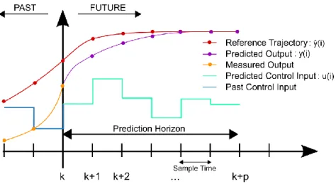
Applying MPC consists in solving equations 1.3 to find the optimal control for each time sample (u(i)) so the performance index or cost function J is minimized. In other words, the optimization algorithm considers predicted disturbances (d) and system’s output to determine the set of control inputs that would allow the system to reach the intended output or reference trajectory (ŷ) over the entire prediction horizon (Figure 1-6). At each iteration, only the first calculated control inputs (u(k+1)) are applied to the real system and a new optimization for the next time sample is performed taking into account the resulting system’s state and updated disturbances forecasts. The period (p) over which the control inputs are estimated is called receding horizon because it keeps moving forward after each iteration so it is never reached.

(40)

Figure 1-6: Model Predictive Control by Martin Behrendt (2009). Made available under Creative Commons Licence.

1.4.1 Online and offline MPC

1.4.1.1 Online MPC

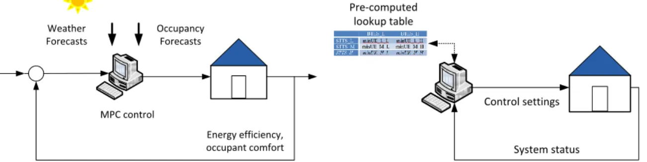
The general MPC description is also known as online MPC; it is called this way because the physical system and the model-based control are tightly coupled. Figure 1-7 illustrates how MPC control continuously takes the decisions for modifying control settings based on feedback from the actual system and disturbances forecast.

Weather Forecasts Occupancy Forecasts Energy efficiency, occupant comfort MPC control Figure 1-7: Online MPC

(41)

There are multiple MPC variants with different optimization algorithms but all of them share the main features: being based on a model of the actual physical system, computing the control signal using disturbances prediction and the receding horizon concept (Maciejowski, 2002); e.g., Robust MPC controllers account for model and/or disturbances uncertainty (Jalali, 2006).

Applying optimal control one interval at a time and then using the system output to repeat the process is called Closed-Loop Optimization (CLO). This is not the only way of implementing MPC, another approach is Continuous Time Block Optimization (CTBO) (Henze et al. 2004). It is different from CLO because the whole block of optimal control values found for the period is applied to the system. In this approach the next optimization is done for the period starting in k+p. Figure 1-8 compares the two options using (purple and blue) solid lines to indicate the extent of the optimal control input applied in each case.

CLO CTBO Figure 1-8: CTBO and CLO

1.4.1.2 Offline MPC

As an alternative to online MPC, the concept of offline MPC can be employed for certain situations when either online MPC is not feasible and/or its computation time is very high. In this variant, there is no control parameters being calculated in every time interval, instead a lookup table for a grid of system scenarios is pre-computed using simulation software (Coffey, 2012). The table contains the values of optimal control parameters for each scenario which are found after following an optimization process. When the real system is found to be in a particular status –represented by a cell of the grid– the specific parameters are then employed to control the

(42)

system without running any additional simulation (Figure 1-9). To apply the concept of lookup tables the optimization problem is simplified by using problem decomposition and conditions parameterization (Coffey, 2012). Pre-computed lookup table System status Control settings Figure 1-9: Offline MPC

1.4.2 MPC research and applications

Using Model Predictive Control for buildings is already proposed by Kelly (1988), but the intensive computation power required for the calculations limited its development. There are some early works by Braun (1990) focusing on controlling cooling systems and building thermal mass, and Camacho et al. (1994) for controlling solar collector fields.

With increasing and less expensive computing power, there have been more research works in this field: a predictive optimal controller for thermal storage (Henze, Dodier & Krarti, 1997), validation and test for a passive solar building (Kummert, 2001), a review of MPC potential and challenges (Coffey, Morofsky & Haghighat, 2006), MPC for controlling a geothermally heated bridge (Xie & Whiteley, 2007), a comparison between MPC and PID control for a single solar system (Ferhatbegovic, Zucker & Palensky, 2011), MPC and weather forecasts for controlling a building temperature (Oldewurtel et al., 2012), Predictive control for buildings with thermal storage (Ma et al., 2012).

It is also worth mentioning the ongoing European interdisciplinary project OptiControl (www.opticontrol.ethz.ch) presented as the “Use of weather and occupancy forecasts for optimal building climate control.” Simulation results indicate a theoretical energy saving potential of 1% to 15% for non-predictive algorithms and up to 41% for predictive control algorithms depending

(43)

on the location, building case, and other parameters (Gyalistras, 2010). The companion website www.bactool.ethz.ch allows online access to the Building Automation and Control Tool (BACTool) for graphical evaluation of different control algorithms.

Improving MPC results is clearly dependant on accurate forecasts. Florita & Henze (2009) compare and evaluate different weather forecast models for MPC applications, especially those based on Moving Average (MA) and Neural Networks (NN). They found that for MPC applications, MA models, in spite of their simplicity, are often better than complex NN models at predicting outside temperature. For solar irradiation forecasts, Perez et al. (2007) evaluate a model to produce finer forecasts using information from simple sky cover predictions, Cao & Lin (2008) define and compare the accuracy of a proposed type of Neural Network, called Diagonal Recurrent Wavelet Neural Network (DRWNN). In 2010, Perez et al. present a validation, against ground measurements, of the algorithms employed by the US Solar Anywhere system (solaranywhere.com). IEA, task 46, “Solar Resource Assessment and Forecasting”, also points in this direction. In another kind of forecasting, Mahdavi et al. (2008) explore the usage patterns and profiles of office building occupants to facilitate the operation control.

No comprehensive research for applying Model Predictive Control strategies for SDH was found; articles refer to particular or local control problems. In an IBPSA workshop about MPC, Candanedo (2011) presents models for individual house heat loads and solar gains at the community scale, and he also summarizes some results of the “effect of imperfect solar gains forecasts on predictive control”. Some other works more related to general district heating can be found, for example, application of predictive control for district heating to keep a low district supply temperature (Palsson, Madsen & Søgaard, 1993); Dobos et al. (2009) uses the Matlab toolbox for applying MPC in different local problems of a heating district. Sandou (2009) states that the Particle Swarm Optimization (PSO) algorithm for predictive control gathers better results than classical control rules for heating districts.

1.4.3 Software

To solve an optimization problem using MPC, two main software processes are needed: simulation and optimization. For building applications, simulation software such as TRNSYS (Klein et al., 2012), EnergyPlus, or ESP-r, are widely employed for system modelling and simulation. For optimization, the program GenOpt (Wetter, 2001) easily integrates with

(44)

simulation software through input and output text-files. Matlab also provides an MPC toolbox but it requires the system to be defined in terms of the transfer function or a state-space model (www.mathworks.com/products/mpc/). The optimization program evaluates the simulation’s output and applies special algorithms to find the control parameters values that minimize a defined cost function, which should corresponds to the best point of system operation.

(45)

CHAPTER 2 CASE STUDY: DRAKE LANDING SOLAR COMMUNITY

(DLSC)

2.1 Description

The SDH plant at Drake Landing Solar Community provides solar space heating for 52 homes. The community is located in the town of Okotoks (Alberta, Canada) at 50° latitude North and 1000 meters above sea level. It is the first district with solar seasonal storage in North America and the first in the world to reach a 90% solar fraction.

The community was designed in 2003 by a team led by Natural Resources Canada (NRCan) following an initiative to apply the concept of solar energy and seasonal storage for sustainable communities. The project’s success is testimony to the commitment of NRCan and its multiple partners, including the municipality and private companies, such as Sterling Homes and ATCO Gas.

Construction started in 2005, after some delays and unexpected expenses it was set in operation two years later. Distributed sensors monitor the system and performance reports are generated monthly and yearly. After three years of operation, solar fraction was already 80%. At the end of year 5 (July 2012), solar fraction reached 97% (Sibbitt, 2012), surpassing the design values. In 2011, the community was awarded with the prestigious Energy Globe Award in the Fire (Energy) category and the overall World Energy Globe Award. Countries like South Korea are also considering similar communities based on the learning from this experience (Patterson, 2012); the same article indicates that “The [DLSC] project’s partners are now looking at taking the technology to the next level by developing a large-scale solar community with between 200 to 1,000 homes”.

2.2 Components

The excellent energy performance observed in this plant is mainly the result of a careful design; components characteristics were defined to maximize solar energy collection and storage, and to minimize heating load. On one side, these considerations apply for the centralized solar plant equipments; on the other, they translate in better homes’ insulation and very efficient air handler units. As objectives are not only related to energy performance but also to sustainable

(46)

development principles, material and supplies were chosen according to special criteria, such as certified lumber source, local manufacturing, and recycled sources.

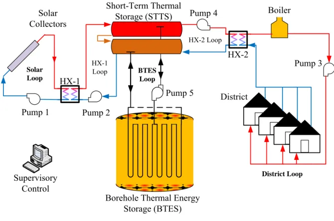
The main components of the plant and circuits (fluid loops) that connect them are depicted in Figure 2-1. Their characteristics are extracted from (McClenahan et al., 2006), (Wong et al., 2007) and Drake Landing’s website (http://www.dlsc.ca). Heat exchangers, pumps, boilers and short-term storage tanks are installed in a building called the Energy Centre. BTES storage is underneath an adjacent park.

Borehole Thermal Energy Storage (BTES) Short-Term Thermal Storage (STTS) Boiler District Loop Supervisory Control Pump 1 Pump 2 Pump 5 Pump 4 Pump 3 HX-2 HX-1 Solar Collectors District Solar Loop HX-1 Loop HX-2 Loop BTES Loop

Figure 2-1: Drake Landing Main Components

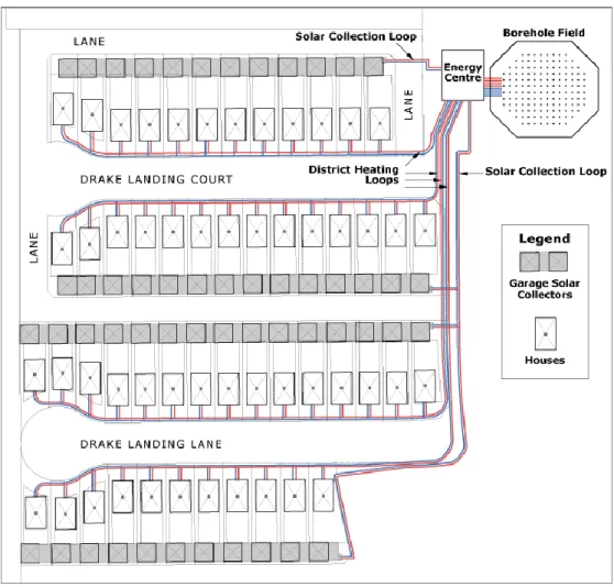
Solar collectors: There are 798 flat-plate collectors oriented towards the south and tilted 45° above the horizontal. Each one measures 2.45 m x 1.18 m; the whole array covers an area of 2293 m2. Mounted in the garages’ roofs, they are grouped in 4 blocks following the community’s layout of four rows of houses (Figure 2-2). The heat carrier fluid circulating through them is a mix of glycol and water.

(47)

Figure 2-2: Drake Landing layout (Source: http://www.dlsc.ca, retrieved May 15, 2013)

Heat Exchanger 1 (HX-1): it allows heat transfer from solar collectors to the Short-Term Thermal Storage (STTS). When collectors are hot enough, heated glycol circulates through HX-1 transferring heat to water in the HX-1 loop. Cold glycol returns from HX-1 to the collectors’ inlet to reinitiate the sun’s energy transfer cycle.

Pumps 1 and 2: They are variable speed pumps. Pump 1 circulates the glycol in the solar loop. At the same time, Pump 2 circulates water in the HX-1 loop. For backup purposes, both pumps are duplicated.

Short-Term Thermal Storage (STTS): it consists of two 120 m3 _{tanks, totalizing 240 m}3_{. The first}

tank (hot tank) receives hot water directly from HX-1. The bottom outlet of the hot tank is connected to the top inlet of the second tank (cold tank). Closing the loop, cold tank returns cold

(48)

water to HX-1. For improved stratification, each tank has an internal division by means of a special baffle.

Figure 2-3: BTES distribution (Source: http://www.dlsc.ca, retrieved March 22, 2013)

Borehole Thermal Energy Storage (BTES): It is composed of 144 boreholes of 15 cm diameter and 35 m deep, separated 2.25 m from center-to-center. Each borehole contains a single U-tube. These pipes are serially connected in strings of 6 from the center to the edge for better radial stratification. Four circuits made up of non-adjacent strings increase reliability of water supply and return (Figure 2-3). The total earth volume is 35 000 m3_{, and the equivalent water thermal}

capacity is 15 800 m3_.

Pump 5: It is the pump for BTES charge and discharge operations. The pump is actually unidirectional, with the flow direction dependant on the position of the BTES loop valves determined by the control platform. Two constant speed pumps in standby-backup configuration were initially installed for this operation, but a variable speed pump was retrofitted in 2012. Heat Exchanger 2 (HX-2): Transfers heat from STTS’ hot tank to the district loop when heat demand exists. The HX-2’s outlet in the small HX-2 loop is the return path for cold water to STTS’s cold tank.