Applied Plasma Research

IX. APPLIED PLASMA RESEARCH

A. Active Plasma Systems

Academic and Research Staff

Prof. L. D. Smullin Prof. R. R. Parker Prof. R. J. Briggs Prof. K. I. Thomassen

Graduate Students

Y. Ayasli R. K. Linford J. A. Rome

D. S. Guttman J. A. Mangano M. D. Simonutti

1. STABILITY OF ELECTRON BEAMS WITH VELOCITY SHEAR

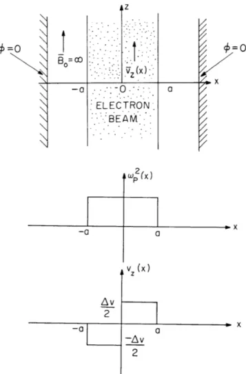
We have expanded our study of cold, slab electron beams that are focused by infinite longitudinal magnetic fields to encompass the step velocity profile case. Throughout, we assume that w is a constant independent of the cross-sectional position x.

Further-p

more, we have worked in a frame of reference in which the average electron velocity is zero. The complete geometry is illustrated in Fig. IX-1.

It is obvious at the outset that this case is closely analogous to the familiar "two-stream" instability, and hence we might expect similar results. In particular, in the long-wavelength limit, with zero potential walls far from the stream edges, the poten-tial will be essenpoten-tially constant across the stream and hence the two streams will not

be able "to tell" whether they are adjacent or intermixed.

This problem was studied in 1963 by Harrison and Stringer. They concluded that these profiles are unstable for large enough velocity differences, but their instability conditions are quite different from ours because theirs are independent of stream width.

In general, for arbitrary velocity and density profiles, the potential is the solution of the differential equation2

2

2 p (x)

d k2 2 = 0,

(1) dx [u-v (x)]2

where we assumed solutions of the form (x) exp(i(wt-kz)), and u = W/k is the phase velocity. To test for instability, we assume that k is real and look for w (or u) with negative imaginary parts. In each region of the beam the solution is sinusoidal, and hence we may easily derive a determinantal equation by forcing p and d4/dx

2 w

(X)

vz (x)

Av

2

-a

-Av

2

Fig. IX-1. Geometry of the step-beam.

to be continuous at the interfaces.

We have found the equations for two particular

cases.

I.

Zero-Potential Walls at the Beam Edges

D(u, k) = (kxla) cos (kxla) sin (kx2a) + (kx2a) cos (kx2a) sin (kxla).

II.

Zero Potential Walls at x

=

+oo

D(u, k) = kxl

a[(ka) sin (kx2a) + (kx2a) cos (kx2a)][(kx1a) sin (kxl

a) - (ka) cos (kxla)]

+ kx2a[(ka) sin (kx

a) + (kx

a) cos (kxla)][(kx2a) sin (kx

a) -(ka) cos (kx

a)],

(3)

where

0=o

(IX. APPLIED PLASMA RESEARCH)

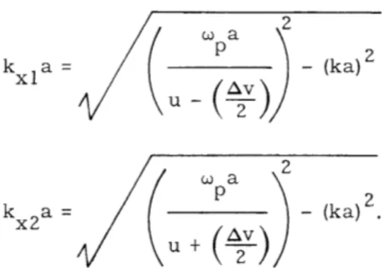
kxa= ( - (k a )

2

/

₂

kx2a=

x 2

K2

The roots of these equations yield the values of u and k that can exist on the beam. The task of finding the complex roots of these equations is performed by a digital computer. Fortunately, we can prove that all of the unstable roots of D(u, k) must lie on or in the semicircle in the lower half u-plane defined by

1

2

1

i

ur

-

as is illustrated in Fig. IX-2. The minimum and maximum electron velocities in the beam are v min and v max. The proof of this is patterned after a similar fluid mechanics

Uimaginary

u - plane

Vmin) Vmax

Ureal

1/2 (Vmax-Vmin)

Fig. IX-2. Geometry of the semicircle theorem.

3 *

theorem. It consists in multiplying Eq. 1 by

4

Since the roots of D(u, k) must lie in a restricted portion of the u-plane, we can use a Cauchy integral technique to find the locations of all roots in this region. This tech-nique, formulated by J. E. McCune and B. D. Fried, uses the fact that

N P b

n. z

zj

i=l

j=l

C

f(z)

where C is any simple, closed curve of finite length in the z-plane enclosing N zeros zi

of order n

and P poles zj of order pj.

For instance, if b

=

0, the left-hand side of

Eq. 5 yields N- P; if b

=

1, it yields Z n.z.

-

f p.z

and so forth. These equations

may be solved simultaneously to find the orders of the poles and zeros and their

loca-tions.

The program for calculating this complex line integral was written by James D.

Callen

and was used successfully in the present study. As is to be expected from

anal-ogy with the two-stream situation, the onset of unstable roots occurs for the real part

of u

=

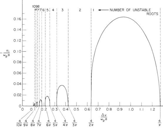
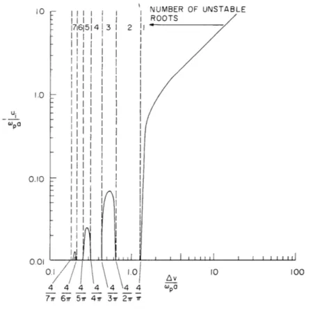
0. Figures IX-3 and IX-4 are plots of the imaginary part of u/w a against Av/Wpa.

Only those roots with real (u)

=

0 are shown.

Also shown are the total number of roots

in each range of Av/w a, those not shown being complex and lying inside the semicircle.

In Figs. IX-5 and IX-6,we show normalized w-k diagrams for fixed Av/w a. All modes

P

are stabilized for large enough ka.

The case with walls at the beam edge shows a definite lower density limit below

which the instability ceases.

On the other hand, when the walls are moved to infinity,

1098 I 1i176 5 4 3 -

~

Fig. IX-3.

-u./w a vs Av/w a for the step beam with walls at edges

for ka

=

0.

(Only purely imaginary roots are shown.)

ui pa 0.16 0.14 0.12 0.10 0.08 0.06 0.04 0.02

1_1 ~ 1

1

I

1

(IX. APPLIED PLASMA RESEARCH)

I

I

K'flf

|

'I

I

Fig. IX-4.

-ui/w a vs Av/w a for the step beam with walls at infinity

for ka

=

0.

(Only purely imaginary roots are shown.)

a mode persists even down to zero density for which u.

=

-Av.

Figures IX-7 and IX-8

show the analogous case for the conventional interstreaming-beam situation where

the number of electrons traveling at each velocity has been maintained for

compar-ison purposes.

There is fairly close agreement between the adjacent beam and

inter-streaming beam cases, except that the adjacent beam case has some complex roots that

do not occur in the conventional two-stream case.

All plots have their maximum

value of u. I when k

=

0.

Furthermore, as k is increased, the various modes are

stabilized.

The onset of instability for each mode can easily be predicted because, for u

E

0,

k

_xl

= kx

_x2

_A

-

(ka)

.

Also, assume ka = 0.

In these limits, Eqs. 2 and 3

both become

D(u, k)

=

cos (

/

sin

2w

.

(6)

Thus, the neutral k = 0 modes occur when

u

i

Wpa

0.10

0.10 0.08 0.06 0.04 0.02 0 0.2 0.4 0.6 0.8 1.0 1.2 1.4 1.6

Fig. IX-5. -. i/w_p vs ka for the edge for Av/W a = 0.

0.06 0.05 0.04 0.03 0.02 0.01 F

step beam with walls at

90.

0 0.2 0.4 0.6 0.8 1.0 1.2 1.4 1.6

ka

vs ka for the step beam with walls at infinity

for Av/w a = 0. 52.

is shown.)

(Only the purely imaginary root

0.16 0.14 0.12 0.10 0.08 0.06 0.04 0.02 0 0.1 0.2 0.3 0.4 0.5 0.6 0.7 0.8 0.9 1.0

Fig. IX-7. -u./w a vs Av/w a for

'p

p

U

i

Wpa

edges for ka = 0.

the interstreaming beam with walls at

0 0 1 0.2 0.3 0.4 0.5 0.6 0.7 0.8 0.9 1.0 1.1

Av

Wp(

Fig. IX-8.

-ui/w a vs

Av/w a for the interstreaming beam with walls at

P

Av 4

Sn

= 1, 2, 3, ....

(7)

wa

In conclusion, we find that the adjacent-stream case exhibits a two-stream instability that is very similar to the conventional interspersed-stream case. When zero-potential walls are at the beam edges, there is a definite onset of instability at p a > iAv/4. The minimum density case occurs at k = 0. If the walls are at infinity, there is a mode that does not exhibit a density threshold. Contrary to the interspersed case, there are com-plex (not pure imaginary) values of o for real k in addition to the pure imaginary values shown here.

J. A. Rome, R. J. Briggs

References

1. E. R. Harrison and T. E. Stringer, "Longitudinal Electrostatic Oscillations in Velocity-Gradient Plasmas. II. The Adjacent-Stream Mode," Proc. Phys. Soc. (London) 82, 700 (1963).

2. R. J. Briggs and J. A. Rome, "Stability of Electron Beams with Velocity Shear," Quarterly Progress Report No. 90, Research Laboratory of Electronics, M. I. T.,

July 15, 1968, pp. 106-107.

3. P. G. Drazin and L. N. Howard, "Hydrodynamic Stability of Parallel Flow of Invis-cid Fluid," Advances in Applied Mechanics 9, 62 (1966).

4. J. E. McCune and B. D. Fried, "The Cauchy-Integral Root-Finding Method and the Plasma 'Loss-Cone' Instability," Report CSRTR-67-1, Center for Space Research, M.I.T., January 1967.

5. J. D. Callen, "Absolute and Convective Microinstabilities of a Magnetized Plasma," Report CSR TR-68-3, Center for Space Research, M. I. T., April 1968.

IX.

APPLIED PLASMA RESEARCH

B.

Plasma Effects in Solids

Academic and Research Staff

Prof. A. Bers

Prof. G. Bekefi

Dr. E. V. George

Graduate Students

R. N. Wallace

1. MODEL FOR THE MICROWAVE EMISSION FROM THE

BULK OF n-TYPE InSb

Our recent experiments on the microwave noise emission from the bulk of n-type

InSb at 77°K in applied crossed electric and magnetic fields show two important

fea-1

tures

:

(a) the emission originates from localized regions of the material; and (b) the

thresholds of electric and magnetic fields are higher than those found in samples with

"bad" contacts.2

From these results, we conjecture that the emission is related to

inhomogeneities in the material. Metallurgical studies

show that in most InSb crystals

inhomogeneities in the impurity density occur in 1-10 [ regions.

The detailed nature

of these inhomogeneities is unknown, but it is clear that the electric field in regions of

lower electron density would be higher (perhaps by a factor of 2-4) than the average

applied field.

Furthermore, as we shall show, in the presence of a transverse magnetic

field the rate at which electrons gain energy from the electric field is also enhanced.

Taken together, these two effects predict that a fraction of the current will produce

charge multiplication in localized regions, and we can compute the resultant shot-noise

generated.

We shall summarize the analytical results of this model and compare them

with our observations.

Energy Gained by Electrons in Crossed Electric

and Magnetic Fields

This problem has been treated in the past phenomenologically for predicting

total-current breakdown in a strong Hall electric field.

Our interest is in a more detailed

description of the electron energy gained from the total electric field (applied field and

Hall field), since only a small fraction of the current is considered to produce

break-down. Hence we start with the time-independent Boltzmann equation for the electron

distribution function f(v, E,

B)

in electric and magnetic fields E and B,

e

f

(E + vXB) • V-f= -

(1)

m (e) T(E)

where we have assumed a relaxation-time approximation for the collisions and (E) energy-dependent effective mass m and relaxation time T. We separate f into its isotropic and anisotropic parts

f = f. + f ₍₂₎

1 a

from which the current is given by 2fv

-va

where n is the electron density. Substituting Eq. 2 in Eq. 1, we can solve for f in

5 a terms of f. 1 df. (E + TW X E) 1-f =-eT v c (4) a d (

2

where we have assumed that E is perpendicular to B and the anisotropic part of (E V f a ) is negligible, and have written c = Be/m. Using Eq. 4 in Eq. 3, and letting B=izBo, E= ixE + iEy, we find

7 T/m c T 2/m 1 - /E E - (5)

c

c

F

J=eE+

,6

y

L

T

where the brackets indicate the following average over the energy distribution function

(X)

=

E

1 E

Consider now that the applied electric field E is in the x direction, and the o

geometry is one of zero Hall current, J = 0. The Hall electric field is then given by

y

(IX. APPLIED PLASMA RESEARCH)

/m

Y

22

S-HEo.

(8)

Our interest is to determine the energy gained by an electron of a particular energy from both the applied and Hall electric fields. The "drift" velocity of an electron of a particular energy, v(E), may be found from Eqs. 5 and 6 by dividing them by (en) and removing the brackets. Then, using Eq. 8 for Ey, the power input to an electron of a particular energy is PI(E) e v(E) " E 2 1+ 2

eT

HE

(9)

c

where T and m are energy-dependent.

Charge -Multiplication and Shot-Noise Generation

In order to determine the conditions for the onset of local breakdown, we must com-pare the energy-gain rate of Eq. 9 with the energy-loss rate. The energy-loss rate to optical phonons is given by hw /Te, where w is the optical phonon frequency, and Te is the electron energy relaxation time. An electron starting from an energy E may gain energy and produce an ionizing collision, provided PI exceeds ihwo/T e for energies from E to above the energy gap E .

Figure IX-9 is a plot of the normalized energy gain and loss rates, PI/E and 2

hWo/TE , as a function of electron energy. In making this plot, we have used known 6

data for the variation of the effective mass with energy, and theoretical formulas for the electron momentum and energy scattering times in interactions with optical pho-ons.7 An average momentum scattering time of 4 X 10-12 s, deduced from the low-field electron mobility, was used for electron energies less than hw . We note that for suf-ficiently small values of E and Bo no electrons satisfy the condition PI > Tiwo/ e. As E and Bo are increased, PI eventually exceeds lioo/Te for energies from some value Ea < Eg through energies above Eg. The fraction of the electrons having energy greater than Ea can gain energy from the total electric field to produce ionizing collisions. Thisa

"ionizing fraction," F, of the electron population can be computed by assuming an

appropriate Maxwellian distribution, which we shall describe.

2 PI /E SE=0 V/cm -2 E =50 V/cm 10-16 5 2 IO _1 3: ---0 o - 18 01 Bo=10.0 kG 6.4 3.2 S3.2 O 2 4 6 8

C/hw

Fig. IX-9.

Normalized energy gain and loss rates per electron as a function

of the electron energy in optical phonon units for various values

of E and B .

(E is the local value of the applied electric field.)

o

The conditions in a typical inhomogeneity region of an InSb crystal are then

considered.

From the known order of length of the inhomogeneity region we find

that each electron in the "ionizing fraction" creates, on the average,

one additional

electron-hole pair.

These generated carriers give rise to a shot-noise-producing

current which is approximately FI ,

where I

is the drift current in the sample.

The inhomogeneity region can then be thought of as a localized microwave

cur-1/2

rent source of rms value [2eFI (Af)]

,

where Af is the receiver bandwidth.

In

our experiments,

this localized current source, together with the loop sample

forms a driven antenna system that excites the eccentric transmission line. The

power coupled from this "antenna"

to the eccentric transmission line can then

be computed directly.

(IX. APPLIED PLASMA RESEARCH)

Comparison with Experiment

The power delivered to the receiver is proportional to

f

Ta Tis

the magnetic field mode function for our eccentric transmission line, A is the cross section of the line, and J is the microwave current density distribution on the loop

a

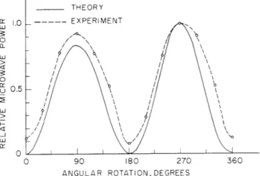
sample as determined above. From this, we can calculate the output power as a func-tion of sample rotafunc-tion and compare with our experimental results. This is shown in

Fig. IX-10 for a sample that showed a marked variation in output with sample rotation.

Q 1.0 0 a-0

o

ANGULAR ROTATION, DEGREES

Fig. IX-10. Comparison of theoretical and experimental variation of microwave power with sample rotation, with Bo perpen-dicular to the sample plane. Frequency = 9 GHz.

We conclude that our model of a localized source is indeed supported by experiment. We next turn to a more detailed test of our model in which we seek to predict the observed Eo -B threshold curve and the output power at threshold (Fig. IX-11). The two principal unknowns in our model are the electric field in the inhomogeneity region (which may be M times larger than the nominal applied field Eo) and the electron energy distribution function. The first affects the actual electric field (Eq. 9) and the second enters into H' both then determining Ea (Fig. IX-9) and thus the Bo vs Eo dependence of the ionizing fraction F. We shall initially assume that M is in the range 2-4, and that the electron distribution function is a two-temperature Maxwellian with different temperatures above and below the optical phonon energy.9 The electrons in the main body of the distribution (E < hiw₀ ) essentially determine cH, while the electrons in the high-energy tail (E > hw ) will affect the detailed magnitude of F. When acoustic phonon

scattering determines the main body of the distribution function, it can be shown5 scattering determines the main body of the distribution function, it can be shown5 that

in moderately high electric and magnetic fields (\E/va

>>

w

>> 1, where v and

are

the acoustic velocity and scattering time) the isotropic part of this distribution, f., is

55 5.0 EXPERIMENTAL POINTS Bo(kG) 40 3.0 -O 08 H/ HO 0 10 20 30 40 E0(V/cm)

Fig. IX-11.

Experimental values (dots) of electric and magnetic

field required to maintain a constant threshold

(min-imum detectable) emission level equivalent to that of

a thermal source of 0. 5-1.0 X 103 K at 9. 0 GHz.

The

-1

theoretical model with 'H ~ Eo predicts the observed

threshold fields and gives the observed emission power

level if the electron distribution tail temperature varies

as E

0

THEORET

2

approximately Maxwellian with an electron temperature that increases as E . Adopting

-O

this for electrons below the optical phonon energy leads to H ~ E . We can then deter-mine the tail temperature which gives the output power level observed on the threshold curve (Fig. IX-ll11). We find a tail temperature that increases approximately as E , and hence remains at a lower temperature than the main body of electrons.10 Our calcula-tions show that the predicted threshold field variation is essentially the same for a range of M4Ho,ll where Ho = H (Eo z 0), and hence the precise value of M need not be

(IX. APPLIED PLASMA RESEARCH)

known. Further knowledge of the electron distribution function with applied fields would, however, provide additional means for testing our model.

A. Bers, R. N. Wallace

References

1. R. N. Wallace, Quarterly Progress Report No. 96, Research Laboratory of Elec-tronics, M.I.T., January 15, 1970, p. 131.

2. E. V. George, Quarterly Progress Report No. 96, Research Laboratory of Elec-tronics, M.I.T., January 15, 1970, p. 129.

3. A. F. Witt and H. C. Gatos, J. Electrochem. Soc. 113, 808 (1966); A. F. Witt, idem 114, 298 (1967).

4. M. Toda and M. Glicksman, Phys. Rev. 140, A1317 (1965). 5. H. F. Budd, Phys. Rev. 131, 1520 (1963).

6. F. R. Kessler and E. Sutter, Z. Naturforsch. 16a, 1173 (1961).

7. E. M. Conwell, High Field Transport in Semiconductors (Academic Press, Inc., New York, 1967), pp. 157-158.

8. The transit time of the electrons through the field-enhanced regions is small enough to insure a flat shot-noise spectrum throughout the range of observed microwave

frequencies.

9. Such a distribution function has been used for InSb in a different context by G. Perskey and D. J. Bartelink, I. B. M. J. Res. Develop. 13, 607 (1969).

10. Calculations based on a single-temperature Maxwellian with T ~ E2

predict a e o

threshold-field curve that is very close to the observed one. A separate tail tem-perature variation is only required for an exact fit to the output power level. 11. Ho z Bo, and p is in the range 5-7 X 105 cm /V-sec; in addition, requiring that

C. Plasma Physics and Engineering

Academic and Research Staff Prof. R. A. Blanken Prof. T. H. Dupree D. P. Hutchinson M. A. Lecomte Prof. E. P. Gyftopoulos Prof. L. M. Lidsky

Graduate Students

C. A. Primmerman

A. S. Ratner

J. E. Robinson

C. E. Wagner

1. ELECTRON CYCLOTRON RESONANCE HEATED PLASMA

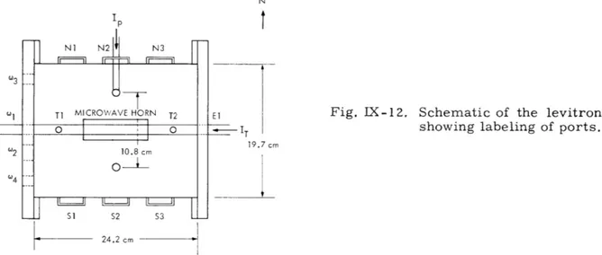
IN A LEVITRON

We shall report on an investigation of the stability of an electron cyclotron resonance heated plasma in a levitron, shown schematically in Fig. IX-12. Heating was accom-plished with a 1-MW, 10-is pulse of microwaves with frequency approximately 2. 8 GHz (S-band). The poloidal magnetic field was produced by discharging a capacitor bank into a circular coil, which entered the chamber through port N2. The toroidal field was cre-ated by discharging a capacitor bank through several turns of wire inside a longitudinal

N

Fig. IX-12, Schematic of the levitron showing labeling of ports.

bar that entered at ports El and W1 and passed perpendicularly through the center

of the coil. The toroidal field affected the shear, or twist, of the magnetic field lines.

Electron-cyclotron heating occurred on a range of surfaces about the 1-kG surface,

which formed a torus around the poloidal magnet. The diagnostics utilized included a

(IX. APPLIED PLASMA RESEARCH)

phototube, single and double probes, and 8 wall-loss probes situated symmetrically in the plane of the poloidal coil, 1. 0 cm off the wall, as shown in Fig. IX-13.

MICROWAVE

HORN

LP2 LP3

LPI POLOIDAL LP4

PORT 52 MAGNET PORT N2 TOROIDAL

MAGNET- POLOIDAL MAGNET

MECHANICAL SUPPORT AND CURRENT LEADS

LP8 LP5

LP7 r-- 18 WIRE LP6

TEFLON TUBING

VACUUM PUMPS

Fig. IX-13. Positioning and labeling of wall-loss probes.

The magnetic configuration of the levitron was proposed by Lehnert, in 1958.1 Levitron experiments, principally at the Lawrence Radiation Laboratory2 and at the Culham Laboratory, have produced plasmas with densities of from 1010 to 1012 cm-3 with electron temperatures of 1-30 eV, and with energy decay times typically of 5-30 times the Bohm time. A similar device, the spherator,4 is in operation at the Plasma Physics Laboratory, Princeton University.

Basic Plasma Properties

a. Microwave Heating

The microwaves were triggered at the peak of the magnetic current. The magnetic field decayed approximately 4% during the lifetime of the plasma. The 10-vs micro-wave pulse ionized and heated the gas in the chamber, typically Hydrogen or Argon at

-5

pressures of ~10-5 Torr. The dispersion relation for electromagnetic waves propa-gating in a plasma in the absence of a magnetic field predicts total reflection of the microwaves when the gas has been ionized to the extent that the electron density is such that the plasma frequency exceeds the microwave frequency. This corresponds to a

10 -3

density of 9 x 10 cm . This dispersion relation was modified by the presence of the magnetic field and by the geometry of the levitron. The reflection phenomena was qual-itatively observed on the reverse microwave power monitor.

b. Nature of the Plasma

The light output of the plasma, which could be observed with the naked eye, was

mea-sured with a phototube. Figure IX-14a shows the phototube output for a Hydrogen plasma

with a neutral-particle pressure of 4. 3 X

10

Torr.

There are three discernible

peaks: at t

=

2, 7, and 12

ps.

Time is measured from the start of the microwave pulse.

Figure IX-14b shows the output for a hydrogen plasma with a neutral-particle pressure

-

(a)

Fig. IX-14.

wave pulse. Horizontal scale:

5 ts/div.

I =

6000 A.

It

=

1000 A.

(a)

Hydrogen, 4.3 X

10

Torr. (b)

Hydrogen,

8.6 X 106 Torr.

(c) Argon, 4. 2 X

10

Torr. (d)

Argon, 8.4 X

10

Torr.

-

(d)

-6

of 8. 6 X

10

Torr, with peaks at t

=

2, 10, and 15

p.s.

The first peak corresponds to

the breakdown of the hydrogen. The later peaks are probably the result of

ionizations

caused by collisions between electrons heated by cyclotron resonance and neutrals.

Fig-ure

IX-14c and IX-14d shows the phototube output for an Argon plasma with

neutral-particle pressures of 4. 2 X

10

and 8.4 X

10

Torr, respectively. The breakdown

peak at

t

=

2

ps

is less prominent than with hydrogen.

The later peaks are at

t

=

9,

14,

and 25

ps.

The plasma density and electron temperature were measured by using standard

elec-trostatic and double floating probe techniques. The density measurements were

cor-rected for electron Debye length effects with the method of Laframboise.5 The electron

temperature of the Hydrogen plasma of neutral-particle pressure of ~4-6 X

10

Torr

was measured to be 30-70 eV at

densities of ~1 X 1010 cm

immediately after the end

(IX. APPLIED PLASMA RESEARCH)

of heating.

At a neutral-particle pressure of ~9 x 10-6 Torr, the electron

ture was 120 eV at densities of 1

X

10

cm

This represents 2% ionization. Argon

plasmas were hotter and denser.

An electron temperature of 100 eV and density of

1 X 1011 cm-

at t

=

20 is were achieved at a neutral-particle pressure of 4X 10 5 Torr.

-6

At a neutral pressure of 8 X 106 Torr, the electron temperature was 135 eV at

11

-3

~1 X 10

cm

Several density profiles were measured. Figure IX-15 shows a density profile

mea-sured from the toroidal magnet out to the inner radius of the poloidal magnet, and from

the outer radius of the poloidal magnet to the wall-loss probes that were grounded to act

as limiters. The longitudinal profile was measured from the surface of the poloidal

1.0 - POLOIDAL MAGNET -0.5 LONGITUDINAL 0 - TOROIDAL MAGNET I 0.6 1.2 1.8 2.4 3.0 cm - LIMITER WALL 1.0 0.5 _{0. RADIAL} 0 1 2 3 4 5 6 7 8 9 10 1 kG 1 kG

Fig. IX-15. Radial and longitudinal density profile.

Hydrogen,

-5

4.3 X 10 Torr. I = 6000 A. I = 1000 A. t = 15

JLs.

magnet outward in a direction perpendicular to the plane of the poloidal magnet.

The

density gradients were observed to be of the order of 1 cm near the poloidal magnet, and

0. 5 cm near the toroidal magnet.

The plasma floating potential was measured with a high input impedance,

wide-bandwidth amplifier. For a Hydrogen plasma with a neutral-particle pressure of 4. 3

X

-5

10

Torr, the floating potential within the poloidal coil typically rose to 15 V positive

at t

=

6-8 Vs as electrons were lost. As the electron loss rate changed, the floating

potential declined to 10-15 V negative at t

=

15

ps,

and then decayed to zero. At the

wall-loss probes, the floating potential typically rose to 8 V positive at t

=

1 Ls, dropped

to 5 V negative at t

=

2 is,

rose to 10 V positive at t

=

6

ps,

and then decayed to zero

with a time constant of 40-60 Vts.

Experimental Observations

a. Asymmetries

Asymmetries were noted in the plasma floating potential and plasma density in the vicinity of the poloidal coil support. The ion saturation current was measured using the wall-loss probes, and found to be isotropic except at the probes just above (LP4) and

-5 below (LP5) the poloidal support. At a neutral-particle pressure of 4. 3 X 10-5 Torr of Hydrogen and at high values of shear, the plasma density was higher above the sup-port and lower below the supsup-port than that measured at the other wall-loss probes. The density ratio of above the support to below the support was 1. 8. At lower values of shear, the density above the support decreased, though it was still above normal, while the density below the support increased to values above normal. The density ratio declined to 1.1. Figure IX-16 shows the ion saturation current as measured at the LP2, LP4, and LP5 wall-loss probes. The floating potential was significantly higher as mea-sured with LP4 than with LP5, as shown in Fig. IX-16b. The potential at LP5 was essen-tially the same as that measured at the probes far from the support. The potential at

LP4 remains at 15 V positive from t = 15 to t = 45 is. This is 5-10 V higher than at LP5. The floating potential at LP3 was similar to that at LP4, thereby indicating that the extent of the potential perturbation was ~10 cm above the support.

Insertion of a Langmuir probe through port S2 was observed to reduce the floating potential by approximately 20% at LP1 and to have no effect on LP8.

The presence of the poloidal support could have caused a density gradient along mag-netic field lines. As the isobaric surfaces would no longer coincide with the magnetic surfaces, an electric field could exist. The E X B drift can result in plasma loss across magnetic field lines. This phenomenon is known as convective cell loss.4' 6-9

b. Oscillations

The levitron plasma was free of large-amplitude oscillations. The normalized amplitude was generally well under 10%, except during microwave heating, when the single-probe measurements oscillated violently. Figure IX-17a shows ion saturation current inside of the poloidal coil. The oscillations during heating were -1 MHz.

Oscillations were observed in the afterglow using the double floating probe. Fig-ure IX-17b and IX-17c shows the probe current for bias voltage of 10 and 30 V,

respec--5

tively, at a neutral pressure of 4. 3 X 10-5 Torr of Hydrogen. The oscillations were 300-500 kHz. Figure IX-17d shows the probe current for a bias voltage of 60 V at a neu-tral pressure of 4. 2 X 10-5 Torr of Argon. The oscillations were 800-1000 kHz. The

double probe was situated within the poloidal ring, 1. 0 cm from the coil surface. These oscillations in the afterglow could not be explained by cyclotron waves. The ion-cyclotron frequencies were typically ~500-2000 kHz for Hydrogen and 10-60 kHz for

.,-

ZERO

(a)

TOP

(a)

CENTER

(a)

BOTTOM

(b) TOP

(b) CENTER

(b)

BOTTOM

Fig. IX-16.

Asymmetries near the poloidal

mag-net support. Neutral pressure: 4. 3

X

-5

10

Torr of Hydrogen.

(a) Ion

satu-ration current

at wall-loss probes.

Horizon-tal scale: 5

ps/div.,

beginning at t

=

10 p.s.

Upper:

LP2 probe.

Middle:

LP4. Lower: LP5.

(b) Plasma

float-ing potential at wall-loss probes. I =

6000 A. It

=

1000 A.

Horizontal scale

is 10 ps/div., beginning at t= 0. Upper:

LP2. Middle: LP4. Lower: LP5.

Fig. IX-17.

Plasma oscillations inside of poloidal

coil.

Horizontal scale is 5

ps/div.

satu-p

t

-5

ration current for 4. 3

X

10

Torr of

Hydrogen.

(b) Double-probe current

for a bias voltage of 10 V for 4. 3

X

-5

10

Torr of Hydrogen. (c) Same as (b)

with bias voltage of 30 V.

(d)

Double-probe current for a bias voltage of

60 V for 4. 2

10-5 Torr of Argon.

60 V for 4. 2 x 10

Torr of Argon.

(a)

(b)

(c)

Argon.

The drift wave frequency was several hundred kHz.

c. Confinement

The plasma confinement was experimentally determined by analyzing the density

decay observed with single and double probes, light emission decay observed with the

phototube, ion saturation current decay observed with the wall-loss probes, and the

Fig. IX-18.

Changes in decay rates.

(a) Ion saturation

current out of the plane of the poloidal coil

for 6.4X10

Torr of Hydrogen. I

=

16000A.

(b)

It

=

4000 A. Horizontal scale is 10

s/div. ,

beginning at t

=

0.

(b) Ion saturation current

inside of poloidal coil for 4. 3 X 105 Torr of

Hydrogen.

I = 8000 A.

I

= 1000 A.

Hor-izontal scale is 5 is/div., beginning at t

=

0.

(c) Double-probe current inside of poloidal

(C)

coil for a bias voltage of 50 V.

I

=

6000 A.

I

= 1000 A.

Horizontal scale is 5 Ls/div.

(d) Ion saturation current at LP4 wall-loss

probe for 8.4 X 10-6 Torr of Argon.

I =

6000 A.

I

= 1000 A.

Horizontal scale is

(d)

5 is/div. (e) Plasma floating potential

out-side of poloidal coil for 4. 3 X 10

Torr of

Hydrogen.

I = 6000 A.

I

= 1000 A.

Hor-izontal scale is 5

ps/div.

Vertical scale is

10 V/div.

(e)

decay of the floating potential. The plasma parameters, particularly the density, slowed

their decay rates by approximately a factor of two soon after the end of microwave

heating, as seen in Fig. IX-18. The plasma was studied during the second density decay

rate and the data are presented in Table IX-1.

The Bohm time of the plasma was given by

(IX. APPLIED PLASMA RESEARCH)

where A is the diffusion length. With a density gradient of -1. 0 cm as the diffusion length, the Bohm time for the Hydrogen plasma at 4. 3 X 10- 5 Torr was approximately 3 [s. For the Argon and lower pressure Hydrogen plasma with higher electron tem-perature, the Bohm time was approximately 1 [is.

Table IX-1. Decay times. I _p = 6000 A. It _t= 1000 A.

Hydrogen Argon

(Torr) (Torr)

Diagnostic 4. 3 X 10 8.6 X i0 4.2 X 10-5 8.4 X 106

(4s)

(is)

(4s)

([s)

Density decay: 45 30 30 30

double floating probe

Density decay: 27 (a)

single probe

Light emission decay: 67 75 70 55

phototube

Ion saturation current decay: 20 (b) 17 48

wall-loss probes

Floating potential decay: 55 55

wall-loss probes

Floating potential decay: 100 (c) single probe Bohm time 3 1 1 1 (a) I = 15,000 A, I = 4000 A, p P t -5 = 6.4 X 10 Torr. (b) I = 12,000 A. P

(c) Situated 1.0 cm from the outer radius of the poloidal coil.

If the sole source of particle loss were due to the interception of particle orbits by the poloidal coil support, the plasma decay time would have been: Ts = nV/2(nAv/4), where nV is the total number of ions, and nAv/4 was the arrival rate of the slower par-ticle, the ions, at velocity v, onto one side of the support of cross-sectional area A. The average ion arrival velocity was given by (8kTe/mi) 1/2. Thus we find Ts = 30 [s

-5

for Hydrogen at 4. 3 X 105 Torr.

In view of the magnitudes of the support loss time and of the ion saturation current decay time at the wall-loss probes, the plasma appears to have been lost during heating and immediately thereafter across magnetic field lines to the walls, but after the break in time constants the plasma loss was mainly to the support.

References 1. B. Lehnert, Nature 181, 331 (1958).

2. 0. _{A. Anderson, D. H. Birdsall, C. W. Hartman, E. J. Lauer, and H. P. Furth,} "Plasma Confinement in the Levitron," in "Proceedings of a Conference on Plasma Physics and Controlled Nuclear Fusion Research at Novosibirsk, U. S. S. R., 1968" (International Atomic Energy Agency, Vienna, 1969), Vol. 1, p. 443.

3. A. F. Kuckes and R. B. Turner, "Plasma Confinement in a Small Aspect Ratio Lev-itron," in "Proceedings of a Conference on Plasma Physics and Controlled Nuclear

Fusion Research at Novosibirsk, U.S.S.R., 1968," op. cit., Vol. 1, p. 427.

4. _{S. Yoshikawa, M. Barrault, W. Harries, D. Meade, R. Palladino, and S. von Goeler,} "Linear Multipole and Spherator Experiments," in "Proceedings of a Conference on Plasma Physics and Controlled Nuclear Fusion Research at Novosibirsk, U. S. S. R.,

1968," op. cit., Vol. 1, p. 403.

5. _{J. G. Laframboise, "Theory of Spherical and Cylindrical Probes in a Collisionless,} Maxwellian Plasma at Rest," UTIAS Report No. 100, University of Toronto Institute

for Aerospace Studies, 1966.

6. R. Freeman, M. Okabayashi, H. Pacher, G. Pacher, and S. Yoshikawa, Phys. Rev. Letters 23, 756 (1969).

7. M. Yoshikawa, T. Ohkawa, A. A. Schupp, Phys. Fluids 12, 1926 (1969).

8. S. Yoshikawa, R. Freeman, and M. Okabayashi, "Effect of Neutral Particles and Supports on the Confinement of Plasma in the Spherator," Report MATT-706, Plasma Physics Laboratory, Princeton University, 1969.

9. _{S. Yoshikawa, "Spherator and Related Experiments," Report MATT-735, Plasma} Physics Laboratory, Princeton University, 1969.

2. QUIESCENT RADIOFREQUENCY PLASMA EXPERIMENT

A steady-state collisionless plasma with a low level of turbulence has been generated in a solenoidal geometry using a Lisitano coil. Electron density varies from 0. 1 to 2. 0 X

11 -3

10 cm , and electron temperature from 3 eV to 10 eV, depending on the radial posi-tion and the coupled RF power. At an operating pressure of 10- 5 Torr both electrons

and ions are collisionless with respect to the neutrals (c T.ien >> 1). For low-frequency

long-wavelength instabilities such as drift waves (small kll), the high density case is near the electron-ion collisional threshold (wdTei i), while for the lower density case the plasma is collisionless ( dTei >> 1). Low-frequency turbulence (0-30 kHz) is peaked

at the plasma edge similarly to edge oscillations found in Q-machines. The amplitude, coherence, and frequency spectrum can be varied to some extent with end-plate biasing. These plasma characteristics are suitable for studying turbulence and transport phenom-ena.

System

A schematic diagram of the system is shown in Fig. IX-19. It is a modified form of the HCD-III which was used by D. J. Rose and J. C. Woo.1 The stainless-steel

(IX. APPLIED PLASMA RESEARCH)

vacuum can (14. 6 cm ID) has been lengthened to 350 cm and two diffusion pumps and

magnets have been added.

The system can now be operated either as a mirror machine

or as a solenoid with magnetic field variable from 0 to 3. 5 kG in any section.

Since the

3.5 m

UNIFORM FIELD 2.0 m I

_ COIL

CONDUCTING SCREEN PUMP

INSULATING END PLATE (NOT DRAWN TO SCALE)

Fig. IX-19.

Schematic of the system.

operation of the Lisitano coil is based on electron-cyclotron resonance heating (ECR)

the regulation of the mirror fields has been improved to 0. 5%.

Neutral pressure is

con-trolled with double baffles of 5-cm aperture, and a third baffle can be installed for

oper-ation with a coil at the other mirror. Neutrals are introduced into the coil region by a

variable flow gas feed and are trapped in the coil region by the baffles.

Coil Design

A schematic diagram of the coil is shown in Fig. IX-20.

The design is similar to

those used by Lisitano.

The coil can be visualized as a slotted microwave antenna

folded onto a conducting metal cylinder so that the electric field across the slot lies in

a plane perpendicular to the coil axis.

A conducting cylindrical shield is placed

concen-trically over the slotted cylinder to prevent outward radial power loss. With the shield

installed, power can radiate only as TE or TM modes inside the slotted cylinder.

By

choosing the radius sufficiently small, these modes are cut off and only an evanescent

field can exist in the coil.

One end of the slot is made one-quarter wavelength long to

isolate the end from the power feed.

The rest of the slot, which is folded onto the coil

and couples energy into the plasma, is made a nonintegral number of half-wavelengths

long to avoid an impedance mismatch where the power is fed into the coil.

RF power at

3 GHz is coupled through the shield to the slot as shown in Fig. IX-20.

For ECR heating,

a 1-kG field in the slot region is necessary.

The 0. 5% regulation of the magnetic field

15.2 cm 2.54 cm

I

(a)

£1111

(NOT DRAWN TO SCALE)

(b)

_(c)

Fig. IX-20. Schematic of the coil.

is sufficient if the coil is operated in a small magnetic field gradient. If the field is too flat, erratic operation is incurred and more regulation is needed.

By constructing the coil with both ends open, magnetic field lines passing through the coil aperture will also pass through the end plates, thereby ensuring good contact between the end plates and the plasma. This was found to be important for turbulence control.

Density is limited by electron shielding of the coil slots. For a resonant magnetic field, this corresponds to the upper hybrid cutoff condition, that is,

2

2

p= N (N+ 1) Oce

p ce'

where N is the harmonic number wRF/ice. For the first harmonic this corresponds to 11 -3

a density of 2. 2 X 10 cm .

An indication of the effect of ECR heating on the electron distribution function can be made by calculating the perpendicular energy gained by an electron making a single pass through the resonance region of the coil. An electron with temperature T at an angle 60 to the magnetic field will undergo heating for an effective correlation time determined by the temperature, the RF source bandwidth, and the field gradient. The heating width of the resonant region can be related to the source bandwidth and field

(IX. APPLIED PLASMA RESEARCH)

gradient as follows:

AfRF

fRF B B

where XB is the magnetic field scale length (B d . It follows that the correlation time is

Ax vll (Oo ,T)

and the change in perpendicular energy of an

Te 0.1

electron for a single transit through the

coil will be (in eV)

eE

AW(T,

0o)=

For the magnetic field, slot width, and

applied power used in our system, a

typ-ical electron will receive the energy change

(in eV)

0

AW vs 0 for various

elec-tron temperatures.

which is plotted in Fig. IX-21.

It follows from Fig. IX-21 that the energy gained is only a few eV for a typ-ical particle, while a small population of electrons receive over 100 eV. Since the ion saturation current collected by a cold spherical probe is several orders of mag-nitude less than electron saturation cur-rent, these hot electrons may introduce errors in floating-potential measurements. For our plasma, this population should be small, since electrons are axially trapped in the plasma column by the sheaths at the end plates. The hottest electrons should scatter in angle off the background neutrals and escape through the end sheaths. All particles will scatter in angle off the neu-trals, but only the very hot electrons can

pass through the sheath potential. Since the ions migrate slowly to the end sheaths, the electrons are contained for a period much longer than the electron-electron thermaliza-tion time. It is concluded that most electrons that are trapped in the column should have a Maxwellian distribution. This was verified with probe characteristic curves. At low density, however, where the thermalization time is long, current collecting probes had to be biased at probe/T - 20 to obtain good results for ion saturation current.

Plasma Properties

A cylindrical plasma column, 350 cm long and 3-4 cm in diameter, was formed by coupling 3-20 W of RF power to the plasma. The gas was Argon at a pressure of 3-7 X

-4

-10-4 Torr in the coil region and 0. 6-1. 5 X 10-5 Torr in the baffled region. For these pressure ranges, the general properties were insensitive to small changes in neutral pressure. By varying the coupled power to the plasma (incident minus reflected power) the density was varied over an order of magnitude as shown in Fig. IX-22.

Spherical probes with a radius of 0. 57 mm were used to measure density and tem-perature. Since the ion Larmor radius is much larger than the probe radius, collision-less probe theory was used.6, 7

A typical density profile is shown in Fig. IX-23 for 12 W of power coupled to the plasma. The radial density profile was found to be insensitive to coupled power and changed only in magnitude. The profile appears to be radially limited by the coil inner radius (1. 25 cm).

Electron temperatures for 12 W and 5 W power yield similar radial profiles (Figs. IX-24 and IX-25); however, more efficient electron-ion thermalization at higher densities results in a lower electron temperature for 12 W. The ion temperature is sen-sitive to the ratio of electron-to-neutral density and is expected to be approximately 0. 4 eV for our experiment.5 It is of interest that electron temperature and density gra-dients are opposed out to a radius of 0. 75 cm; however, coherent oscillations indicating an instability in this region were not observed.

Plasma Turbulence

Broadband low-frequency turbulence and coherent modes have been observed. Broadband low-frequency turbulence (0-30 kHz) appears at all radii but has a max-imum at the plasma edge. On the column axis it is only a few percent as shown in Fig. IX-26, but increases to over 10% near the inner radius of the coil. Beyond a radius of 1. 25 cm, the plasma becomes fully turbulent and probe measurements indicate a "flutelike" motion of the plasma. Figure IX-27a shows the spectrum 0-100 kHz of log (An) and Fig. IX-26 shows the radial dependence. This condition is found at all

2.0 -1.6 1.2 0 2-- 0.8 z 0.4 0 0 2 4 6 8 10 12 14 16 18 20 COUPLED RF POWER (W)

Fig. IX-22.

Electron density vs coupled power.

1.6 1.4 0 12 W B= 1 kG 1.2 ION E ILARMOR S 1.0 - _RADIUS o - 0.8

z

0.6 I COIL EDGE ( GEOMETRIC)

0.4

0.2

0 0.50 1.00 1.50 2.00 RADIUS ( cm)

B= kG

COIL EDGE ( GEOMETRIC)

0.50 1.00 RADIUS ( cm) 1.50 2.00 - 5 W 12 VA B 1 .kG

COIL EDGE ( GEOMETRIC)

Fig. IX-24.

Electron temperature vs radius.

Fig. IX-25.

Floating potential vs radius.

1.50

RADIUS ( cm)

An n 0.16 0.14 0.12 0.10 0.08 0.06 0.04 0 0.50 1.00 RADIUS (cm)

Fig. IX-26.

(a)

COIL EDGE ( GEOMETRIC)

1.50 2.00

An/n vs radius, rms.

(b)

(a)

(b)

(c)

Fig. IX-28. An, 12-2 kHz, rms: (a) +20 V end-plate biasing;

(b) 0 V; (c) -20 V.

operating densities and resembles edge oscillations found in Q-machines.8 Figure IX-28

shows how this spectrum can be controlled by end-plate biasing. The photographs show

the degree of control over An, 2-12 kHz.

It is possible to turn on or off a coherent

mode near 4 kHz by properly biasing the end plates.

Since density and temperature

gra-dients are small and the radial electric field is large near the edge, the turbulence may

be a Rayleigh-Taylor flute or a Kelvin-Helmholtz instability driven by the radial electric

field. The dependence upon end-plate biasing supports the theory that the waves are

driven by the radial electric field. The flutes appear to be m

=

1 modes.

For densities greater than 1011 cm

a coherent wave was observed centered at a

radius of 1. 5 cm.

This also appears in a region where density and temperature

gra-dients are small. Figure IX-27b shows this wave.

J. E. Robinson, E. Oktay, L. M. Lidsky, R. A. Blanken

References

1. J. C. Woo, Sc. D. Thesis, Department of Nuclear Engineering, M. I. T., June 1966.

2.

G. Lisitano, R. A. Ellis, W. M. Hooke, and T. H. Stix, Report MATT-Q-24,

Plasma Physics Laboratory, Princeton University, 1966.

3.

G. Lisitano, private communication (1969).

4.

P. Politzer, private communication (1969).

(IX. APPLIED PLASMA RESEARCH)

5. M. Hudis, K. Chung, and D. J. Rose, J. Appl. Phys. 39, 3297 (1968).

6. J. G. Laframboise, Report 100 University of Toronto, Institute for Aerospace Stud-ies, 1966.

7. F. F. Chen, C. Etievant, and D. Mosher, Phys. Fluids 11, 811 (1968). 8. D. L. Jassby and F. W. Perkins, Phys. Rev. Letters 24, 256 (1970).