Approximation algorithms for stochastic scheduling problems
Texte intégral
Figure
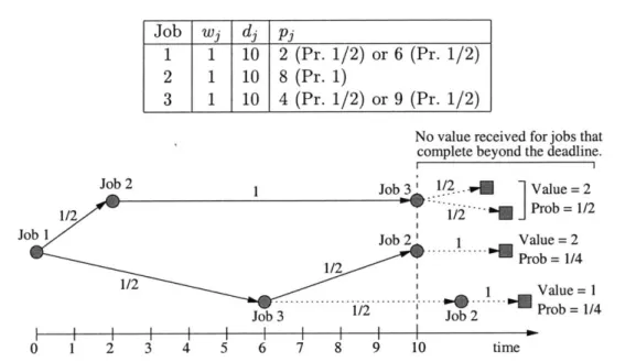
![Figure 1-3: An instance of 1 1 p 3 ~ stoch, dj = d I E[ wjVj] with adaptivity gap 4 - 2'/2 > 1.171](https://thumb-eu.123doks.com/thumbv2/123doknet/14070109.462261/21.918.243.646.391.477/figure-instance-stoch-dj-i-wjvj-adaptivity-gap.webp)

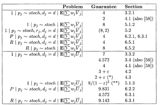

![Figure 4-1: Approximation of the function G(t) GJu{J},k,6/3(t) (shown by a dotted line) by a piecewise constant function f(t) so that f(t) E [G(t)/(1 + 6/3), G(t)].](https://thumb-eu.123doks.com/thumbv2/123doknet/14070109.462261/67.918.213.694.163.376/figure-approximation-function-shown-dotted-piecewise-constant-function.webp)


Documents relatifs
sequence, number of his study employs the production scheduling of crystalline silicon solar cells as a case study that focuses to establish a suitable product planning and
An exponential algorithm solves opti- maly an N P -hard optimization problem with a worst-case time, or space, complexity that can be established and, which is lower than the one of
Using strategies similar to those used in such algorithms, we show how to extend a first-order solver (in this case Kod- kod, a model finder for relational logic used as the engine
Calcium silicate hydrate (C-S-H) was prepared in the presence of aniline monomer followed by in situ polymerization in order to increase the degree of interaction between
(Bouchard, 2007) C’est pourquoi les proches d’une personne mise en maison d’arrêt sont stigmatisés. De plus, comme les trois hommes ont été condamnés à une peine privative
16. Projet de décret portant le Code de la prévention, de l’aide à la jeunesse et de la protection de la jeunesse, exposé des motifs, Doc., Parl.. aux enfants et à leur
A batch siz- ing and scheduling problem on parallel machines with different speeds, maintenance operations, setup times and energy costs.. International Conference on
There are two possible measures for the impact caused by the schedule changes [19]: (1) the deviation from the original jobs starting times, (2) the deviation from the
