Non-invasive multilevel geometric regularization of mesh-based 3D shape measurement

HAL Id: hal-02431948

https://hal.archives-ouvertes.fr/hal-02431948

HAL is a multi-disciplinary open access archive for the deposit and dissemination of sci-entific research documents, whether they are pub-lished or not. The documents may come from teaching and research institutions in France or abroad, or from public or private research centers.

L’archive ouverte pluridisciplinaire HAL, est destinée au dépôt et à la diffusion de documents scientifiques de niveau recherche, publiés ou non, émanant des établissements d’enseignement et de recherche français ou étrangers, des laboratoires publics ou privés.

Non-invasive multilevel geometric regularization of

mesh-based 3D shape measurement

Guillaume Colantonio, Morgane Chapelier, Robin Bouclier, Jean-Charles

Passieux, Eduard Marenic

To cite this version:

Guillaume Colantonio, Morgane Chapelier, Robin Bouclier, Jean-Charles Passieux, Eduard Marenic. Non-invasive multilevel geometric regularization of mesh-based 3D shape measurement. Inter-national Journal for Numerical Methods in Engineering, Wiley, 2020, 121 (9), pp.1877-1897. �10.1002/nme.6291�. �hal-02431948�

DOI: 10.1002/nme.6291

ARTICLE TYPE

Non-invasive multilevel geometric regularization of mesh-based

3D shape measurement

Guillaume Colantonio

_{| Morgane Chapelier}

_{| Robin Bouclier}

_{| Jean-Charles Passieux*}

_{| Eduard}

Marenić

1_{Institut Clement Ader (ICA), Université de}

Toulouse, CNRS-INSA-UPS-ISAE-Mines Albi, Toulouse, France

2_{Institut de Mathématiques de Toulouse}

(IMT), Université de Toulouse, CNRS-INSA-UT1-UT2-UP, Toulouse, France Correspondence *J.C. Passieux Email: passieux@insa-toulouse.fr Present Address

135 avenue de Rangueil, 31077 Toulouse, Fr.

Summary

Finite element stereo digital image correlation (FE-SDIC) requires a crucial calibra-tion phase in which the initial CAD needs to be updated to fit the actual shape of the specimen. On the one hand, the use of a FE mesh facilitates the coupling of measure-ments with simulation tools. On the other hand, it provides a unique, fine description of both the geometry and the displacement, which often makes the shape measure-ment problem highly ill-posed. As a remedy, we propose a hybrid isogeometric-FE strategy that can measure a shape in terms of spline functions while considering as an input and output the analysis-suitable FE mesh. Making use of the appealing spline refinement procedures and of Bézier-based operators, multilevel smooth spline dis-cretizations are built concurrently with the initial FE subspace and related to the multi-scale images used for the initialization of the shape measurement. It results in a geometrically sound regularization which provides a spline parametrization of the optimal shape along with its FE twin. A non-invasive implementation from an existing FE-SDIC code is also detailed. The performance of the proposed method is assessed on real images and comparisons are made with other published techniques to prove its efficiency.

KEYWORDS:

Stereo-correlation, Finite elements, Free-form surfaces, NURBS, Multilevel design, Bézier extraction

1

INTRODUCTION

The expanding use of finite elements (FE) meshes in digital image correlation (DIC) algorithms1,2,3,4,5,6,7,8,9,10 _{is explained by} their ability to be coupled with numerical models. The interaction of measurement and simulation becomes fast and friendly, as both kinematic fields are defined at the nodes of the same mesh. This potent framework paves the way to a better integration of models and experiments in solid mechanics11,12,13,14,15.

When the specimen geometry or mechanical loading is not planar, a stereo digital image correlation (SDIC) method is used concurrently with, at least, two cameras, to access the three components of the displacement at the surface of the specimen. This method, initially developed in the context of subset-DIC16,17_{, was recently extended to the context of global approaches}11,18,13_. For instance, global SDIC was successfully used for the analysis of complex experiments such as structural tests19,14,20. Before estimating the displacement measurement, SDIC requires a calibration phase aiming at determining the parameters of the cam-eras and the actual shape of the specimen. In FE simulations (and thus in FE-SDIC), a unique interpolation subspace is generally

used for both the approximation of the geometry and of the displacement (basic principle of isoparametric finite elements). The approximation subspace is therefore entirely defined by the choice of a FE mesh.

However, the shape of the specimen is generally rather smooth and regular and it should require less degrees of freedom than the displacement field which may comprise important gradients. Another way of considering FE-SDIC would consist in a suitable mix of an appropriate mesh for shape measurement and a different finer FE mesh that properly compute the displacement (i.e., an analysis-suitable mesh). Using standard finite elements, such an approach would require non-trivial projection procedures between unstructured 3D surface meshes, which are often accompanied with a modification of the (generally curved) geometry. To resolve this issue, the common practice consists in using a refined analysis-suitable FE mesh for both shape and displace-ment measuredisplace-ments, which could make the shape measuredisplace-ment problem highly ill-posed. As a result, regularization techniques based on the addition of specific terms19,13_{are often used to avoid getting wiggly, irregular shapes. Such regularization is also} employed in a multi-scale initialization phase which consists in decreasingly filtering the images and modifying the size of the apparent approximation subspace by acting on the regularization level (i.e., modifying the weight of the additional regularizing terms).

From a mathematical and a numerical point of view, we notice that the mesh-based shape measurement problem coming from the experimental mechanics community shares many similarities with the shape optimization problem encountered in structural design. Indeed, structural shape optimization also aims at finding the optimal geometry of a structure and involves a FE mesh in the process21,22_{. The difference only lies in the desired objective which is related to the fulfillment of a certain structural behavior} in shape optimization while it concerns the fitting with the real surface in shape measurement. Therefore, the purpose of this work is to draw inspiration from the techniques developed in the area of shape optimization to improve the field of mesh-based shape measurement.

One approach in shape optimization is actually very close to what is performed for shape measurement: it consists in using the spatial location of the FE nodes as the design variables in combination with delicate mesh regularization techniques to prevent the appearance of irregular, "unrealistic" shapes23,24_{. Meanwhile, another class of techniques, denoted by the} computer-aided-design (CAD)-based approach, has also emerged for shape optimization: the idea is to resort to the same spline-based functions as in CAD software to describe the geometry25,26,27_{. The design variables are this time the spatial location of the control points} of the spline entities, which enables to get a light and smooth parametrization of the geometry and of its update28,29_{. The} difficulty in this second family of methods is then transferred to the connection of the (spline-based) geometric and (FE-based) analysis models30,31_{. To answer this issue, one way to naturally proceed is to use the isogeometric analysis (IGA) framework}32,33 which enables to discretize the structure with its intrinsic, spline-based, CAD geometric definition. Isogeometric (IG) shape optimization has thus been successfully applied to a wide range of applications (see34,35,36,37,38_{among others). More precisely, it} is based on a multilevel design concept offered by the spline technology in which one can refine the geometry without altering its initial shape and regularity39_{. As a consequence, different refinement levels of the same spline-based geometry are considered} to define both design and analysis spaces. The coarser level is dedicated to the parametrization of the shape to get "realistic" structures while the finer level defines the analysis model and is set to ensure good quality of the mechanical solution.

A first attempt in applying IGA to shape measurement has been recently performed in Dufour et al.40,18,19_{. In these pioneering} works, the authors considered a higher-order B-spline (monolevel) parametrization of the surface (thereby acting on a geomet-rical object which is consistent with CAD) both for shape and displacement measurements. The authors also went towards the identification of mechanical models by comparing the measured IG displacement field with a computed one using a dedicated IG code12_{. However, besides the effort to implement spline functions in the SDIC framework, the problem is that the user ends} up with an experimental displacement field that is expressed on a spline basis, whereas most simulation tools are based on finite elements. Splines clearly provide flexibility for shape and displacement measurements but make connection with most of today’s numerical models more complex, which is the key advantage of global approaches in DIC.

In this paper, we build a hybrid IG-FE methodology for mesh-based shape measurement that draws up the best of each tech-nology. On the one hand, we consider as an input and output the FE mesh that is fine enough to properly describe the underlying mechanics. In a second step, the FE mesh will thus be suitable for displacement measurement using stereo-correlation and this resulting kinematic field will be easily compared to a computed one obtained from existing, standard FE codes. On the other hand, we undertake to use the splines along with the IG multilevel design concept (performed in shape optimization) for the description of the geometry and of its update in the shape measurement process. The idea here is to couple the multilevel opti-mization process with the multi-scale initialization of shape measurement to get different approximation spaces which naturally follow, at each level, the resolution of the image. The regularization level is thus given by the refinement of the spline spaces which is chosen in accordance with the coarsening of the images (no more need of additional regularization terms). Since it is

based on functions coming from the geometric design community, the proposed regularization scheme has a strong geometrical meaning, that is why we refer to geometric regularization to characterize the technique.

The additional ingredient of our approach is to make use of a recently developed global bridge between IGA and FE analysis (FEA)41 _{to be able to communicate between the different approximation subspaces for the geometry (multilevel spline-based} parametrizations) and for the displacement (analysis-suitable FE mesh). Based on the original idea behind Bézier extraction42 and on more recent Lagrange extraction43_{, this global transformation goes from Lagrange polynomials to (possibly rational)} spline basis, thus enabling to recover an IG operator without implementing IGA but simply by projecting an FE operator onto the reduced, more regular, IG basis. As a result, besides its attractive regularizing features, the implementation of the proposed strategy is non-invasive with respect to FE-SDIC.

The paper is organized as follows: after this introduction, Section 2 specifies the calibration phase occurring in FE-SDIC with a particular emphasis on the shape measurement problem. Then, Section 3 is devoted to the development of the proposed geometric regularization scheme while Section 4 assesses the performance of the methodology through the analysis of several real images and comparisons with other published techniques. This brings us to Section 5 where concluding remarks are drawn.

2

MESH-BASED SHAPE MEASUREMENT

Let us assume that we have an existing description (say a CAD model) of the nominal geometry of the specimen, which, in experimental mechanics, is generally the case. Let Ω𝑠be a surface domain referred to as Region of Interest (ROI) and such that Ω_𝑠⊂ℝ3_{corresponds to the visible surface of the theoretical shape. This representation does not correspond exactly to the} actual shape of the specimen, because of surface roughness, manufacturing defects, pre-load or relaxation of residual stresses, to name a few. In SDIC, the estimation of the real surface is of the utmost importance because it is an essential prerequisite for 3D surface displacement measurement. It may also be used to update the model geometry in validation and/or identification procedures, since kinematic fields may significantly depend on it.

2.1

Camera model

As classically done in SDIC44_{, each camera 𝑐 is equipped with a camera model 𝐏}

𝑐 that maps any 3D point 𝐗 ∈ Ω𝑠expressed in the world reference system_𝑤to the corresponding coordinates in pixels 𝐱_𝑐 in the image frame and is written as:

𝐏_𝑐 ∶ ℝ3→ ℝ2, 𝐗 → 𝐱𝑐= 𝐏𝑐(𝐗, 𝐩𝑐), ∀𝐗 ∈ Ω𝑠, (1)

where 𝐩_𝑐is a vector collecting the model’s parameters. More precisely, camera models 𝐏_𝑐can be either linear (in homogeneous coordinates) or non-linear to take into account lens distortions. It depends on two sets of parameters: the intrinsic parameters (focal length, image center, horizontal/vertical aspect ratio, skew and possible distortion parameters) and the extrinsic parameters (3 rotations and 3 translations that map the reference frame of the specimen_𝑤to that of the imaging sensor_𝑐). The calibration of these parameters must be done prior to any measurement. In this study, intrinsic parameters are calibrated using calibration targets and a classic photogrammetric technique as described in45,46_{. In the remainder of this article, the instrinic parameters will} be assumed to be known and only the extrinsic parameters will be considered, such that for each camera 𝑐, the camera model

𝐏_𝑐 will be entirely defined by 𝐩_𝑐 ∈ ℝ6_.

2.2

Coupled calibration and shape measurement problem

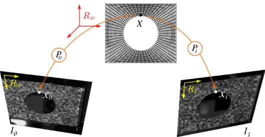
As depicted in Figure 1, the graylevel conservation assumption47 _{supposes that the graylevel value𝑐(𝐱}

𝑐) of the projections 𝐱𝑐 in each image𝑐of any 3D point 𝐗 should be equal:0(𝐱₀) =1(𝐱₁). Since both the actual shape and position of the specimen (with respect to the stereo rig) are not known exactly, the graylevel conservation is not fulfilled. The calibration of the stereo rig thus consists in a coupled problem aiming at finding the extrinsic parameters 𝐩 = [𝐩₀,𝐩₁] in addition to a shape correction field

𝐒(𝐗), ∀𝐗 ∈ Ω𝑠, such that the advection of the nominal surface Ω𝑠by the correction field 𝐒(𝐗) corresponds to the actual surface. More precisely, shape correction and camera parameters minimize the graylevel mismatch:

𝐒⋆_,𝐩⋆_{= arg min} 𝐒∈𝐿2(Ω𝑠),𝐩∈ℝ12 𝑗(𝐒(𝐗), 𝐩) with 𝑗(𝐒(𝐗), 𝐩) = 1 2∫ Ω𝑆 ( 𝑟(𝐒(𝐗), 𝐩)) 2 d𝐗, (2)

FIGURE 1 Principle of the formulation of the SDIC problem in the reference frame of the FE model. A 3D point 𝐗 and its

projections 𝐱₀and 𝐱₁onto the image planes.

and where the graylevel residual 𝑟(𝐒(𝐗), 𝐩) is defined ∀𝐗 ∈ Ω_𝑠as:

𝑟(𝐒(𝐗), 𝐩)=0 (

𝐏₀(𝐗 + 𝐒(𝐗), 𝐩₀))−1 (

𝐏₁(𝐗 + 𝐒(𝐗), 𝐩₁)). (3)

Let us highlight, at this stage, that the graylevel residual is defined in Ω_𝑠in the reference system of the model which differs from subset based SDIC, where it is written in the image frames.

The unknown vector 𝐩 gathering the extrinsic parameters is already discrete, but the shape correction field 𝐒 lies in an infinite space. To solve Problem (2) an approximation subspace for 𝐒 must be defined. To be consistent with the description of the geometry and displacements in FE simulations, 𝐒 is searched for in an analysis-suitable FE subspace13_:

𝐒(𝐗) = 𝑛𝐹 𝐸 ∑ 𝐼=1 𝐿_𝐼(𝐗) 𝐪𝐼 = 𝐋 𝑇 (𝐗) 𝐪, (4)

where 𝐋 is a (3𝑛_{𝐹 𝐸} × 3) matrix gathering the 𝑛𝐹 𝐸 Lagrange shape functions 𝐿𝐼 and 𝐪 is a vector that collects the 3𝑛𝐹 𝐸 corresponding degrees of freedom (DOF):

𝐋= ⎡ ⎢ ⎢ ⎢ ⎢ ⎢ ⎢ ⎢ ⎢ ⎢ ⎢ ⎢ ⎢ ⎣ 𝐿₁ 0 0 ⋮ ⋮ ⋮ 𝐿_𝑛 𝐹 𝐸 0 0 0 𝐿₁ 0 ⋮ ⋮ ⋮ 0 𝐿𝑛𝐹 𝐸 0 0 0 𝐿₁ ⋮ ⋮ ⋮ 0 0 𝐿_𝑛 𝐹 𝐸 ⎤ ⎥ ⎥ ⎥ ⎥ ⎥ ⎥ ⎥ ⎥ ⎥ ⎥ ⎥ ⎥ ⎦ and 𝐪= ⎡ ⎢ ⎢ ⎢ ⎢ ⎢ ⎢ ⎢ ⎢ ⎢ ⎢ ⎢ ⎢ ⎢ ⎣ 𝑞₁1 ⋮ 𝑞1_𝑛 𝐹 𝐸 𝑞₁2 ⋮ 𝑞2_𝑛 𝐹 𝐸 𝑞3 1 ⋮ 𝑞3 𝑛𝐹 𝐸 ⎤ ⎥ ⎥ ⎥ ⎥ ⎥ ⎥ ⎥ ⎥ ⎥ ⎥ ⎥ ⎥ ⎥ ⎦ , (5)

In addition, note that 𝐪_𝐼in (4) is the subset of 𝐪 gathering the three components {𝑞_𝐼1, 𝑞_𝐼2, 𝑞_𝐼3} of the field 𝐒(𝐗) associated to shape function 𝐿_𝐼. Problem (2) is a non-linear least-square problem. Its resolution is based on a fixed point algorithm which consists in alternatively minimizing the graylevel functional 𝑗 with respect to 𝐩 (calibration) and to 𝐪 (shape measurement). Herein, it may be mentioned that the alternating iterations are run until the stagnation of (𝐩, 𝐪) is reached, whereas in the literature, only one iteration of the alternating minimization is usually performed. As will be seen in section 4, several iterations between the two minimization problems where necessary to properly measure a real shape far from the initial CAD.

Minimization with respect to camera parameters. The shape correction field 𝐒(𝐗) being fixed, the set of parameters 𝐩 is

the solution of the calibration problem:

𝐩⋆= arg min

𝐩∈ℝ12

𝑗(𝐒(𝐗), 𝐩) (6)

Such a non-linear least-square problem is solved using Gauss-Newton48_{iterations until the stagnation of 𝐩, see}13_{for details.}

Minimization with respect to shape correction field. The extrinsic camera parameters 𝐩 being fixed, the DOF vector 𝐪 is

the solution of the shape measurement problem:

𝐪⋆= arg min

𝐪∈ℝ3𝑛𝐹 𝐸

𝑗(𝐋𝑇(𝐗) 𝐪, 𝐩) (7)

This non-linear least-square problem is also solved using a Gauss-Newton algorithm. At iteration 𝑘, the solution is sought as

𝐪𝑘_{= 𝐪}𝑘−1_{+ 𝐝}𝑘

𝑞, where the descent direction 𝐝 𝑘

𝑞is the solution of the following linear system 13_: 𝐇𝑘_{𝐹 𝐸}𝐝𝑘_𝑞= 𝐛𝑘_{𝐹 𝐸} with ⎧ ⎪ ⎪ ⎨ ⎪ ⎪ ⎩ 𝐇𝑘 𝐹 𝐸 = _∫ Ω𝑠 𝐋(𝐉𝑘 0 𝑇 ∇𝑘 0 − 𝐉 𝑘 1 𝑇 ∇𝑘 1) (𝐉 𝑘 0 𝑇 ∇𝑘 0− 𝐉 𝑘 1 𝑇 ∇𝑘 1) 𝑇_𝐋𝑇 _d𝐗 𝐛𝑘 𝐹 𝐸 = −_∫ Ω𝑠 𝐋(𝐉𝑘₀𝑇∇0𝑘− 𝐉 𝑘 1 𝑇 ∇1𝑘) 𝑟(𝐋 𝑇 _𝐪𝑘−1_{,𝐩) d𝐗} , (8) ∇𝑘

𝑐 = ∇𝑐(𝐏𝑐(𝐗 + 𝐋𝑇𝐪𝑘−1)) with ∇𝑐defining the gradient of the graylevel image𝑐and 𝐉𝑘𝑐 = 𝐉𝑐(𝐗 + 𝐋𝑇𝐪𝑘−1) with 𝐉𝑐being the Jacobian of Projector 𝐏_𝑐 with respect to 𝐗, i.e. such that 𝐉_𝐜𝑖𝑗 = 𝜕𝐏_𝐜𝑖∕𝜕𝑋𝑗. The so-called DIC operator 𝐇𝑘𝐹 𝐸is actually an approximation of the Hessian of 𝑗 (using first-order derivatives only) and −𝐛𝑘_{𝐹 𝐸}corresponds to its gradient with respect to 𝐪. To evaluate the integrals numerically, and since the quantities being integrated are not regular, a classical quadrature technique based on Riemann sums is used with approximately one integration point per pixel, see49,13. The Gauss-Newton loop is run until the stagnation of 𝐪 is reached.

Remark 1. Up to now, the shape correction field was defined as homogeneous to a displacement field, with one component along each three dimension of space. But since a shape correction field tangent to the surface does not actually modify the geometry, Problem (8) is solved in projection onto the normal of the nominal surface. The shape correction field becomes a scalar field. The operator and right-hand side become 𝐙𝑇_𝐇𝑘

𝐹 𝐸𝐙 and 𝐙

𝑇_𝐛𝑘

𝐹 𝐸respectively, with 𝐙 being a 3𝑛𝐹 𝐸× 𝑛𝐹 𝐸operator representing the normal.

Remark 2. During an experiment, change in illumination may occur, which may change locally the gray level values of images. In DIC which is based on a comparison of gray level values, such modulations are taken into account by an affine correction in gray levels12_:

̃

𝑟(𝐒, 𝐩) = 𝛼 𝑟(𝐒, 𝐩) + 𝛽, (9)

where 𝛼 and 𝛽 are adjusted to account for contrast and brightness modulations respectively. These values, usually taken constant in DIC, have to be considered as additional unknowns of the DIC problem. Shape and calibration rely on a measure of the discrepancy between gray levels of images taken by different cameras from different view angles. The issue of brightness and contrast modulation is much more acute. Choosing 𝛼 and 𝛽 as constants may be insufficient. In12_{, 𝛼 and 𝛽 are sought as low} order polynomials, but specular reflections may not be well described by low frequency corrections. In this paper, inspired from subset DIC methods, an elementary brightness and contrast adjustment is performed, considering 𝛼 and 𝛽 as piecewise constants. Images0and1are modified at each iteration such that their average is zero and their standard deviation is one, on each finite element.

Remark 3. As any Newton type algorithm, the question of the initial guess of 𝐩 and 𝐪 is crucial. On the one hand, as stated above, the theoretical shape is supposed to be a good approximation of the actual shape in experimental mechanics, therefore 𝐪 = 𝟎 is a good initialization. On the other hand, the extrinsic parameters are not known. It is usually initialized by picking manually some (at least 3) points on the mesh and on each image. However, even under these conditions, and particularly when the discrepancy between theoretical and real shape is significant, a pyramidal multi-scale initialization technique may be relevant to improve convergence. In FE-SDIC, the idea consists in filtering images and regularizing the shape simultaneously. Instead of filtering images, pixel aggregation (to generate low-definition images) is probably the best idea because of computational speedup. More precisely, starting with coarse images and a high level of regularization, the process consists in decreasingly filtering the images while reducing the regularization level at each considered scale to reach the fine images. A classic way of regularizing is to

resort to Tikhonov regularization technique, i.e. to complement system (8) as follows: (𝐇𝑘 𝐹 𝐸+ 𝜆 𝐀) 𝐝 𝑘 𝑞 = 𝐛 𝑘 𝐹 𝐸− 𝜆 𝐀 𝐪 𝑘−1_{, (10)}

where 𝐀 is a linear operator such that 𝐀 𝐪 expresses the gradient of 𝐒(𝐗) and 𝜆 is a penalization parameter whose value can be interpreted as the filter cutoff frequency (see, e.g.,19,13_{for more details). The larger 𝜆, the higher the regularization level.}

3

GEOMETRIC REGULARIZATION BASED ON BÉZIER EXTRACTION

We now propose to geometrically regularize the FE mesh-based shape measurement problem (7) by projecting it onto more regular spline-based subspaces. We notice that spline functions have already been successfully used in DIC given their high degree of regularity (see, e.g.,50,51,52,53,54). In the context of shape measurement, their interest is expected to be even more important since these functions are particularly adapted to optimize free-form surfaces36,37_.

3.1

Splines: basics and shape modification

The spline technology which has become a standard over the years for geometric modelling in CAD and computer graphics relies on the use of non-uniform rational B-spline (NURBS) functions25,26,27_{. Only the fundamentals are given in the following. For} further details, the interested reader is referred to the references cited therein. The NURBS functions lend themselves to an exact representation of many shapes used in engineering, such as conical sections (circle, ellipse, etc). NURBS are a generalization of B-splines: they can be viewed as rational projections of B-splines. Therefore, they possess many of the properties of B-splines, the most interesting one being their increased smoothness, thus implying few degrees of freedom.

A general expression for a NURBS geometry with parameter 𝝃 ∈ ℝ𝑑_{(𝑑 being the dimension of the space) is written as:} 𝑺(𝝃) = 𝑛𝐼 𝐺 ∑ 𝐼=1 𝑅_𝐼(𝝃)𝐱𝐼 = 𝐑 𝑇 (𝝃)𝐱, (11)

where 𝐑 and 𝐱 denote the matrix of the 𝑛_{𝐼 𝐺}NURBS basis functions and the vector collecting the location of the associated control points, respectively. Note that the same convention as in (4) is used here for the notation. The multivariate NURBS basis functions are obtained from the multivariate B-spline functions 𝑁_𝐼as follows:

𝑅𝐼(𝝃) = 𝑤𝐼𝑁𝐼(𝝃) 𝑊(𝝃) with 𝑊(𝝃) = 𝑛𝐼 𝐺 ∑ 𝑘=1 𝑤𝑘𝑁𝑘(𝝃), (12) and where 𝑤𝐼 denotes the weight of the 𝐼thcontrol point. Given Eq. (12) (and verifying that the B-spline functions satisfy the partition of unity), it may be noticed that if all weights are equal, the NURBS entity turns out to be a B-spline entity. Then, all one needs to do in order to define the multivariate B-spline function 𝑁𝐼at control point 𝐱𝐼is to perform the tensor product of the univariate B-spline functions associated with this point in the different spatial directions. Finally, the 𝑛_{𝐼 𝐺}

11D B-spline basis functions are piecewise polynomials defined by their polynomial degree 𝑝 and a set of non-decreasing parametric coordinates

𝜉𝑖∈ ℝ collected into a knot-vector Ξ = {

𝜉₁, 𝜉₂, .., 𝜉𝑛_{𝐼 𝐺1}+𝑝+1 }

. From knot-vector Ξ, the B-spline basis functions are constructed recursively using the Cox-de Boor recursion formula (see Cohen et al.25_{). The coordinates 𝜉}

𝑖, referred to as knots, divide the parametric space into elements, and the interval[𝜉₁, 𝜉𝑛_{𝐼 𝐺1}+𝑝+1

]

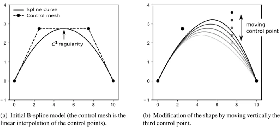
constitutes the patch. Unlike standard FE where each element has its own parametrization, the parametric space of B-spline functions is localized onto the patch, that may be thought of as a macro-element. Several patches can be assembled (similar procedures as for FE assembly) to model complex geometries. As illustrations, Figures 2(a) and 3(a) show two quadratic B-spline curves. These ones result from a linear combination of the univariate B-spline functions depicted at the bottom of Fig. 3(a) using, as coefficients, the control points marked with black circles on each figure. Degree 𝑝 = 2 and knot-vector Ξ ={0, 0, 0, 0.5, 1, 1, 1} are considered for the construction of the B-spline functions.

An interesting feature of splines is their high degree of regularity. If 𝑚 is the multiplicity of a given knot, the functions are

𝐶𝑝−𝑚_{continuous at that location, which is in contrast with standard FE where only a 𝐶}0_{regularity is encountered on the element} boundaries. This property is very appealing from the design point of view since it allows to define smooth free-form shapes using few degrees of freedom. Returning to Figs 2(a) and 3(a), it means that the regularity of the curve between the two elements

regularity Spline curve Control mesh

1

C

(a) Initial B-spline model (the control mesh is the linear interpolation of the control points).

0 2 4 6 8 10 − 1 0 1 2 3 4 moving control point

(b) Modification of the shape by moving vertically the third control point.

FIGURE 2 Spline generation and shape modification: example of a two-element quadratic 𝐶1_{B-spline curve.}

is 𝐶1_{. To modify the shape of the spline entities, one may thus simply need to move the control points, which results in a natural} smooth modification of the geometry (see Fig 2(b) for illustration).

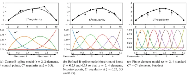
Furthermore, spline functions present refinement procedures which allow to enhance the design space (used for updating the shape) without changing the geometry. In particular, one may refine the spline mesh by inserting knots (knot-insertion technique) while maintaining the initial smooth shape (see Fig 3(b) for illustration). As a result, starting with a coarse spline model, the refinement of the design space can be chosen in accordance with the desired complexity of the final shape. Even more importantly, the modification of the shape can be performed using a multilevel strategy as in IG shape optimization34,36_: one may begin with a coarse design model to fit the major tendencies of the surface and then refine the spline model to get the sharper variations. Eventually, note that matrix representations of the spline refinement procedures are possible; that is, denoting by 𝐑𝑐 _{and 𝐑}𝑓 _{the matrices collecting, respectively, the 𝑛}𝑐

𝐼 𝐺coarse and 𝑛 𝑓

𝐼 𝐺fine spline functions, we can build the refinement operator 𝐂𝑐,𝑓𝑟 such that:

𝐑𝑐_{= 𝐂}𝑐,𝑓 𝑟 𝐑 𝑓 _(𝑛𝑐 𝐼 𝐺≤ 𝑛 𝑓 𝐼 𝐺). (13)

Such a relation offers a simple way to build the refined spline mesh from the coarse one. Denoting by 𝐱𝑐_{and 𝐱}𝑓 _{the location of} the control points associated to the coarse and fine description, respectively, and asserting that the geometry (see Eq. (11)) is not modified through the refinement, we can write the following equality:

(𝐑𝑐(𝝃))𝑇𝐱𝑐 =(𝐑𝑓(𝝃))𝑇(𝐂𝑐,𝑓_𝑟 )𝑇𝐱𝑐, ∀𝝃 ; (14)

which simply leads to:

𝐱𝑓 =(𝐂𝑐,𝑓_𝑟 )𝑇𝐱𝑐. (15)

For more details on refinement strategies of splines and their matrix representations, reference is made to26,39,55_.

Remark 4. NURBS also offer the opportunity to apply shape variation by modifying the control point weights. Nevertheless, unless a very coarse NURBS model is considered56,35_{, it appears from the IG shape optimization community that it is generally} sufficient for free-form surfaces to only use the control point coordinates (see, e.g., Kiendl et al.36_{). We perform similarly in this} work.

Remark 5. In a general context, additional attention may be required when updating the shape for a rather fine spline geometric model. Indeed, if the control points are allowed to independently move in every spatial direction, fold-overs may appear. How-ever, as noted in remark 1, only the normal component of the displacement is considered for the update of the geometry in this study, which naturally circumvents the problem.

3.2

IG-FE bridge

Recalling that the desired input and output in our methodology is the fine (analysis-suitable) FE mesh, it is now required to establish a link between this FE mesh and the different (multilevel) spline-based descriptions introduced in previous section.

Element 1 Element 2 regularity

C1

Nc

(a) Coarse B-spline model (𝑝 = 2, 2 elements, 4 control points, 𝐶1_{regularity at 𝜉 = 0.5).}

regularity

C1

Elements 1 2 3 4

Nf

(b) Refined B-spline model (insertion of knots 𝜉= 0.25 and 0.75 so that: 𝑝 = 2, 4 elements, 6 control points, 𝐶1_{regularity at 𝜉 = 0.25, 0.5}

and 0.75).

Elements 1 2 3 4 regularity

C0

L

(c) Finite element model (𝑝 = 2, 4 standard 𝐶0_{− 𝐶}0_{elements, 9 nodes)}

FIGURE 3 Going from a coarse spline representation to a fine (analysis-suitable) FE mesh without modifying the initial

geometry.

3.2.1

Principle

The ultimate objective is to be able to build, in an explicit and non-invasive manner, the different Hessian and gradient operators, associated to the different spline approximation subspaces, from their fine FE counterparts computed using our FE-SDIC code (see Eqs. (8)). Since it is already possible to communicate between the different spline models (see Eqs. (13) and (15)), the goal here is to relate a fine FE and a fine spline discretization (i.e., with same number of elements and same polynomial degree). In order to do so, we make use of previous work41 _{in which a global algebraic bridge between IGA and FEA is constructed by} resorting to Bézier-based operators42,43_{. More precisely, an operator that maps a 𝐶}0_{FE basis onto a smooth spline basis can be} formulated. Details regarding the construction of this operator are given in forthcoming sections 3.2.2 and 3.2.3.

Considering that we have such an operator in hand and denoting it by 𝐂_{𝐹 𝐸}, we can write:

𝐑𝑓 = 𝐂𝐹 𝐸𝐋, (16)

(𝐋 being the standard nodal Lagrange basis functions of Eq. (4)). As a result, following a similar procedure as in Eq. (14), we can build a FE mesh that fits with the spline geometric model by taking the location of the FE nodes 𝐱𝐹 𝐸_{as follows:}

𝐱𝐹 𝐸= 𝐂𝑇_{𝐹 𝐸}𝐱𝑓. (17)

As an example, this treatment has been performed to obtain the FE model of Fig. 3(c) starting with the spline model of Fig. 3(b). From the resulting FE mesh, we then have the opportunity to recover the refined spline Hessian and gradient operators without implementing IGA but simply by projecting the related FE operators onto the reduced, spline basis. Indeed, from Eq. (8), we can compute the associated spline operator 𝐇𝑓_{𝐼 𝐺}such that (superscript 𝑘 omitted):

𝐇𝑓_{𝐼 𝐺} = ∫ Ω𝑠 𝐑𝑓(𝐉0𝑇∇0− 𝐉1𝑇∇1) (𝐉0𝑇∇0− 𝐉1𝑇∇1)𝑇𝐑𝑓 𝑇 d𝐗 = ∫ Ω𝑠 𝐂_{𝐹 𝐸}𝐋(𝐉₀𝑇∇0− 𝐉1 𝑇 ∇1) (𝐉0 𝑇 ∇0− 𝐉1 𝑇 ∇1) 𝑇_𝐋𝑇_𝐂𝑇 𝐹 𝐸d𝐗 (18) = 𝐂_{𝐹 𝐸}𝐇_{𝐹 𝐸}𝐂𝑇 𝐹 𝐸.

As well, the spline gradient operator 𝐛𝑓_{𝐼 𝐺}can be obtained from its FE counterpart 𝐛𝐹 𝐸(see Eq. (8)) as follows:

𝐛𝑓_{𝐼 𝐺}= 𝐂_{𝐹 𝐸}𝐛_{𝐹 𝐸}. (19)

Furthermore, the same procedure can be applied to recover the coarse spline operators from the fine FE ones: { 𝐇𝑐_{𝐼 𝐺}= 𝐂𝑐,𝑓_𝑟 𝐇𝑓_{𝐼 𝐺} (𝐂𝑐,𝑓_𝑟 )𝑇 = 𝐂𝑐,𝑓_𝑟 𝐂_{𝐹 𝐸}𝐇_{𝐹 𝐸}𝐂𝑇_{𝐹 𝐸} (𝐂𝑐,𝑓_𝑟 )𝑇 𝐛𝑐 𝐼 𝐺= 𝐂 𝑐,𝑓 𝑟 𝐛 𝑓 𝐼 𝐺= 𝐂 𝑐,𝑓 𝑟 𝐂𝐹 𝐸𝐛𝐹 𝐸 . (20)

Consequently, the IG regularized shape measurement systems of form 𝐇𝑐 𝐼 𝐺𝐝𝑞𝑐 = 𝐛𝑐 𝐼 𝐺and 𝐇 𝑓 𝐼 𝐺𝐝𝑞𝑓 = 𝐛 𝑓

𝐼 𝐺can be solved instead of the ill-posed fine FE shape measurement systems (8). Finally, note that the resulting IG DOF vectors, denoted by 𝐪𝑐 _{or 𝐪}𝑓_, can be back-converted in terms of nodal FE shape update 𝐪:

𝐪= 𝐂𝑇_{𝐹 𝐸} (𝐂𝑐,𝑓_𝑟 )𝑇𝐪𝑐 or 𝐪= 𝐂𝑇_{𝐹 𝐸}𝐪𝑓, (21)

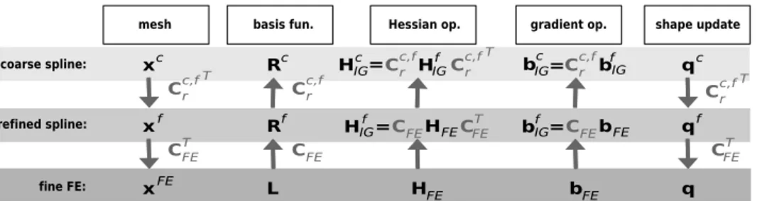
so that a unique basis is used for the representation of the surface at each multilevel step. An overview of the different transformations is given in Figure 4.

mesh basis fun. Hessian op. gradient op. shape update coarse spline: _xc xf xFE CT_FE Rc Rf L C_FE qc qf q C_FET Hf HFE H_FE C_FE C_FET refined spline: fine FE: bf bFE b_FE C_FE Hf = Hc= bf = bc= T C_rc,f C_rc,f IG IG T C_rc,f IG Cr c,f IG IG Cr c,f IG T C_rc,f

FIGURE 4 Overview of the different transformations enabling to communicate between the fine (analysis-suitable) FE mesh

and the different (multilevel) spline-based discretizations.

3.2.2

Construction: case of B-splines

In case of a B-spline geometric model, constructing 𝐂_{𝐹 𝐸}appears quite straightforward since both spline and FE discretizations rely on polynomials. Indeed, since the space generated by the B-Spline functions (smooth polynomials) is included into the one generated by the Lagrange functions (𝐶0_{polynomials), the process consists in extracting the smooth part of 𝐶}0_functions.

In order to form a multivariate 𝐶0mesh from a multivariate smooth B-spline mesh, the starting point consists in repeating all the inside knots of the knot-vectors until they reach a 𝑝 multiplicity. A specific knot-insertion process is thus performed which enables to get the famous Bézier extraction operator whose interest to relate IGA and FEA has been intensely demonstrated (see42,57,58,59,60_{to name a few). More precisely, the Bézier extraction operator maps a Bernstein basis onto a B-Spline basis.} Bernstein and Lagrange polynomials generates the same approximation subspace. Therefore, the second step consists in moving from the Lagrange basis to the Bernstein basis which can be easily performed by evaluating the Bernstein functions at the nodal points associated to the Lagrange basis. The succession of these two steps leads to the construction of the Lagrange extraction operator43_{that we denote 𝐃}

𝐿𝐴𝐺in the following. Consequently, we simply have 𝐂𝐹 𝐸 = 𝐃𝐿𝐴𝐺in case of B-splines. For more details regarding these transformations, the interested reader is advised to consult41,42,43.

Remark 6. Note that for better numerical efficiency, the Lagrange extraction operator can be directly computed from the B-spline and Lagrange basis. Indeed, it merely requires to evaluate the B-spline basis functions at the nodal points of the Lagrange basis.

Remark 7. The present work is restricted to quadratic functions since almost all standard FE codes do not go beyond second-order Lagrange finite elements (the famous 9-node quadrilateral element in 2D, or the 27-node cubic element in 3D). Nevertheless, we emphasize that the proposed methodology could be directly applied to higher-order spline-based discretization, provided that the corresponding higher-order FE are available in a FE-SDIC environment.

3.2.3

Construction: case of NURBS

As opposed to previous works on the subject that are restricted to B-splines40,18,19_{, we undertake to also consider NURBS here to} exactly represent conic sections. The Lagrange extraction can be extended to the case of NURBS but, it cannot directly go from a Lagrange basis to a NURBS basis since the first one is based on polynomials while the other one relies on rational functions. The NURBS version of the Lagrange extraction actually consists in mapping a rational Lagrange basis onto a NURBS basis, as detailed in43_{. To truly start with Lagrange polynomials, the construction of an additional mapping going from polynomials to} rational functions is required. Such a transformation cannot be exact since this is the space of the rational functions that includes the associated polynomials and not the other way around. A projection thus needs to be performed. In order to do so, we propose

to proceed as in41_{; that is, we start with the NURBS version of the Lagrange extraction and then perform the projection at the} Lagrange level. This offers the opportunity to follow a pragmatic yet accurate strategy.

More precisely, using the B-spline version of the Lagrange extraction operator and returning to (12), we can write:

𝐑𝑓(𝝃) = 𝐖 𝑓_𝐃

𝐿𝐴𝐺𝐋(𝝃)

𝑊𝑓_(𝝃) , (22)

where 𝐖𝑓 _{is the diagonal matrix collecting the weights of the refined NURBS discretization and 𝑊}𝑓_{(𝝃) =} ∑𝑛

𝑓 𝐼 𝐺 𝑘=1𝑤 𝑓 𝑘𝑁 𝑓 𝑘(𝝃) is the associated NURBS weight function. Omitting dependency on 𝝃, the NURBS weight function can be rewritten using the Lagrange basis as:

𝑊𝑓 = 𝑛𝑓_{𝐼 𝐺} ∑ 𝑘=1 𝑤𝑓_𝑘𝑁_𝑘𝑓 = (𝐰𝑓)𝑇𝐍𝑓 = (𝐰𝑓)𝑇𝐃_𝐿𝐴𝐺𝐋 = (𝐃𝑇_𝐿𝐴𝐺𝐰𝑓)𝑇𝐋= (𝐰𝐿𝐴𝐺)𝑇𝐋= 𝑊𝐿𝐴𝐺, (23)

where the weights associated to the rational Lagrange control points are:

𝐰𝐿𝐴𝐺= 𝐃𝑇_𝐿𝐴𝐺𝐰𝑓. (24)

The rational Lagrange functions are then defined as follows:

𝐑𝐿𝐴𝐺= 𝐖

𝐿𝐴𝐺_𝐋

𝑊𝐿𝐴𝐺 , (25)

where 𝐖𝐿𝐴𝐺_{is the diagonal matrix of the Lagrange weights. The link between NURBS functions and rational Lagrange} func-tions is finally made using Eqs. (25) and (23) in Eq. (22). Consequently, a new extraction operator 𝐃𝑊

𝐿𝐴𝐺is created as described below:

𝐑𝑓 = 𝐖𝑓𝐃_𝐿𝐴𝐺(𝐖𝐿𝐴𝐺)−1𝐑𝐿𝐴𝐺= 𝐃𝑊_𝐿𝐴𝐺𝐑𝐿𝐴𝐺. (26)

Then, going from 𝐋 to 𝐑𝐿𝐴𝐺_{or, in other terms, from 𝐱}𝐿𝐴𝐺_{(the location of the rational Lagrange control points) to 𝐱}𝐹 𝐸_{, can be} achieved very simply. Indeed, noticing that the control points of the rational Lagrange discretization interpolates the geometry, it appears possible to consider that the position of the FE nodes 𝐱𝐹 𝐸_{is exactly the same as the position of the rational Lagrange} control points 𝐱𝐿𝐴𝐺_{. Following this strategy, we end up with:}

𝐱𝐹 𝐸_≈(_𝐃𝑊 𝐿𝐴𝐺

)𝑇

𝐱𝑓 _{and 𝐑}𝑓 _{≈ 𝐃}𝑊

𝐿𝐴𝐺𝐋, i.e. 𝐂𝐹 𝐸= 𝐃𝑊𝐿𝐴𝐺. (27)

The above approximations get more accurate with the refinement of the NURBS mesh, which is assumed to be the case here since it is related to the last-level NURBS model. As demonstrated in41_{, this process provides sufficient accuracy with already} rather coarse NURBS meshes for typical engineering geometries.

3.3

Proposed methodology

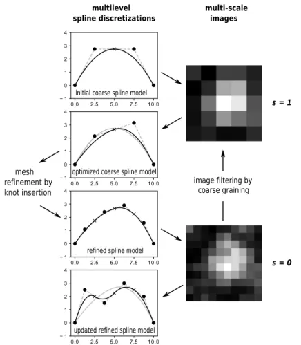
We now have all the ingredients in hand to present the proposed methodology. The objective is to improve the mesh-based shape measurement occurring in FE-SDIC by using, in a non-invasive manner, a geometrically sound regularization. In order to do so, the main idea is to relate the multilevel spline parametrizations of the geometry (and of its update) with the multi-scale images used for the initialization of the shape measurement (see remark 3). The principle is illustrated in Fig. 5. The different approximation subspaces that describe the geometry are chosen in accordance with the resolution of the images so that the shape measurement problem is regularized at each scale (number of DOF versus number of pixels). The coarse scales enable to fit the major tendencies of the surface while the finer ones allow the representation of sharper variations. Moving from scale 𝑠 to finer scale 𝑠 − 1, the spline design space is enhanced while keeping the same geometry, and the initial solution for the shape measurement problem of scale 𝑠 − 1 is taken as the final solution of scale 𝑠.

Remark 8. In practice, the method starts from a sufficiently coarse representation of the nominal geometry. So far, in experi-mental mechanics, specimen’s shape is relatively smooth such that very compact spline representations with very few DOF are generally sufficient. In a situation where the initial CAD representation should be too fine to effectively regularize the problem, it would be possible to either reduce the number of scales or resort to additional Tikhonov-type regularization techniques. Note that even in such a case, although insufficient a certain amount of geometric regularization is expected. Indeed, the level of Tikhonov regularization should presumably be lower than the one which would be required with an analysis-suitable FE mesh.

initial coarse spline model

optimized coarse spline model

refined spline model

updated refined spline model mesh refinement by knot insertion image filtering by coarse graining multilevel spline discretizations multi-scale images s = 1 s = 0

FIGURE 5 Principle of the geometric regularization: the multilevel spline optimization process is coupled with the multi-scale

initialization of shape measurement.

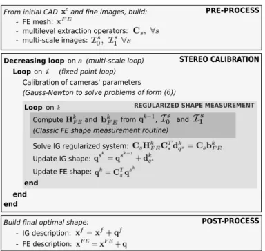
More precisely, an overview of the proposed regularization scheme included in the calibration of the whole stereo rig is given in Fig. 6. For simplicity, we denote by 𝐂_𝑠the extraction operator that maps the fine FE space onto the spline discretization of scale 𝑠, i.e. 𝐂_𝑠is defined such that:

𝐂₀= 𝐂𝐹 𝐸 and 𝐂𝑠= (_𝑠−1 ∏ 𝑖=0 𝐂(𝑠−𝑖),(𝑠−𝑖−1)_𝑟 ) 𝐂_{𝐹 𝐸}, ∀𝑠 ∈{1, .., 𝑛𝑠 } , (28)

where 𝑛_𝑠is the number of scales and 𝑠 = 0 corresponds to the finest scale while 𝑠 = 𝑛_𝑠refers to the coarsest scale. As can be observed, making use of the IG-FE bridge of previous section, the implementation is performed from standard FE-SDIC routines with minimal effort. Summarizing, we proceed as follows for the regularization. From the initial CAD representation of the theoretical surface, we build in the pre-processing step a fine analysis-suitable FE mesh and the different multilevel spline discretizations through their corresponding extraction operators 𝐂_𝑠. Then, entering into the shape measurement loop and beginning with the coarsest scale, we project, at each iteration of the Gauss-Newton solver, the FE hessian and gradient onto the first-level spline space and solve the associated regularized IG system. We thus end up with the IG shape update that can be converted in terms of nodal FE shape update so that the FE hessian and gradient can be updated for the next iteration. Going to the finest scale, we finally repeat the previous procedure with the different refined spline spaces to regularize at each scale. The final shape can be given either in terms of splines (thereby directly compatible with CAD environments) or in terms of finite elements (thus facilitating the communication with numerical simulations).

STEREO CALIBRATION

REGULARIZED SHAPE MEASUREMENT

PRE-PROCESS From initial CAD and fine images, build:

- FE mesh:

- multilevel extraction operators: - multi-scale images:

Decreasing loop on (multi-scale loop)

Loop on (fixed point loop) Calibration of cameras' parameters

(Gauss-Newton to solve problems of form (6))

Loop on

Compute and from , and (Classic FE shape measurement routine) Solve IG regularized system:

Update IG shape: Update FE shape: end end end POST-PROCESS

Build final optimal shape: - IG description: - FE description:

FIGURE 6 Overview of the proposed regularization scheme included in the calibration of a stereo rig.

4

EXAMPLES

In this section, the proposed regularization technique for mesh-based shape measurement is applied to a real experiment. A steel open-hole tensile specimen of size 180 × 50 × 2 mm and hole diameter 28 mm was considered. A dedicated speckle pattern was laser printed over a layer of uniform white paint. A pair of 5 Mpx CCD cameras and 50 mm lenses was used to capture the 8bit 2452x2052 digital images presented in Figure 1. The stereo-angle was set around 25◦_{which represents a good compromise} between in-plane and out-of-plane uncertainties61. The intrinsic parameters of the nonlinear camera models (first order radial distortions) were calibrated prior to the experiment using a series of digital images of a calibration target made of a grid of 12x9 dots with a step size of 3 mm. The obtained intrinsic parameters are considered fixed in the remainder of the study. More precisely, two configurations were considered for the study:

• In a chronological order, the specimen was first clamped in the lower jaw of an electro-mechanical tensile testing machine. The upper part of the specimen was left free. In this first configuration, a set of images was taken and is referred to as the flat configuration, as the observed surface of the specimen was almost plane. This configuration is used to analyse the robustness of the method to a reasonably complex shape.

• The specimen was then clamped in the upper jaw. Since the jaws are slightly misaligned, the hyper-static clamping gener-ated a torsional moment and the specimen twisted. The misalignment was around 2 or 3◦_{which should generate significant} waviness. The corresponding set of images is referred to as the twisted configuration. With this case study, it is possible to analyze the method in a configuration where the difference between the theoretical (considered flat) and real (twisted) shapes is significantly greater than in standard mechanical experiments.

For a clear understanding of the results, we choose in the following to start with the twisted configuration and then turn to the flat configuration. The two pairs of digital images are analysed by (a) the proposed geometric, Bézier-based, regularized shape measurement method, (b) a standard FE-based shape measurement possibly considering Tikhonov regularization and (c) a more standard subset-based DIC method. It must be mentioned, at this stage, that the regions of interest of the FE-based and subset DIC are not equal. Indeed, the FE (or IG) meshes do conform to the edges of the specimen, whereas subset DIC was not able to perform shape measurement too close to the boundaries. This point should be kept in mind when comparing global and local DIC solutions.

4.1

Pre-processing: construction of the geometric model and FE mesh

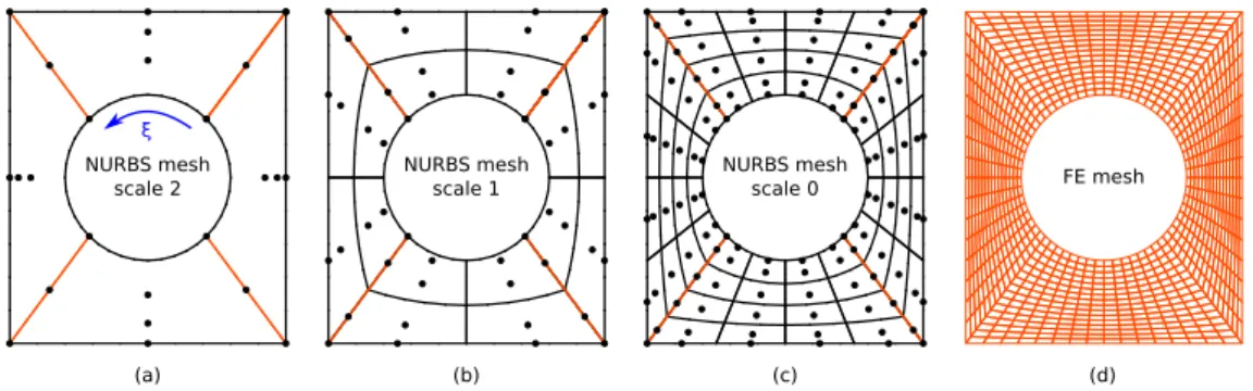
The nominal geometry of the sample consists in a plate with a circular hole. As a result, its exact representation in CAD requires the use of NURBS (rational B-splines). It is common to proceed as in Figure 7(a) for the building of the first NURBS model of such a geometry. Given that the four vertices of the plate imply a 𝐶0 _{regularity of the geometry at} those points, the coarsest NURBS model necessarily involves 4 𝐶0-𝐶0 elements. More precisely, denoting by 𝜉 the param-eter describing the circumferential direction, we needed to start with degree 𝑝 = 2 in that direction with knot-vector Ξ = {0, 0, 0, 0.25, 0.25, 0.5, 0.5, 0.75, 0.75, 1, 1, 1} (for more details on NURBS constructions, see, e.g.,33). Along the other direc-tion, even if degree 1 would be sufficient, we also took degree 2 so as to be consistent with the final FE-mesh that is made of standard 9-node (i.e. bi-quadratic) elements. Starting with the NURBS model composed of 4 quadratic elements, we thus only performed knot-insertion (inserting one knot at a time) to get the different (multilevel) NURBS parametrizations (see Figs 7(b) and (c)). We finally further carried out knot-insertion and applied the IG-FE mapping of section 3.2 (see Eq. (17)) to obtain the analysis-suitable FE-mesh (see Figure 7(d)).

FIGURE 7 Initial CAD parametrization, mutli-level NURBS meshes and final fine FE mesh. The 𝐶0_{lines are orange. The final}

FE mesh is composed of 1000 elements.

Remark 9. Let us recall here that although a NURBS parametrization is used to represent exactly the in-plane geometry, the shape optimization with the proposed strategy only acts on the out-of-plane locations of the control points (see remark 4). As a result, the modification of the shape should not be interpreted as a NURBS modification but rather as some "spline" modification with fixed weights. We believe that the measurement uncertainties must certainly be greater than the difference between NURBS and B-Spline modifications. Now, given that the computational cost associated to 𝐃_𝐿𝐴𝐺and 𝐃𝑊

𝐿𝐴𝐺is similar (only two additional diagonal-matrix/matrix products for 𝐃𝑊_𝐿𝐴𝐺, see Eq. (26)) and that we simply have a practical NURBS parametrization of the nominal plate with a hole, we decided to use a NURBS instead of an approximate B-Spline parametrization for the nominal geometry here.

4.2

Results : twisted configuration

Let us recall that, because of the misalignment of the jaws, in this clamped-clamped configuration, the specimen underwent a significant twist. Note that theses images were not analysed for displacement measurement using FE-SDIC with respect to the flat configuration images. They were used for shape measurement independently as if this configuration was the initial state of the specimen.

4.2.1

Classic FE-based shape measurement without any regularization

A first classic FE shape measurement was performed using the FE mesh given in Figure 7(d) without any regularization. The obtained shape is represented in Figure 8. In order to compare the shape measurements obtained with the different considered techniques, we chose the color data to represent the distance to the best fitting plane (BFP) instead of directly plotting the shape correction field 𝐒(𝐗) which would not be available using the subset approach. The shape is typical of a twist test. The waviness is around one millimeter, which, at the scale of this specimen, is large. In addition, the resulting shape is relatively noisy. Even tough the noise is one order of magnitude smaller than the artificially large shape correction field, it still seems large and unphysical.

FIGURE 8 Twisted specimen: shape obtained with classic FE-SDIC without regularization (def. scale fact. x30).

4.2.2

Use of standard Tikhonov regularization

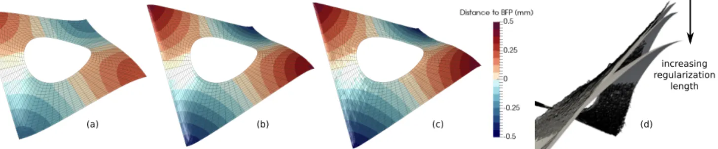
In order to regularize this noise, a classic Tikhonov regularization technique was first considered. The shape obtained for three different regularization lengths is given in Figure 9. As expected, using Tikhonov regularization, the shape measurements

FIGURE 9 Twisted specimen: shape obtained using a classic FE-SDIC with Tikhonov regularization for different values of the

regularization length: decreasing values of the regularization length from (a) to (c) respectively (def. scale fact. x30).

appeared clearly smoother, especially for large values of the regularization length (see Figs. 9(a) and (b)). It can be seen that such high levels of regularization may also affect the shape. Indeed, on Figure 9(d), the influence of the regularization length on the shape is depicted, with the subset approach as the reference. Using a too large regularization length reduces the displace-ment magnitudes and underestimates the shape waviness. Asymptotically, using very large values of regularization would lead to an almost constant correction field, which would correspond to a rigid body translation of the observed surface with respect to the theoretical CAD.

Conversely, for lower values of the regularization length, the solution looks more like the shape obtained without regulariza-tion. For instance Shape 9(c) is less noisy than the one illustrated in Figure 8, but high frequency noise is still present, which means that the regularization was still not sufficient. Even in this case, where the regularization level was insufficient to get completely rid of noise, it can be observed on Figure 9(d) that the correction field at the top corner was already underestimated because of the differential nature of the chosen regularization term. As shown in this example, choosing the correct regulariza-tion length value may become a tricky trade-off. In other words, a satisfying value of the regularizaregulariza-tion length may not exist, as it seems to be the case here.

4.2.3

Use of the proposed geometric regularization

Next, the proposed geometric regularization scheme was considered with the same image set. The multi-scale initialization technique described in section 3.3 was applied with three scales using the three NURBS meshes of Figure 7. The corresponding shapes obtained at each scale are given in Figure 10.

FIGURE 10 Twisted specimen with the proposed geometric regularization (def. scale fact. x30).

First, it can be observed that the shapes obtained at the three scales are very smooth. Indeed, the very low-dimensional spline approximation subspace acts as a very strong regularization technique. Each of the three shapes are very similar to each other and also in good agreement with the shape provided by the subset DIC method. In addition, the reduction in the correction field’s magnitude observed when using the Tikhonov regularization did not occur here. Even at the highest scale, where the spline representation is particularly coarse, a very good approximation of the shape was already obtained. This property of the geometric regularization is particularly interesting for the highest scales of the multi-scale approach, since they are associated to high regularization levels.

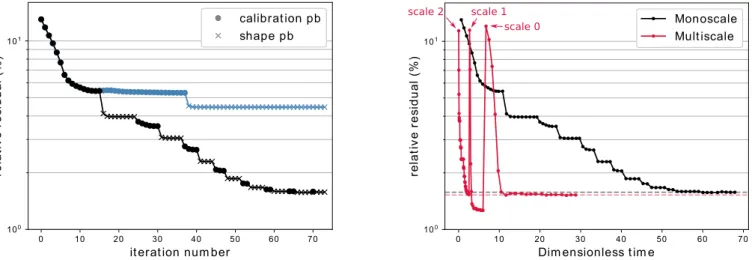
Figure 11(left) presents the evolution of the standard deviation of the graylevel residual field in percent of the reference image dynamics (later denoted relative residual) as a function of the iteration number. It compares the convergence of the problem

FIGURE 11 Convergence of the algorithm on the twisted use case: (left) convergence (vs iterations) of the relative residual with

(black) and without (blue) the fixed point iterations and (right) convergence speed (vs dimensionless time) for the monoscale and multi-scale approaches.

It can be seen that, at least on this case, converging the fixed point algorithm (by alternating between calibration and shape problems) is mandatory to converge towards an accurate solution. It is the case here because the actual shape is significantly different from the initial CAD. On the (right) side of the same figure, the relative residual is plotted as a function of the CPU time normalized by the CPU time taken by one iteration at scale 0, for the monoscale (only scale 0) and multi-scale approaches. It can be seen that, although the number of iterations may increase, the computational time is clearly reduced (divided by 2 in this case), since the higher scales are associated to low definition images whose interpolation is far cheaper. Note also, that when using the multi-scale approach, the value of the relative residual was lower than that of the monoscale alternative. Lower relative residual emerges from the fact that the multiscale initialisation, in addition to convergence acceleration, was designed to avoid local minima. In this example, the solutions seem to be similar, but the multi-scale approach, by avoiding local minima, may allow to reduce significantly the relative residual and therefore improve the measurement accuracy.

Remark 10. Note that the residual at scale 𝑠 > 0 was estimated using the coarsened images and not with the full resolution (scale 0) images, for efficiency. This explains why the estimated residual at scale 𝑠 > 0 is sometimes a little smaller than the one at scale 0 after convergence on Figure 11(right).

4.2.4

A note regarding brightness and contrast correction

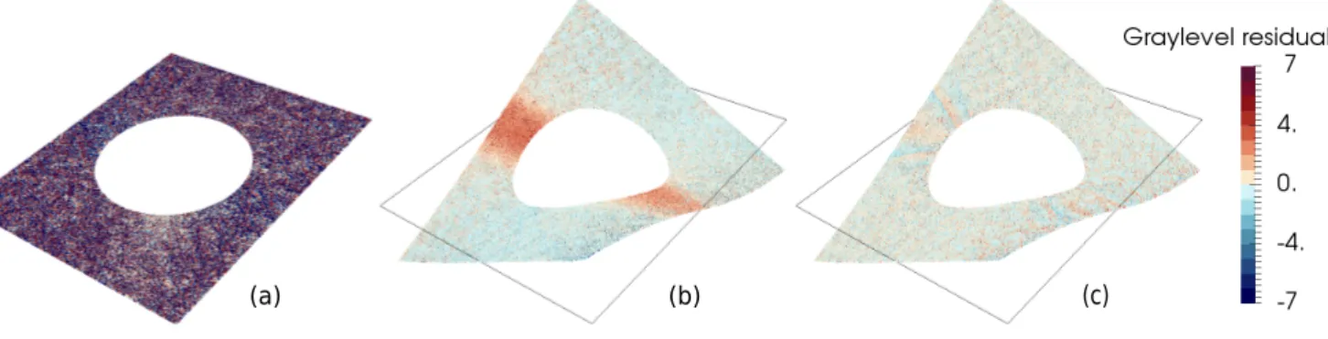
Another interesting point with this test case is the analysis of the graylevel residual field 𝑟(𝐒(𝐗), 𝐩) at scale 𝑠 = 0 before and after convergence, with and without elementary brightness and contrast correction. First, the initial graylevel map, obtained with the initial CAD (flat) shape and the initial set of extrinsic parameters, is depicted in Figure 12. Its value is about 70% of the

(a) (b) (c)

FIGURE 12 Graylevel residual 𝑟(𝐒(𝐗), 𝐩) in percent of the dynamic of the images with (a) the initial CAD shape and after

convergence (b) without and (c) with elementary brightness and contrast correction (def. scale fact. x30).

dynamic of the image which means that the graylevels do not correspond at all. After 8 iterations of the fixed point algorithm, the graylevel residual dropped to less than 10% of the images dynamic. It means that the graylevel conservation was correctly verified. It can be seen on Figure 12(b) that the residual map presents a band of higher value located around the hole when using a global brightness/contrast correction. This localized bad verification of the graylevel conservation was attributed to the presence of a specular reflection of the light which seems consistent with the twisting of the specimen. This phenomenon locally modifies the brightness and contrast (B/C). As shown here, global B/C correction methods can not take this into account. The proposed elementary B/C correction method (see remark 2) was applied and the resulting graylevel residual is depicted on Figure 12(c). It presents a homogeneous value around 2% of the dynamic in all the region of interest. This elementary correction technique is very simple but generic. It was shown that it can efficiently account for a complex local B/C variations which would be difficult using a global descriptor.

4.3

Results : flat configuration

In this section, the so-called flat configuration where the specimen is clamped at the bottom end only is being analysed. Since here the specimen is nearly flat, the shape correction field is expected to be of lower magnitude, but less regular than the twist

of the previous section. Only the final shape measurements are plotted in this section to study the robustness of the geometric regularization method with respect to a more complex shape with lower signal to noise ratio. Figure 13 presents the shape measurement and distance to BFP when using (a) the FE-SDIC approach without regularization, (b) the local SDIC method and (c) the geometric regularization technique. First it can be noticed that all the shapes are in good agreement with each other. Note

FIGURE 13 Flat specimen shapes with distance to best fitting plane (BFP) in mm: (a) measured by the FE-SDIC without

regularization, (b) measured using the subset based SDIC and measured using the proposed geometric regularization: (c) Spline parametrization of the optimal shape and (d) corresponding measured finite element mesh (def. scale fact. x300).

that the waviness is one order of magnitude smaller than in the twist case. The FE and local SDIC measurements are clearly affected by noise. The geometric regularization technique efficiently manages to extract a regular shape from the images. From this measurement which provides the NURBS parametrization of the optimal shape, and using the IG-FE bridge of section 3.2, it is possible to build directly the FE mesh (see Figure 8(d)) which exactly corresponds to the same shape. Such an output may be convenient to be used for FE-SDIC displacement measurements in the context of validation/identification of FE models.

5

CONCLUSION

In this paper, we developed a hybrid IG-FE strategy for the regularization of the mesh-based shape measurement occurring in FE-SDIC. From a regularization point of view, the proposed strategy draws inspiration from the techniques developed recently in the isogeometric shape optimization community, especially with the multilevel design concept36,37,38_{. By making use of the} advanced spline refinement procedures and of adequate Bézier-based operators, the main idea here was to extract, from the initial FE subspace, smoother multilevel spline parametrizations of the geometry and to relate them with the multi-scale images used for the initialization of shape measurement. This treatment enabled to efficiently regularize, with a geometrical meaning, the problem at each scale. From a practical point of view, the proposed approach consists of nothing more than projecting the