Ammonia at Blodgett Forest, Sierra Nevada, USA

HAL Id: hal-00303116

https://hal.archives-ouvertes.fr/hal-00303116

HAL is a multi-disciplinary open access

archive for the deposit and dissemination of sci-entific research documents, whether they are pub-lished or not. The documents may come from teaching and research institutions in France or abroad, or from public or private research centers.

L’archive ouverte pluridisciplinaire HAL, est destinée au dépôt et à la diffusion de documents scientifiques de niveau recherche, publiés ou non, émanant des établissements d’enseignement et de recherche français ou étrangers, des laboratoires publics ou privés.

Ammonia at Blodgett Forest, Sierra Nevada, USA

M. L. Fischer, D. Littlejohn

To cite this version:

M. L. Fischer, D. Littlejohn. Ammonia at Blodgett Forest, Sierra Nevada, USA. Atmospheric Chem-istry and Physics Discussions, European Geosciences Union, 2007, 7 (5), pp.14139-14169. �hal-00303116�

ACPD

Full Screen / Esc

Printer-friendly Version Interactive Discussion

EGU Atmos. Chem. Phys. Discuss., 7, 14139–14169, 2007

www.atmos-chem-phys-discuss.net/7/14139/2007/ © Author(s) 2007. This work is licensed

under a Creative Commons License.

Atmospheric Chemistry and Physics Discussions

Ammonia at Blodgett Forest, Sierra

Nevada, USA

M. L. Fischer and D. Littlejohn

Environmental Energy Technologies Division, E.O. Lawrence Berkeley National Laboratory, 1 Cyclotron Rd., Berkeley CA, 94720, USA

Received: 5 September 2007 – Accepted: 27 September 2007 – Published: 5 October 2007 Correspondence to: M. L. Fischer (mlfischer@lbl.gov)

ACPD

Full Screen / Esc

Printer-friendly Version Interactive Discussion

EGU

Abstract

Ammonia is a reactive trace gas that is emitted in large quantities by animal agriculture and other sources in California, which subsequently forms aerosol particulate matter, potentially affecting visibility, climate, and human health. We performed initial measure-ments of NH3at the Blodgett Forest Research Station (BFRS) during a two week study 5

in June, 2006. The site is used for ongoing air quality research and is a relatively low-background site in the foothills of the Sierra Nevada. Measured NH₃mixing ratios were quite low (<1 to ∼2 ppb), contrasting with typical conditions in many parts of the Central

Valley. Eddy covariance measurements showed NH3fluxes that scaled with measured NH₃ mixing ratio and calculated aerodynamic deposition velocity, suggesting dry de-10

position is a significant loss mechanism for atmospheric NH₃at BFRS. A simple model of NH3 transport to the site supports the hypothesis that NH3is transported from the Valley to BFRS, but deposits on vegetation during the summer. Further work is nec-essary to determine whether the results obtained in this study can be generalized to other seasons.

15

1 Introduction

In California and the nation, many areas are out of compliance with federal particulate matter standards designed to protect human health (NRC 1998; NRC 2000). Nation-ally, Congress has set a goal to remediate current and prevent future impairment of vis-ibility in over 150 federally designated Class 1 Federal (Malm et al., 2000) designated 20

sites. Ammonia (NH3) is the primary gas to form aerosols in combination with acidic species (e.g., SOx, NOx) that are produced in combustion processes from energy re-lated activities. While mixing ratios of combustion derived species are regure-lated, NH₃ is not. If ammonia limits aerosol concentrations, then controls on emissions of NOx and perhaps SOx may not be effective in controlling aerosol concentrations, visibility, 25

ACPD

Full Screen / Esc

Printer-friendly Version Interactive Discussion

EGU The magnitude of NH3 fluxes are expected to vary enormously over space. NH3

is emitted from strong point sources (e.g. animal agriculture), medium strength dis-tributed sources (e.g., fertilized fields and automobile catalytic converters), and ex-changed with spatially vast areas of soil and vegetation (Potter et al., 2001; Kirchstetter et al., 2002; Battye et al., 2003). Ammonia is of particular interest in California because 5

it is emitted in large amounts from agricultural sources in the Central Valley, leading to high (20–40 ppb) surface layer NH3 mixing ratios (Fischer et al., 2003; Lunden et al., 2003; Chow et al., 2006). For example, recent work suggest that San Joaquin Valley area emissions might range from 8 to 42 g N ha−1day−1 (11 to 50 ng NH3m−2 s−1) in winter and summer respectively, with approximately 78 % of the summertime emissions 10

derived from animal agriculture (Battye et al., 2003).

While most NH3measurements have been made in urban areas in California, some measurements have been made in rural settings. Airborne measurements in the af-ternoon mixed layer showed that ammonium compounds (i.e., NH_{3 + NH}+₄) were the dominant component of the N budget with variable NH3 concentrations corresponding 15

to mixing ratios of 10±7 and 2.5±0.5 ppb in boundary layer above the foothills of the Sierra in the boundary layer above Lake Tahoe respectively (Zhang et al., 2002). In contrast, a ground-based study at Lake Tahoe measured significantly lower concen-trations corresponding to approximate mixing ratios between 0.6 to 1.5 ppb and mean summer deposition rates between 3 to 11 ng N m−2 _s−1 _{(Tarnay et al., 2001). The} pre-20

vious work raises the question of whether there are vertical gradients in NH3 caused by dry deposition or whether the differences in NH3at the surface and aloft are due to different measurement times.

Here we describe a short term study of the NH3 mixing ratios and NH3 fluxes at a rural site in the foothills of the Sierra Nevada.

25

ACPD

Full Screen / Esc

Printer-friendly Version Interactive Discussion

EGU

2 Methods

The methods section includes a description of the measurement site, the fast response NH3instrument, the methods used for data reduction, a filter sampling system used to provide comparative NH₃measurements, a method used to calculate the aerodynamic deposition velocity expected under different meteorological conditions, and a predictive 5

model for NH3mixing ratios at the measurement site. 2.1 Measurement Site

2.1.1 UC Berkeley Blodgett Forest Research Station

We measured NH3 mixing ratios and fluxes near the University of California’s Sierra Nevada the Blodgett Forest Research Station (BFRS), located west of the Sacramento 10

region as shown in Fig. 1. The BFRS site is an attractive site for this work because it is representative of large areas of forested land with acidic soils in the mountainous Western US and has been the site of ongoing air quality measurements (Goldstein et al., 2000; Dillon et al., 2002; Kurpius et al., 2002; Farmer et al., 2006). Although recent work at BFRS has studied mixing ratios and fluxes of several reactive nitrogen species, 15

NH3has not been measured previously.

The BFRS tower is located at 38.88◦_{N, 120.62}◦_{W, at an elevation of 1315 m in a} re-growing ponderosa pine plantation. Tree heights ranged from approximately 8–10 m. Terrain is gently sloping downward from east to west. Power to the site is provided by a diesel generator located approximately 130 m due north of the tower site. The 20

predominant winds are upslope from the southwest during the day and downslope from the northeast during the night.

2.2 NH₃instrument

Ammonia was measured using a sensitive fast-response quantum-cascade laser (QCL) spectrometer operating at a frequency of 965 cm−1 _{(Aerodyne Research Inc} 25

ACPD

Full Screen / Esc

Printer-friendly Version Interactive Discussion

EGU (ARI), similar to that used for eddy covariance flux measurements of NO₂ (Zahniser

2003; Horii et al., 2004). The precision of the NH3 instrument is normally 0.3 ppb (1 sigma) for data collected at a frequency of 10 Hz. The instrument provided highly auto-mated control of high frequency data collection, zero adjustments, and zero and span checks as described below using a dedicated software package (TDLWintel).

5

In addition to the QCL spectrometer, additional data was collected. First, a sonic anemometer (Gill Windmaster Pro) was used to measure fluctuations in virtual air tem-perature and 3-D winds. The digital output from the anemometer was logged by the computer controlling the QCL spectrometer. The anemometer was physically posi-tioned so that the sensing volume was located 30 cm from the inlet manifold of the 10

NH₃ instrument. Second, a data logger (Campbell CR23X) recorded gas flow rates controlled by mass flow controllers, inlet surface temperatures measured with thermo-couples, atmospheric temperature and relative humidity (Vaisala Y45), and short wave solar radiation (Kipp and Zonen CM3).

The NH3and ancillary meteorological measurements were made at a height of ap-15

proximately 10 m above the ground, sufficient to reach slightly above the nearby veg-etation. The combined weight of the spectrometer, support electronics and thermal control system and liquid nitrogen storage dewar for automated refills of the spectrom-eter detector dewar (total of ∼200 kg) required a platform scissor-lift. The scissor lift was located at a distance of approximately 8 m from the main BFRS meteorological 20

tower. During the two day period from 24 to 25 July, when the LBNL measurements were compared with the filter sampler, the platform was lowered to a height of ∼6 m to match the height of the filter sampler. The filter sampler was deployed on the main BFRS tower.

To achieve high temporal resolution necessary for eddy covariance measurements, 25

we designed a high flow rate gas sampling and calibration subsystem that transmits ambient NH3 vapor to the spectrometer with minimal residence time. A schematic of the inlet and calibration system is shown in Fig. 2. A flow of ambient air is drawn into the sample manifold by the combination of a manifold flow pump (at 20 slpm) and

ACPD

Full Screen / Esc

Printer-friendly Version Interactive Discussion

EGU into the NH3 spectrometer at a rate (approximately 25 slpm) determined by the pump

speed (Varian 600 dry scroll) and the diameter of a critical orifice inlet. After entering the critical orifice (which reduces the pressure to approximately 50 Torr), air is passed through a 0.2 micron PTFE air filter (Gelman PALL, Acro-50), a 2 m long 1 cm diameter PFA Teflon tube to the multipass optical cell contained within the QCL spectrometer. 5

All glass surfaces are siloxyl coated (General Electric) and surfaces are heated as suggested in Neuman et al. (1999). In our application, the temperatures of the different inlet parts were maintained between 40 and 45◦_{C by a set of four temperature control} circuits, while the optical bench including the optical absorption cell was maintained at 30◦C.

10

During the measurements, the instrument zero was adjusted every 30 min, under control of the spectrometer computer, by overfilling the inlet manifold with an approx-imately 60 slpm flow of dry nitrogen supplied by a large liquid N2 supply dewar. Typ-ically, zero adjustments were significantly less than 1 ppb. In addition, the instrument zero and span were checked periodically. Zeros were generally checked every 30 min. 15

The span of the instrument was checked by reversing a backflow of 300 sccm that normally removes a 100 sccm flow of NH₃ supplied from a permeation tube source. After applying NH3for 30 s, the backflow is reestablished removing NH3from the inlet. The response time of the instrument to an approximately 15 ppb step in NH3 mixing ratio was checked once each hour by applying a NH₃from a permeation tube source 20

to the N2 flow. As shown in Fig. 3, the response is well characterized by the sum of exponential decay terms as

NH₃(t) = No(a1exp(−t/τ1) + a2exp(−t/τ2)), (1)

where a_{1 = 0.8 +/−0.05, τ1 = 0.35 +/− 0.05 s, a2 = (1-a1}), andτ2 = 4 +/−1 s. The uncertainties in the values reported for the decay coefficients time constants represent 25

ACPD

Full Screen / Esc

Printer-friendly Version Interactive Discussion

EGU 2.3 Data reduction

The 10 Hz data NH3 were processed to estimate mean NH3 mixing ratios and NH3 fluxes. For mean NH3, a continuous estimate of instrument zero was estimated as a spline interpolation of NH₃ values obtained during the stable period at the end of zero checks (see Fig. 3). The instrument zero was less than 1 ppb for 90% of the 5

data, until 21 June, when the instrument ran out of cryogens. Upon restarting the instrument on 23 June, the instrument noise level had increased by nearly an order of magnitude (to ∼3 ppb in 1 s integration), leading to a larger variation in zero level. Following subtraction of instrument zeros, mean mixing ratios were calculated for 1 and 12 h bins.

10

NH3 flux was computed for 1/2 h intervals from the covariance of the 10 Hz NH3 mixing ratios and the vertical wind using standard techniques (Baldocchi et al., 1988). Wind fields were rotated to a coordinate system with zero mean vertical wind. Fluc-tuations in ammonia, NH3’, virtual temperature, T’, and wind vectors, u’, v’, and w’, were calculated by subtracting 1/2 hour block averages. Vertical fluxes were calculated 15

as the covariance between vertical wind fluctuations, w’, and other quantities. Peri-ods during NH3zero or span measurements were excluded. The mean ammonia flux, FNH3 =<w’NH3’> was estimated 1/2 h interval. The time lag between w’ and NH3’, required to maximize F_NH3, was determined from lag correlation plots. Typical values for the best lag were small (<0.3 s), and roughly consistent with that expected from the

20

measured step response of the inlet system.

To correct for loss of high frequency NH₃ fluctuations due to finite frequency re-sponse of the gas inlet, we applied an empirically derived multiplicative correction (Horii et al., 2004). The correction was computed from the measurements of sensi-ble heat obtained from the sonic anemometer. Here sensisensi-ble heat is calculated as, 25

H=ρCp <w’T’>, where ρ and Cp are the density and specific heat of air respectively. We calculated the correction factor,

fcorr= w′T′/w′Tsm′ , (2)

ACPD

Full Screen / Esc

Printer-friendly Version Interactive Discussion

EGU where Tsm′, is obtained by convolving T’ with the double exponential decay function

de-scribing the step response to NH₃span decay in Eq. (1). Typical values for F_corrranged from 1 to 1.2 depending on the atmospheric stability, indicating that the NH3 captured most of the high frequency fluctuations contributing to the flux. As an additional check of the frequency response, power spectra for w’T’, w’T_sm′_{, and w’NH}

3’ were computed 5

for 1/2 h periods and compared with the −4/3 power law expected from Komolgorov similarity theory.

We determined whether the NH₃fluxes were stationary by comparing the 1/2 h mean flux with the mean of the individual fluxes determined from 5 min sub-intervals. Data was considered to be stationary when the flux calculated from the subintervals is within 10

30% of the 1/2 h mean flux (Foken et al., 1996). Non-stationary conditions typically occur during periods of intermittent turbulence which typically occurs on nights when the air is stably stratified and friction velocity, u*=<−w’u’>1/2 is low (u*<0.1 m s−1_). Non-stationary fluxes of nitrogen oxides have also been observed at BFRS, associated with emissions from the generator (Farmer et al., 2006). We excluded the data (∼20%) 15

obtained when the wind direction was within 45 degrees of north. 2.4 Filter sampling

Ambient NH3 concentrations were determined during a two day period (starting on the evening of 23 June and continuing into midday of 25 June) using filter samples collected with the Desert Research Institutes (DRI) sampler (Chow et al., 1993). As 20

described above, the inlet of the filter sampler was located at a height of 5.5 m off the ground on the main meteorological tower. In this method, two filter samples are col-lected simultaneously. One filter is exposed to a flow of ambient air, while the other is exposed to air that has had gaseous NH3 removed by an annular denuder. Then the denuded filters collected only particulate NH+₄, while the undenuded filter collected 25

both gas and aerosol. Gaseous NH₃ is estimated as the difference between unde-nuded and deunde-nuded measurements. In this experiment, four sets of paired (deunde-nuded

ACPD

Full Screen / Esc

Printer-friendly Version Interactive Discussion

EGU and undenuded) citric acid coated filters were exposed to air flows near 100 liters per

minute (measured before and after each sample was collected) over the two day pe-riod using 12 h collection times (18:00–06:00 and 06:00–18:00 PDT, or 01:00–13:00 and 13:00–01:00 GMT). Before and after sample collection the filters were stored in capped, bagged, and stored in an ice chest. Following collection on 25 June, the sam-5

ples were returned to DRI for analysis of NH+₄ ions captured on the citric acid. 2.5 Estimate of maximum deposition velocity

As a check on the observed NH3 fluxes, we computed deposition velocities, Vd = F_NH3/NH₃, for each 1/2 h interval and compared it to a simple model for the maximum deposition velocity expected if all NH3 molecules are reaching the leaf surfaces are 10

adsorbed. In general, deposition velocity can be expressed in a resistance based model as,

Vd= (Ra+ Rb+ Rc)−1, (3)

where Ra, Rb, and Rc are the aerodynamic, leaf boundary layer, and stomatal resis-tances respectively. In the limit that the vegetation is nitrogen limited and readily ac-15

cepts all NH₃reaching the leaf surface, R_ccan be assumed to be small and a maximum deposition velocity can be written as

Vdmax = (Ra+ Rb)−1, (4)

Using standard turbulence models for the surface layer fluxes, one can write a set of expressions for Raand Rb(Wesely 1989; Horii et al., 2004). Here

20

Ra= u/u ∗2−χH/(ku∗), (5)

where k is the Von Karmen coefficient (∼0.4). Under stable conditions χH can be expressed as

χH= 5(z − d)/L, (6)

ACPD

Full Screen / Esc

Printer-friendly Version Interactive Discussion

EGU where z is the measurement height, d is the displacement height (often assumed to be

0.75 vegetation height), and L is the Monin–Obukhov length scale, L=−kg<w’T’>/Tu*3, and g is the acceleration due to Earth’s gravity. Stable conditions are defined as when L>0. Under unstable conditions (L<0),

χH= exp(0.598 + 0.39 ∗ ln(−(z − d)/L) − 0.09 ∗ (ln(−(z − d)/L))2). (7) 5

Finally, the boundary layer resistance at the leaf surface can be written as

Rb−1∼ u∗/7.1 (8)

Under the conditions observed at a mixed deciduous forest in Northeastern United States, Horri et al. (2004) observed 0.01<Vd<0.08 ms−1.

2.6 Simulation of NH₃mixing ratios 10

Measured NH3 mixing ratios were compared with simulated NH3 concentrations de-rived from and a regional emission inventory estimate of NH₃emissions combined with a particle back trajectory calculation of time and space specific surface influence on atmospheric gas concentrations and dry deposition of NH3.

A simple NH₃ emission model was used for these simulations. NH₃ emissions for 15

June were estimated assuming that cows in dairies and feedlots generated a large fraction of the emissions in the Central Valley. The spatial distribution of cows was obtained from county level statistics for 2002 animal stocking density reported by the United States Department of Agriculture’s National Agricultural Statistics Service (NASS, 2004). We estimated the NH3 emission factors for the summer conditions by 20

scaling the annual averaged emissions factors by the ratio (2.3) of summer time ani-mal fluxes to annually averaged aniani-mal fluxes in the San Joaquin Valley (Battye et al., 2003). The resulting emissions factors are 185 and 64 g NH3animal−1 day−1 for dairy and non-dairy cattle respectively. County level NH3 fluxes were calculated as the to-tal NH₃ emissions for each county normalized by the area and are shown in Table 1. 25

ACPD

Full Screen / Esc

Printer-friendly Version Interactive Discussion

EGU Fluxes from Nevada were set equal to the 2 ng m−2 s−1, similar to low emission

coun-ties in California. We did not attempt to include other sources of NH3 emission (e.g, other animal agriculture or automobiles) and hence this estimate likely represents a lower limit to NH3 fluxes. However, we consider this simple model roughly sufficient for determining the temporal variations in NH3 expected at BFRS, particularly given 5

the additional approximations we make in estimating the transport of NH₃from remote locations to the site.

The surface influence functions were calculated using the stochastic time inverted Lagrangian transport (STILT) model (Lin et al., 2003). STILT was originally derived from the NOAA HYSPLIT particle transport model (Draxler et al., 1998) for inverse 10

model estimates of surface CO2fluxes (Lin et al., 2004). In our simulations, ensembles of 100 particles were released from the tower site every 2 h and run backward in time for a period of 12 h, which generally allowed the particles to reach locations in the central valley. STILT was driven with NOAA reanalysis meteorology (EDAS40) with 40 km spatial resolution and hourly temporal resolution. Land surface contributions 15

to atmospheric NH3 were assumed to be proportional to the time a particle spends within the surface boundary layer. NH3deposition was assumed to depend on the rate of vertical mixing in the atmosphere and parameterized as a residence time_{τ=z/Vd 0}, where z is the particle altitude above ground and V_{d 0}=0.02 m s−1is an assumed mean deposition velocity. For each time step, ∆t, NH3is updated as

20

NH3(t + ∆t)=NH3(t)e−∆t/τFNH₃∆t/ziν, (9) where F_NH

3(nmol m

−2 _s−1_{) is the surface NH}

3 flux at the position of the particle, zi is the height of the boundary layer, andν is the molecular density of air. Simulations

were run both with and without the deposition loss term to estimate the concentration expected for a non-reacting gas.

25

ACPD

Full Screen / Esc

Printer-friendly Version Interactive Discussion

EGU

3 Results and discussion

3.1 Surface NH3mixing ratios

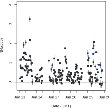
Figure 4 shows the hourly averages of measured NH₃from the LBNL laser spectrome-ter and the mean results from the 12 h samples collected by the DRI filspectrome-ter system. Both LBNL and DRI data show that NH3was generally between 0 and 2 ppb, with a few pe-5

riods of higher mixing ratios. Near 13 June, a synoptic event introduced cooler air from the north with lower temperatures and mild precipitation, reducing NH3 concen-trations significantly. The averages of the LBNL measurements were lower than the filter samples on 24 June, and similar to or higher than the filter samples on 25 June (see Table 2). Inspection of the LBNL data suggests that a significant fraction of the 10

data was noisy and did not pass quality control criteria (∼50% in some of the 12 h peri-ods), perhaps causing the poor correlation between LBNL averages and the DRI filter measurements.

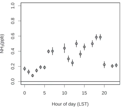
We also examined the diurnal variations in NH3. As shown in Fig. 5, there was a significant diurnal cycle with lower mixing ratios at night and higher mixing ratios 15

during the day. This is consistent with having predominantly downslope winds carrying NH3 free air from the Sierra Nevada during the night and upslope winds carrying air with NH₃from the Central Valley during the day (Dillon et al. 2002).

3.2 Calculated aerosol – gas equilibrium

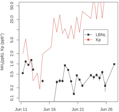
We considered whether the low NH3mixing ratios might limit ammonium-based aerosol 20

concentrations by comparing measured NH3with previously measured HNO3and the aerosol-gas equilibrium coefficient, Kp, which defines the minimum NH3*HNO3 prod-uct required to form NH4NO3 aerosol (Stelson et al., 1982). Figure 6 shows that Kp

>>1 ppb2 for most of the observation period. Earlier work at Blodgett showed that HNO₃mixing ratios fell in a range of 0.3 to 1.5 ppb (5%−95%) for June–October (Mur-25

ACPD

Full Screen / Esc

Printer-friendly Version Interactive Discussion

EGU ratio required to support aerosol NH₃*HNO₃in equilibrium with gas phase constituents

is numerically equal to the value of Kp. Since the measured NH3mixing ratio is gener-ally significantly less than Kp, this suggests that aerosol NH3*HNO3will not be present in equilibrium with gases. We also note that although Kp was low during points earlier in June, there were also light rains, which would likely strip NH3, HNO3, and aerosols 5

from ambient air.

3.3 NH3Fluctuations, Fluxes, and Deposition Velocities

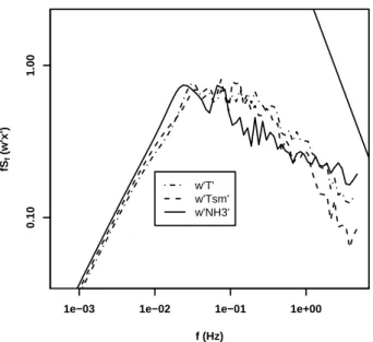
Before computing NH₃fluxes, we examined the power spectra for temporal variations in w’T’, w’T’sm, and w’NH3for each 1/2 h period over which NH3fluxes were calculated. By comparing the spectra of w’T’ and w’T’_sm, we can visually inspect the loss of high 10

frequency power in w’T’ introduced by smoothing T’ with the finite frequency response of the NH3 inlet system. A representative set of power spectra are shown in Fig. 7. As expected, the spectra for w’T’ and w’T’_smare similar, consistent with the smoothing reducing w’T’ by a small amount, and suggesting that NH₃ fluxes can be accurately recovered. We also note parenthetically that the high frequency slope of all three of 15

the spectra was not as steep as that expected for turbulence in a Komolgorov similarity theory, as observed by other researchers at this and other sites (Farmer et al., 2006).

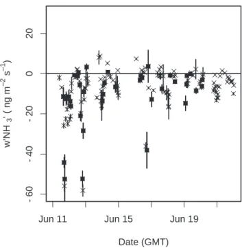
The NH₃fluxes calculated from the 10 Hz data are shown in Fig. 8. Most of the NH₃ fluxes were small (∼10 ng NH3m−2s−1) or negative. During a several day period early in the campaign when NH₃ mixing ratios were highest, large negative fluxes (−30 ng 20

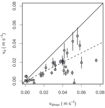
NH3 m−2 s−1) were observed, indicating that NH3 was being lost to the canopy by dry deposition. The mean flux during the measurement period was 9.2±1.1 ng NH3 m−2 _s−1_{. As a check of whether the estimated fluxes were realistic, we calculated} deposition velocities for a subset of the measured fluxes. The subset was obtained by requiring that the NH3 mixing was known to better than 50% (at 68% confidence). 25

As shown in Fig. 9, the measured deposition velocities are all less than the maximum deposition velocity estimated from the measured turbulence conditions using Eq. (8),

ACPD

Full Screen / Esc

Printer-friendly Version Interactive Discussion

EGU with a typical ratio for the measured to maximum deposition velocity of approximately

0.5. This is consistent with some combination of imperfect sticking to leaf surfaces and stomatal resistance to NH3uptake by the leaves.

3.4 Transport model estimates of NH₃concentrations

The map of the estimated surface NH₃fluxes from cattle is shown in Fig. 10. Surface 5

fluxes range over several orders of magnitude, reflecting the strong emissions from the Central Valley and low emissions from the mountainous regions of the Sierra Nevada. Figure 10 includes an example ensemble of 12-h particle back-trajectories representing a measurement at BFRS at 13:00 h local time on 12 June 2006. This example shows that some particle tracks sweep backward into the Central Valley where they come into 10

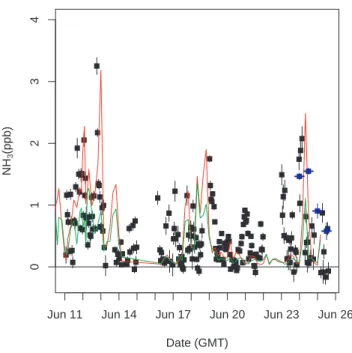
contact with high surface NH3fluxes. The predicted NH3concentrations from the back trajectory simulations are compared with measured NH₃ in Fig. 11. Measured NH₃ is generally a factor of ∼2 higher than NH3 predicted with deposition and a factor of ∼2 less than NH3 predicted without deposition. The temporal variations in predicted and measured NH₃ mixing ratios match reasonably well. This is likely because the 15

large variations are caused by variations in the amount of air reaching BFRS from areas in the Central Valley where NH3fluxes are highest.

4 Conclusions

We performed an exploratory study of NH3mixing ratios and fluxes at Blodgett Forest during June, 2006. The 1 h averaged NH3 mixing ratios ranged from non-detection 20

(<0.2 ppb) to about 2 ppb, typical of a low-background site removed from significant

sources. The diurnal variations were consistent with upslope flows bringing air with higher NH3to the site during the day. The observed NH3 mixing ratios were not suffi-cient to support NH₄NO₃ aerosol in equilibrium with gas phase NH₃assuming HNO₃ was similar to that observed at the site previously. NH3 fluxes, measured using the 25

ACPD

Full Screen / Esc

Printer-friendly Version Interactive Discussion

EGU eddy covariance method, were generally small or negative, consistent dry deposition

to the vegetation and no significant net emission. Calculated deposition velocities were generally about half of the maximum expected for deposition to a canopy with aerody-namic and leaf boundary layer resistance but no resistance to leaf uptake (perfect stick-ing to leaves). This is not surprisstick-ing given the nitrogen poor soils in the Sierra foothills. 5

Last, we predicted NH3 at BFRS by combining a simple NH3 emission inventory that considered only emissions from cows (dairy and meat) with a particle back-trajectory model. Measured and predicted NH₃concentrations showed substantially similar tem-poral patterns over synoptic time periods. Predictions with and without NH3deposition bracketed the measured NH3mixing ratios. On the basis of these measurements, we 10

conclude that NH₃ from the Central Valley had a small but measurable effect on NH3 mixing ratios at the BFRS site during the short period of this study, but further mea-surements would be necessary to determine the whether the same patterns prevail over longer periods, particularly between different seasons.

Acknowledgements. We acknowledge B. Duncan, D. Dibartolomeo, and J. Hatch for assistance

15

in construction of the instrument packaging and thermal control systems, M. Zahniser and D. Nelson for technical advice on the use of the NH₃ spectrometer. A. Goldstein generously shared the research infrastructure at BFRS, while D. and S. Rambeau provided invaluable assistance with arrangements for field work at BFRS. S. Kohl of the Desert Research Institute prepared the filter sampler and performed the analysis of the integrated NH₃mixing ratios. J. Lin

20

generously provided the STILT model for the atmospheric transport simulations. The NOAA Air Resources Laboratory (ARL) provided the assimilated meteorology used to drive STILT. N. Brown, R. Cohen, D. Farmer, M. Gallagher, A. Lashgari, M. Lunden and T. Ryerson provided valuable advice and discussion. This work was supported by the California Air Resources Board and by the Laboratory Directors Research and Development Program at the Lawrence

25

Berkeley National Laboratory.

ACPD

Full Screen / Esc

Printer-friendly Version Interactive Discussion

EGU

References

Baldocchi, D. D., Hicks, B. B. and Meyers, T. P.: Measuring Biosphere-Atmosphere Exchanges of Biologically Related Gases with Micrometeorological Methods, Ecology (Tempe) 69(5), 1331–1340, 1988.

Battye, W., Aneja, V. P., and Roelle, P. A.: Evaluation and improvement of ammonia emissions

5

inventories, Atmos. Environ., 37(27), 3873–3883, 2003.

Chow, J. C., Chen, L. W. A., Watson, J. G., Lowenthal, D. H., Magliano, K. A. Turkiewicz, K. and Lehrman, D. E.: PM2.5 chemical composition and spatiotemporal variability during the California Regional PM10/PM2.5 Air Quality Study (CRPAQS), J. Geophys. Res.-Atmos., 111(D10), 2006.

10

Chow, J. C., Watson, J. G., Bowen, J. L., Frazier, C. A., Gertler, A. W., Fung, K. K., Landis, D., and Ashbaugh, L. L.: A sampling system for reactive species in the western United States, Sampling and Analysis of Airborne Pollutants, Ed. E. D. Winegar and L. H. Keith, New York, Lewis, 209–228, 1993.

Dillon, M. B., Lamanna, M. S., Schade, G. W., Goldstein, A. H., and Cohen, R. C. Chemical

15

evolution of the Sacramento urban plume: Transport and oxidation, J. Geophys. Res.-Atmos., 107(D5–D6), 4045, 2002.

Draxler, R. R. and Hess, G. D.: An overview of the HYSPLIT 4 modeling system for trajectories, dispersion, and deposition, Aust. Meteorol. Mag., 47, 295–308, 1998.

Farmer, D. K., Wooldridge, P. J., and Cohen, R. C.: Application of thermal-dissociation laser

20

induced fluorescence (TD-LIF) to measurement of HNO3, Sigma alkyl nitrates, Sigma peroxy nitrates, and NO₂fluxes using eddy covariance, Atmos. Chem. Phys, 6, 3471–3486, 2006. Fischer, M. L., Littlejohn, D., Lunden, M. M., and Brown, N. J.: Automated measurements of

ammonia and nitric acid in indoor and outdoor air, Environmental Science & Technology, 37(10), 2114–2119, 2003.

25

Foken, T. and Wichura, B.: Tools for quality assessment of surface-based flux measurements, Agr. Forest. Meteorol., 78(1–2), 83–105, 1996.

Goldstein, A. H., Hultman, N. E., Fracheboud, J. M., Bauer, M. R., Panek, J. A., Xu, M., Qi, Y., Guenther, A. B., and Baugh, W.: Effects of climate variability on the carbon dioxide, water, and sensible heat fluxes above a ponderosa pine plantation in the Sierra Nevada

30

(CA), Agricultural & Forest Meteorology ,101(2–3), 113–129, 2000.

ACPD

Full Screen / Esc

Printer-friendly Version Interactive Discussion

EGU

of nitrogen oxides over a temperate deciduous forest, J. Geophys. Res.-Atmos., 109(D8), 2004.

Kirchstetter, T. W., Maser, C. R. and Brown, N. J.: Ammonia emisson inventory for the state of Wyoming, Berkeley, CA, E.O. Lawrence Berkeley National Laboratory, 2002.

Kurpius, M. R., McKay, M., and Goldstein, A. H.: Annual ozone deposition to a Sierra Nevada

5

ponderosa pine plantation, Atmos. Environ., 36(28), 4503–4515, 2002.

Lin, J. C., Gerbig, C., Wofsy, S. C., Andrews, A. E., Daube, B. C., and Grainger, B. B. S. C. A., Bakwin, P. S., and Hollinger, D. Y.: Measuring Fluxes of Trace Gases at Regional Scales by Lagrangian Observations: Application to the CO2 Budget and Rectification Airborne (CO-BRA), Study. J. Geophys. Res. 109, doi:10.1029/2004JD004754, 2004.

10

Lin, J. C., Gerbig, C., Wofsy, S. C., Andrews, A. E., Daube, B. C., Davis, K. J., and Grainger, C. A.: A near-field tool for simulating the upstream influence of atmospheric observations: The Stochastic Time-Inverted Lagrangian Transport (STILT) model - art. no. 4493, J. Geophys. Res.-Atmos., 108(D16), 4493, 2003.

Lunden, M. M., Revzan, K. L., Thatcher, M. L. F. L., Littlejohn, D., Hering, S. V., and Brown,

15

N. J.: The transformation of outdoor ammonium nitrate aerosols in the indoor environment, Atmos. Environ., 37, 5633–5644, 2003.

Malm, W. C., Pitchford, M. L., Scruggs, M., Sisler, J. F., Ames, R., Copeland, S., Gebhart, K. A., and Day, D. E.: Spatial and Seasonal Patterns and Temporal Variability of Haze and It’s Constituents in the United States, Fort Collins, Cooperative Institute for Research in the

20

Atmosphere, Colorado State University, 2000.

Murphy, J. G., Day, A., Cleary, P. A., Wooldridge, P. J., and Cohen, R. C.: Observations of the diurnal and seasonal trends in nitrogen oxides in the western Sierra Nevada, Atmos. Chem. Phys., 6, 5321–5338, 2006,http://www.atmos-chem-phys.net/6/5321/2006/.

NRC: Research priorities for airborne particulate matter. I. Immediate priorities and a

long-25

range research portfolio, Washington, DC, National Academy Press, 1998.

NRC: Research priorities for airborne particulate matter, III. Early Research Progress, Wash-ington, DC, National Academy Press, 2000.

Potter, C., Krauter, C., and Klooster, S.: Statewide Inventory Estimates Statewide Inventory Es-timates of Ammonia Emissions from of Ammonia Emissions from Native Soils and Chemical

30

Native Soils and Chemical Fertilizers in Fertilizers in California, Sacramento, California Air Resources Board, 2001.

Stelson, A. W. and Seinfeld, J. H.: Relative-Humidity and Temperature-Dependence of the

ACPD

Full Screen / Esc

Printer-friendly Version Interactive Discussion

EGU

Ammonium-Nitrate Dissociation-Constant, Atmos. Environ., 16(5), 983–992, 1982.

Tarnay, L., Gertler, A. W., Blank, R. R., and Taylor, G. E. Preliminary measurements of summer nitric acid and ammonia concentrations in the Lake Tahoe Basin air-shed: implications for dry deposition of atmospheric nitrogen, Environ. Pollut., 113(2), 145–153, 2001.

Wesely, M. L.: Parameterization of Surface Resistances to Gaseous Dry Deposition in

5

Regional-Scale Numerical-Models, Atmos. Environ., 23(6), 1293–1304, 1989.

Zahniser, M. S.: Urban Ammonia Source Characterization Using Infrared Quantum Cascade Laser Spectroscopy, National Atmospheric Deposition Program (NADP) Meeting, Potomac, MD, 2003.

Zhang, Q., Carroll, J. J., Dixon, A. J., and Anastasio, C.: Aircraft measurements of nitrogen

10

and phosphorus in and around the Lake Tahoe Basin: Implications for possible sources of atmospheric pollutants to Lake Tahoe, Environmental Science & Technology, 36(23), 4981– 4989, 2002.

ACPD

Full Screen / Esc

Printer-friendly Version Interactive Discussion

EGU Table 1. Cattle stocking, area, and estimated NH₃flux by county.

County Beef Cows Dairy Cows Other Cattle area (km2_{) Flux (ng NH} 3m−2s−1) Alameda 9401 6 10 405 1888 8 Alpine 1560 0 551 1891 1 Amador 10 112 20 9104 1518 9 Butte 8979 1261 9191 4197 4 Calaveras 14 390 222 12 878 2611 8 Colusa 0 0 7957 2946 2 Contra Costa 0 0 11 596 1843 5 Del Norte 1018 4703 4154 2580 5 El Dorado 4115 9 3551 4380 1 Fresno 23 422 90 550 282 547 15 265 28 Glenn 17 438 17 304 30 655 3366 22 Humboldt 22 333 16 732 24 041 9146 8 Imperial 0 0 386 634 10 687 27 Inyo 0 0 8278 26 120 0 Kern 36 779 74 708 148 553 20 841 14 Kings 5130 138 292 126 108 3561 111 Lake 4764 4 4378 3220 2 Lassen 25 381 38 23 905 11 667 3 Los Angeles 0 0 2092 10 396 0 Madera 15 723 48 086 82 972 5468 32 Marin 9105 10 309 15 998 1331 31 Mariposa 10 204 245 12 130 3715 5 Mendocino 0 0 7691 8983 1 Merced 29 534 223 303 212 270 4937 133 Modoc 41 564 14 33 615 10 097 6 Mono 2989 0 2938 7794 1 Monterey 25 430 1606 46 025 8504 7 Napa 4300 245 3453 1930 3 Nevada 3007 108 1927 2451 2 Orange 392 0 401 2021 0 Placer 0 0 10 004 3595 2 Plumas 5766 7 10 644 6537 2 Riverside 3670 90 359 87 042 18 451 14 Sacramento 16 392 18 337 32 807 2472 31 San Benito 14 408 935 24 054 3556 9 San Bernardino 2918 158 240 110 185 51 334 8 San Diego 6363 5729 13 709 10 752 3 San Francisco 0 0 0 120 0 San Joaquin 19 629 103 534 95 196 3582 86 San Luis Obispo 38 268 550 44 928 8459 7

San Mateo 1474 6 941 1150 2 Santa Barbara 19 482 2669 21 183 7007 5 Santa Clara 0 0 12 692 3304 3 Santa Cruz 984 176 2275 1140 2 Shasta 16 618 562 11 225 9690 2 Sierra 3339 0 3777 2441 2 Siskiyou 34 750 1518 28 421 16 094 3 Solano 14 560 3947 26 605 2123 18 Sonoma 14 311 31 986 35 301 4034 26 Stanislaus 42 007 162 878 221 060 3824 142 Sutter 0 0 5321 1543 3 Tehama 29 027 5489 33 679 7555 8 Trinity 2671 12 2252 8137 0 Tulare 31 171 412 462 456 491 12 349 101 Tuolumne 6855 108 5288 5723 2 Ventura 4357 17 4544 4724 1 Yolo 6773 2012 8124 2594 6 Yuba 7419 3325 20 694 1615 17 14157

ACPD

Full Screen / Esc

Printer-friendly Version Interactive Discussion

EGU Table 2. Comparison of NH₃mixing ratios (ppb) from DRI filter samples and averages.

Date time (GMT) Filter LBNL 24 Jun 2006 07:00 1.46 (0.05) 0.74 (0.28) 24 Jun 2006 19:00 1.55 (0.05) 0.36 (0.13) 25 Jun 2006 07:00 0.90 (0.12) 0.56 (0.32) 25 Jun 2006 19:00 0.58 (0.14) 0.91 (0.30)

ACPD

Full Screen / Esc

Printer-friendly Version Interactive Discussion

EGU Fig. 1. Satellite mosiac image showing the Blodgett Forest Research Station in the forested

western foothills of the central Sierra Nevada of California, and the mixed use (agricultural and urban) areas of the nearby Sacramento Valley area.

ACPD

Full Screen / Esc

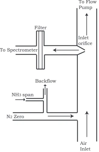
Printer-friendly Version Interactive Discussion EGU Backflow NH3 span N2 Zero Air Inlet Inlet orifice Filter To Spectrometer To Flow Pump

Fig. 2. Schematic illustration of the air sampling manifold with critical orifice flow inlet and air

filter. Automated instrument zero and span calibrations are performed by periodically flowing N₂into inlet, either without or with the addition of NH₃from a permeation tube source.

ACPD

Full Screen / Esc

Printer-friendly Version Interactive Discussion EGU - 10 0 10 20 30 0 5 10 15 Time (s) NH3 (ppb)

Fig. 3. Time series of NH₃mixing ratio showing transient decay following removal of NH₃span gas from zero air flow to instrument inlet.

ACPD

Full Screen / Esc

Printer-friendly Version Interactive Discussion EGU Date (GMT) NH 3 (ppb)

Jun 11 Jun 14 Jun 17 Jun 20 Jun 23 Jun 26

01234

Fig. 4. Hourly NH₃mixing ratios measured at Blodgett Forest in June, 2006. NH₃data from the laser-spectrometer (black symbols) are averaged into 12 h bins for comparison with integrating filter samples (blue symbols) collected with a sampling system provided by the Desert Research Institute.

ACPD

Full Screen / Esc

Printer-friendly Version Interactive Discussion EGU ● ● ● ● _{● ●} ● ● ● ● ● ● ● ● ● ● ● ● ● ● 0 5 10 15 20 0.0 0.2 0.4 0.6 0.8 1 .0 Hour of day (LST) NH 3 (ppb)

Fig. 5. Mean diurnal variation in surface NH₃mixing ratio from 11 to 26 June 2006.

ACPD

Full Screen / Esc

Printer-friendly Version Interactive Discussion EGU 0.1 0.2 0.5 1.0 2.0 5.0 20.0 50 .0 NH 3 (ppb), Kp (ppb 2 )

Jun 11 Jun 16 Jun 21 Jun 26

LBNL Kp

Fig. 6. Comparison of NH₃mixing ratio (black) and aerosol-gas equilibrium partitioning coeffi-cient, Kp (red), indicating minimum product of gas phase NH₃and HNO₃mixing ratios neces-sary for NH₄NO₃aerosol to be found in equilibrium with gas phase constituents.

ACPD

Full Screen / Esc

Printer-friendly Version Interactive Discussion EGU f (Hz) fS f (w'x')

1e−03 1e−02 1e−01 1e+00

0.10

1.00

w'T' w'Tsm' w'NH3'

Fig. 7. Power spectra of covariance in vertical wind speed with sonic temperature, w’T’,

smoothed sonic temperature, w’T’_sm, and fluctuations in NH₃mixing ratio, w’NH₃’. The straight line in upper right shows −4/3 slope expected for fluctuation spectra in an inertial sublayer.

ACPD

Full Screen / Esc

Printer-friendly Version Interactive Discussion EGU -6 0 -4 0 -2 0 0 2 0 Date (GMT) w'NH 3 ' ( ng m −− 2 s −− 1 )

Jun 11 Jun 15 Jun 19

Fig. 8. Eddy covariance measurement of NH₃ flux for all time points (crosses) and for those passing quality control criteria for use in calculating deposition velocities (filled squares).

ACPD

Full Screen / Esc

Printer-friendly Version Interactive Discussion EGU ● ● ● ● ● ● ● ● ● ● ● ● ● ● ● ● ● ● ● ● ● ● ● ● ● ● ● ● ● ● ● ● ● ● ● 0.00 0.02 0.04 0.06 0.08 0.00 0.02 0.04 0.06 0.0 8 vdmax ( m s−− 1 ) vd ( m s −− 1 )

Fig. 9. Scatter plot comparison of measured deposition velocity, v_d, and maximum deposition velocity in the case that all molecules reaching the leaf surface are absorbed, v_dmax.

ACPD

Full Screen / Esc

Printer-friendly Version Interactive Discussion

EGU Fig. 10. Map of California showing estimated NH₃emissions (ng NH₃m−2_s−1_{) and an example}

12 h back trajectory calculation of showing particles converging at BFRS at midday on 12 June 2006.

ACPD

Full Screen / Esc

Printer-friendly Version Interactive Discussion EGU Date (GMT) NH 3 (ppb)

Jun 11 Jun 14 Jun 17 Jun 20 Jun 23 Jun 26

01234

Fig. 11. Measured hourly NH₃mixing ratios from LBNL system (black points), DRI 12 h inte-grated sampler results (blue points), and predicted NH₃ mixing ratios predicted from the back trajectory calculations and cattle-only NH₃emission inventory. Predicted NH₃is scaled to fit on plot so that NH₃ predicted without deposition (red line) is scaled by a factor of 0.5, while NH₃ predicted with deposition (green line) is scaled by a factor of 2.