Regional pollution potentials of megacities and other major population centers

(1)

HAL Id: hal-00302377

https://hal.archives-ouvertes.fr/hal-00302377

Submitted on 19 Dec 2006

HAL is a multi-disciplinary open access

archive for the deposit and dissemination of sci-entific research documents, whether they are pub-lished or not. The documents may come from teaching and research institutions in France or abroad, or from public or private research centers.

L’archive ouverte pluridisciplinaire HAL, est destinée au dépôt et à la diffusion de documents scientifiques de niveau recherche, publiés ou non, émanant des établissements d’enseignement et de recherche français ou étrangers, des laboratoires publics ou privés.

Regional pollution potentials of megacities and other

major population centers

M. G. Lawrence, T. M. Butler, J. Steinkamp, B. R. Gurjar, J. Lelieveld

To cite this version:

M. G. Lawrence, T. M. Butler, J. Steinkamp, B. R. Gurjar, J. Lelieveld. Regional pollution potentials of megacities and other major population centers. Atmospheric Chemistry and Physics Discussions, European Geosciences Union, 2006, 6 (6), pp.13323-13366. �hal-00302377�

(2)

ACPD

6, 13323–13366, 2006 Regional pollution potentials of major population centers M. G. Lawrence et al. Title Page Abstract Introduction Conclusions References Tables Figures ◭ ◮ ◭ ◮ Back Close

Full Screen / Esc

Printer-friendly Version Interactive Discussion

EGU Atmos. Chem. Phys. Discuss., 6, 13323–13366, 2006

www.atmos-chem-phys-discuss.net/6/13323/2006/ © Author(s) 2006. This work is licensed

under a Creative Commons License.

Atmospheric Chemistry and Physics Discussions

Regional pollution potentials of

megacities and other major population

centers

M. G. Lawrence1, T. M. Butler1, J. Steinkamp1, B. R. Gurjar2, and J. Lelieveld1

1

Max-Planck-Institut f ¨ur Chemie, Postfach 3060, 55020 Mainz, Germany

2

Indian Institute of Technology (IIT) – Roorkee, Department of Civil Engineering, Roorkee 247667, India

Received: 1 December 2006 – Accepted: 5 December 2006 – Published: 19 December 2006 Correspondence to: M. G. Lawrence (lawrence@mpch-mainz.mpg.de)

(3)

ACPD

Full Screen / Esc

Abstract

Megacities and other major population centers represent important, concentrated sources of anthropogenic pollutants to the atmosphere, with consequences for both local air quality and for regional and global atmospheric chemistry. The tradeoff be-tween the regional buildup of pollutants near their sources versus long-range export 5

depends on meteorological characteristics which vary as a function of geographical location and season. Both horizontal and vertical transport contribute to pollutant ex-port, and the overall degree of export is strongly governed by the chemical lifetimes of pollutants. We provide a first quantification of this tradeoff and the main factors in-fluencing it in terms of “regional pollution potentials”, metrics based on simulations of 10

artificial, representative tracers using the 3-D global model MATCH (Model of Atmo-spheric Transport and Chemistry). The tracers have three different lifetimes (1, 10, and 100 days) and are emitted from 36 continental point sources representing the 30 cur-rent largest cities around the world plus 6 additional major population centers. Several key features of the export characteristics emerge: 1) long-range near-surface pollu-15

tant export is generally strongest in the middle and high latitudes, especially for source locations in Eurasia; 2) on the other hand, pollutant export to the upper troposphere is greatest in the tropics, due to transport by deep convection; 3) not only are there order of magnitude interregional differences, such as between low and high latitudes, but also often substantial intraregional differences, for instance between the sources in 20

western India and Pakistan versus eastern India and Bangladesh; 4) contrary to what one might initially expect, efficient long-range export does not necessarily correspond with a more significant dilution of pollutants near their source, rather the amount of low-level, long-range export (e.g., below 1 km and beyond 1000 km) is well-correlated with exceedences of surface density thresholds on regional scales near the source (e.g., 25

within ∼1000 km), implying that pollutant buildup to high densities in the surface layer of the region surrounding the source location is more strongly influenced by vertical than horizontal transport.

(4)

ACPD

Full Screen / Esc

EGU

1 Introduction

For the past few thousand years, human populations have been clustering in increas-ingly large settlements. At present, there are about 20 cities worldwide with a popula-tion of ten million or greater (see Table1), and 30 with a population of about 7 million or greater, and these numbers are expected to grow considerably in the near future. This 5

confluence of human activity in so-called “megacities” (e.g.,Molina and Molina,2004) leads to serious issues in municipal management, such as the coordination of public and private transport, fluid and solid waste disposal, and local air pollution. The latter is known to have significant consequences for human health and regional crop production (e.g.,Chameides et al.,1994;Emberson et al.,2001). On the other hand, emissions 10

of longer-lived pollutants from these concentrated population centers can affect atmo-spheric chemistry on the continental and global scale. The balance between local and long-range effects can be anticipated to depend strongly on regional meteorological and geographical differences. Here we address the question: What are the common features and differences in the regional and long-range dispersion characteristics for 15

air pollutants emitted from large, concentrated urban sources?

We examine this issue using artificial, representative tracers in a global 3-D chemistry-transport model (CTM). The tracers are emitted from 36 continental sur-face layer point sources, which represent the 30 most populated cities worldwide in 2000, plus six selected additional major population centers, which particularly help to 20

improve the global coverage of the analysis. Three tracers are released from each source location, with exponential decay lifetimes of 1, 10, and 100 days. These can be applied generically to understanding the anticipated typical outflow characteristics of a wide range of trace gases and aerosols. For instance, the typical lifetime of aerosols (sulfate, organic and elemental carbon, nitrate, etc.) generally lies between 1 and 25

10 days, and the global mean lifetimes of several key reactive trace gases fall in this range, including O3(∼25 d), CO (∼60 d), NOx(∼2 d), ethane (∼100 d), propane (∼30 d) and butane (∼3 d). The results of this study are complementary to those in Butler et

(5)

ACPD

Full Screen / Esc

al. (2006a)1, in which we examine the effect of megacity emissions more specifically on global and regional O3 chemistry, based on the megacity emissions work of Gur-jar et al. (2004), Gurjar and Lelieveld (2005), and Butler et al. (2006b)2. The generic tracer approach used here allows these results to also be applicable to other classes of airborne pollutants, such as Hg, Pb, and persistent organic pollutants (POPs). 5

The mean geographical distributions of these tracers are compared making use of a set of metrics which helps quantify either the degree of export or the coherent retention of the tracers in the source region. Both horizontal and vertical transport contribute to tracer outflow. Horizontal dispersion in the boundary layer (BL) transports pollutants to other regions, where they can still have direct effects on health, agriculture, and visibil-10

ity. Vertical dispersion, especially by cumulus convection, removes pollutants from the surface layer, but in turn transports them to the free and upper troposphere, where the lifetimes of many real trace gases and aerosols are much longer, their climate effects (e.g., influence on cirrus properties and as greenhouse gases) are more significant, and the potential exists for further transport into the stratosphere. It is not clear a priori 15

what the relative quantitative roles of horizontal and vertical transport are, and how this might vary on a regional basis; this is examined here in light of the regional pollution potential metrics.

We have chosen to use a global model so that we can make a comparative analysis of the outflow characteristics of the full large set of chosen source locations. Our focus 20

is on the outflow and pollutant distribution on regional, continental and global scales. The alternative of using a regional model would allow a more detailed analysis of lo-cal meteorology and regional pollutant distribution, and has provided valuable insights

1

Butler, T. M., Lawrence, M. G., Gurjar, B. R., and Lelieveld, J.: The effects of emissions from megacities on global ozone chemistry, Atmos. Chem. Phys. Discuss., in preparation, 2006a.

2

Butler, T. M., Lawrence, M. G., Gurjar, B. R., van Aardenne, J., Schultz, M., and Lelieveld, J.: The representation of emissions from megacities in global emissions inventories, Atmos. Environ., submitted, 2006b.

(6)

ACPD

Full Screen / Esc

EGU through detailed studies of individual cities (e.g.,Guttikunda et al.,2005;de Foy et al.,

2006), though it would be prohibitive to set up as many comparable simulations as would be needed to address the question posed here. We also have limited our dis-cussion to the most significant points; in addition, an electronic supplement is included with a full set of figures for the individual source locations, on an annual and seasonal 5

mean basis, as well as key tables and figures for tracers with different lifetimes.

In the following section we provide descriptions of the choice of source locations and tracers, the metrics considered in this study, and the global model MATCH-MPIC used for the simulations. Following that, we discuss the qualitative and quantitative dispersion characteristics for the set of tracers, focusing on three particular issues: low-10

level long-range export, vertical transport to the upper troposphere (UT), and regional exceedences of density thresholds. Our key conclusions are summarized in the final section, along with recommendations for future studies.

2 Methods

2.1 Tracer source locations 15

Table1lists the chosen major population center (MPC) tracer source locations for the simulations, along with the approximate population of each, and the corresponding model latitude and longitude. Thirty of these MPCs correspond to the worldwide most populated cities in 2000, with populations ranging from about 7 million (Hong Kong, Teheran and Chicago) to more than 20 million (Mexico City and Tokyo). In addition, 20

six additional major population centers are included (Po Valley, Italy; Johannesburg, South Africa; Szechuan Basin, China; Sydney, Australia; Atlanta, USA; and Bogota, Colombia), which have been chosen particularly to improve the global coverage of the source location dataset used in this study. Some other source locations are also to an extent representative of even greater metropolitan areas, such as the Pearl River Delta 25

(7)

ACPD

Full Screen / Esc

extended metropolis surrounding New York City. Note that we actually included about ten other source locations in our simulations, some with much smaller populations, but determined that they did not provide any additional major information beyond the conclusions that are drawn based on the selected set; in a few cases some of these additional tracer results will be referred to below to emphasize certain points. Through-5

out this study we will refer to the selected set of megacities and other large population centers collectively as “major population centers”, or “MPCs”.

The geographical distribution of the locations of these MPCs can be seen in Fig.1, which is discussed in more detail in Sect.3. Considering first the “proper” megacities, most are in the northern hemisphere, and the greatest concentration of megacities 10

is clearly in Asia, though there is a relatively good global coverage. The coverage is improved considerably with the inclusion of the additional MPCs mentioned above, especially Johannesburg and Sydney. The majority of the MPCs are either directly coastal, or within about 100 km of a coast (mostly oceanic, though in some cases like the Po Valley, Teheran and Chicago, also near large seas and lakes). Because of this, 15

many of the MPCs are either nearly at sea level or are within a few hundred meters altitude. However, there are several exceptions to this, with a few being at very high el-evations, as listed in Table2. In general, the model at the resolution employed (T63) is able to capture the characteristic high elevation of these cities, especially for plateaus like the highveld around Johannesburg, although it often tends to underestimate due to 20

the smearing out of detailed orographic features in the model grid cells. One interesting exception to this is Lima, for which the geopotential altitude of the corresponding model grid is much higher than the actual altitude of the city. This is due to its close proxim-ity to the Andes mountain range, which is partially included in the grid cell including Lima. A few other MPCs are also affected by this interpolation of orography, especially 25

for mountains near coasts or valleys, though not as severely as Lima; the main MPCs affected are the Po Valley (modeled altitude: 942 m; actual elevation: ∼100−200 m), the Szechuan Basin (764 m vs. ∼200−500 m), Beijing (740 m vs. ∼40 m), and Rio de Janeiro (600 m vs. ∼10 m; note the proximity to Sao Paulo, which is at a much higher

(8)

ACPD

Full Screen / Esc

EGU altitude, as listed in Table2). For these MPCs, it can be expected that the results

pre-sented here will be biased towards more long-range transport in the free troposphere and less retention at low altitudes, as discussed for a few cases below. The deviations in modeled geopotential altitude for the remaining MPCs, at elevations near sea level, are generally small.

5

A set of artificial tracers is emitted at the same rate, 1 kg/s, from the model surface layer at each MPC source location. Following emission, the tracers are transported with the model parameterizations (described below), and a uniform global decay rate is applied to the tracer mixing ratios each time step. Three characteristic decay rates have been chosen: 1 d, 10 d, and 100 d, which correspond to the main range of tracers 10

of interest in urban and regional air pollution, as discussed in the introduction. The tracer mixing ratios were archived on a monthly mean basis.

2.2 Metrics

The metrics which are employed to examine the tracer distributions are focused on addressing two main questions:

15

– How much of the tracer mass is exported beyond a given distance (horizontal

and/or vertical)?

– How large is the geographical area surrounding the source location with a

sub-stantial pollution buildup?

We have examined a wide variety of metrics for quantifying the dispersion of these 20

tracers. In this paper, we focus on a subset of these, summarized in Table 3, which illustrate the main findings regarding global tracer dispersion characteristics. The first basic type of metric is the mass which is exported to a chosen minimum distance away from the city, in the horizontal and/or vertical. Here we will discuss total (column) and low-level (below 1 km) pollutant export over long ranges (“ELR”) in terms of the 25

(9)

ACPD

Full Screen / Esc

transported to more than 1000 km away from the source location; these are denoted as ELR_col and ELR_1km, respectively. We have also considered other distance thresholds (e.g., 500 km, 2000 km), but find the same qualitative results to hold as for 1000 km. Vertical transport to the upper troposphere (UT) is discussed mainly in terms of the fractional mass of each tracer which resides above 5 km, at any horizontal distance 5

from the source (EUT).

To compute ELRcol and ELR1km, it is necessary to determine the longi-tude/latitude coordinates of circles of the desired radii surrounding each cho-sen source point. We approximate such circles by determining the locations of a set of equidistant points around each source point. The transformation 10

from distances in meters to the graticule (latitude-longitude grid) is based on the radii of the WGS84 ellipsoid (National Imagery and Mapping Agency, http://earth-info.nga.mil/GandG/publications/tr8350.2/wgs84fin.pdf, 2000). Only the appropriate fraction of the tracer masses are taken for the set of grid cells which are on the bound-aries of the circles (i.e., partly inside and outside the circles); for these border grid cells, 15

the assumption is made that they are rectangular, and the fraction inside or outside the circle is calculated as an area weighted factor using the gridcell edges and the spline formed by the equidistant points (the error due to this assumption is<1%, which was tested by summing up the areas enclosed by the circles using this approach versus the actual analytically computed geometric surface area of the circles).

20

A completely different type of metric which we consider is the geographical area (including the source grid cell) in which the tracer density (in ng/m3) in the surface layer exceeds a chosen threshold. In Sect.3.4we consider three threshold densities, 1, 10, and 100 ng/m3, which we callA1,A10, andA100, respectively, although we fo-cus mainly on the results forA10. Note that we choose to work in density here, since 25

this is more commonly applied in air pollution studies (the conversion to mixing ratio at the surface is straightforward, since surface air has a density of close to 1 kg/m3). This metric is similar in principle to the “megacity footprint” defined byGuttikunda et al. (2005), in which they consider the area in which the emissions from a megacity

(10)

con-ACPD

Full Screen / Esc

EGU tribute to 10% or more of the monthly mean ambient concentrations of real pollutants

below 1 km altitude. The metricsA1,A10, andA100 as defined here give an indication of the coherence of the outflow plumes, that is, the extent to which they remain as con-centrated polluted regions (including, surrounding and downwind of the MPC) versus being rapidly dispersed and diluted to lower densities away from the source. We might 5

expect this metric to be to an extent orthogonal to ELR1kmandEUT, since they instead represent the transport and thus dilution of the tracer over large horizontal or vertical distances.

2.3 Model description

For this analysis we use the global 3-D Model of Atmospheric Transport and Chemistry 10

(MATCH). MATCH is a semi-offline model which has been described and evaluated in detail inRasch et al.(1997);Mahowald et al.(1997b,a);Lawrence et al.(1999,2003a); von Kuhlmann et al.(2003);Lang and Lawrence(2005a,b). The model transport and physics parameterizations are mostly based on the CCM3 (Kiehl et al.,1996). MATCH has been used to study a variety of topics, including long range transport of pollution 15

plumes (Lawrence et al.,2003a), and transport by deep convection and its effects on global tropospheric O3 (Lawrence et al., 2003b; Lawrence and Rasch,2005). Here we are particularly interested in the quality of the simulated tracer transport, especially in pollutant outflow regions. Previous studies have shown this to be generally very good for CO, C3H8 and other pollution tracers, with correlation coefficients between 20

simulated and observed values often being in the 0.7–0.9 range, and with the main exception being in regions where the emissions are not well represented, for example, due to the use of climatological biomass burning emissions (Lawrence et al.,2003a; Gros et al.,2003,2004;Salisbury et al.,2003).

The simulations discussed here are driven by data from the NCEP/NCAR reanalysis 25

project (Kalnay et al.,1996) at a horizontal resolution of T63 (96×192 grid points, or about 1.9◦), with 28 vertical levels from the surface to about 2 hPa. The setup is similar to that used in Lawrence et al.(1999) and von Kuhlmann et al. (2003), but focusing

(11)

ACPD

Full Screen / Esc

only on artificial tracers, and including the new plume ensemble tracer transport repre-sentation for deep convection fromLawrence and Rasch(2005). The model is run in a “semi-offline” mode, relying only on a limited set of input data fields, which are: surface pressure, geopotential, temperature, horizontal winds, surface latent and sensible heat fluxes, and zonal and meridional wind stresses. These are interpolated in time to the 5

model time step of 30 min, and used to diagnose transport by advection, vertical diffu-sion, and deep convection, as well as the tropospheric hydrological cycle (water vapor transport, cloud condensate formation and precipitation). All runs analyzed here were performed for the year 1995, which was chosen as a “neutral” year with regards to the ENSO. For the 1 and 10-day lifetime tracers, a 1-month spinup was provided, while for 10

the 100-day lifetime tracers a 1-year spinup period was used.

3 Qualitative and quantitative dispersion characteristics

In assessing the tracer dispersion characteristics, we focus on dispersion over hori-zontal scales of the order of 1000 km, which represents a rough boundary between regional and continental scale pollution. This scale should be appropriate for studies 15

with the model at T63 resolution, since a circle with a radius of 1000 km is represented by ∼100 model grid cells.

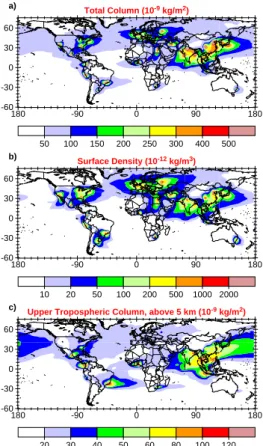
Figure 1 shows the annual mean column-integrated density summed over all of the τ=10 d tracers from the source locations listed in Table 1, along with the surface mixing ratio and the upper tropospheric column den-20

sity. The global outflow figures for the τ=1 d and τ=100 d tracers (see the electronic supplement http://www.atmos-chem-phys-discuss.net/6/13323/2006/ acpd-6-13323-2006-supplement.pdf) are qualitatively similar to the _{τ=10 d tracers,} though with less or more effective dispersion, respectively, as could be anticipated from the different lifetimes. In the following sections, we discuss the results based on 25

(12)

ACPD

Full Screen / Esc

EGU 3.1 Overall horizontal dispersion characteristics

An impression of the overall degree of dispersion of the tracers into the regions sur-rounding their source locations in terms of the column densities can be gained from Fig. 1a. For the τ=10 d tracers, the vast majority of the mass, generally exceeding about 95%, is exported out of the model column in which the source is located; even 5

for the_{τ=1 d tracers, more than about 60% of the mass is found outside of the source} column. However, export at this scale is not well resolved by the model, and it is more sensible to focus on quantifying the export to larger distances (e.g.,>1000 km), which can be done using ELR_col. Interestingly, we find that this metric does not vary consid-erably across all the source locations, only ranging from 62% to 84%, with typically a 10

small seasonal variability (standard deviation of the 12 monthly values of about 5%). Given that there is only a ∼30% relative difference between the minimum and maxi-mum values for ELRcol, this is not a particularly good metric for separating the regional characteristics, and thus is not listed in Table 4. For really differentiating horizontal export characteristics, we find that it is important to add a vertical component to the 15

metric, as discussed in the next section. 3.2 Low-level long-range export

The outflow in the model surface layer (Fig.1b) can be compared to the column den-sities (Fig. 1a), showing that the retention of pollutants near the surface tends to be stronger in the mid- and high-latitudes than in the tropics. For most sources, the sur-20

face flow pattern dominates the total (column) outflow pattern; the main exceptions to this are in the tropics, particularly in South America, where much of the mass is lofted to the UT, and the UT flow direction is different than near the surface.

In this section, we focus on the results for ELR1kmfor theτ=10 d tracers, which are listed in Table4. Overall, ELR1kmvaries by more than an order of magnitude, from 34% 25

for Moscow to 3.2% for Jakarta, with an average value of 14.1%, which makes this a good metric for distinguishing the MPCs in different regions. The greatest long-range

(13)

ACPD

Full Screen / Esc

export of pollutant mass near the surface is for the seven source locations in the region of approximately 0◦–50◦E and 25◦–55◦N (western Asia, Europe, and northern Africa), with an average ELR1km of 23.4% and an average rank of 5.1. These are followed by the NE Chinese cities (mean ELR1km=18.4%, mean rank of 9.3), and by the two northeastern USA source locations (mean ELR_{1km=17.7%, mean rank of 11.5). On} 5

the other end, the lowest values of ELR1kmfor theτ=10 d tracers are computed for the SE Asian cities, plus the Szechuan Basin, Mexico City, the South American cities Bo-gota, Sao Paulo, and Rio de Janeiro, and the African cities Lagos and Johannesburg, with a mean for these of ELR1km=5.6% and a mean rank of 31.5. As seen in Table2, several of these MPCs are at high elevations, so that a reduced ELR1kmfrom horizontal 10

transport to surrounding, lower-elevation regions could in part be expected. An addi-tional factor, deep convective transport, which influences ELR1kmat these locations, is discussed in the next section.

Seasonally, the low-level long-range export is almost uniformly largest during the win-ter. Since most of the MPCs are in the NH, this is reflected in the monthly mean values 15

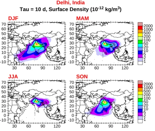
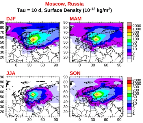
of ELR1km, which are highest during the northern hemisphere (NH) winter, ranging from 9.2% in August up to 16.9% in January. The most pronounced seasonality is simulated for the southern and eastern Asian cities, which are affected by the seasonal reversal of the monsoon winds and associated changes in deep convection. An example of this is shown in Fig.2 for Delhi. The electronic supplement shows that for MPCs in most 20

other regions, the main geographical dispersion patterns tend to be similar throughout the year, with a few exceptions. One of the strongest exceptions is Moscow (Fig.3), which has a pronounced outflow into the Arctic during the winter and spring, but pri-marily towards the south during summer. Istanbul, about 15◦S and 10◦W of Moscow, has a similar seasonal variability in the geographic patterns of the outflow, but much 25

less outflow reaching the far northern high latitudes. This contribution to the so-called “Arctic haze” is similar to what has been noted in previous studies (e.g.,Stohl et al., 2002), which have indicated that generally European pollution should contribute more strongly to the Arctic haze than North American or eastern Asian emissions. Here we

(14)

ACPD

Full Screen / Esc

EGU confirm this to be the case (see the electronic supplement for the full set of

compar-ative figures). However, we additionally find that the effectiveness of emissions from Moscow, on a per kg of emissions basis, in contributing to the Arctic haze is nearly an order of magnitude greater than that of emissions from Paris or London, and further-more that the seasonal variability of those two western European cities is much less 5

than that of Moscow.

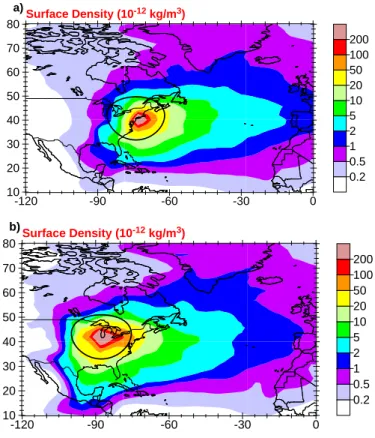
There are several other notable intra-regional differences in ELR1km, similar to those noted above for the seasonality of the Eurasian MPCs. In particular, New York has a rank of 16, versus nearby Chicago with a rank of 7 (we also examined additional tracers for Montreal and Toronto, which had ELR1km values very similar to Chicago). 10

This difference is depicted in Fig.4, which shows that the Chicago outflow is strong towards the south and the east, and to an extent also westwards, in contrast to the New York outflow, which is primarily towards the east over the Atlantic, where the tracers can be more readily lofted by warm conveyor belts along the U.S. east coast (Stohl,2001). Another notable difference is in southern Asia, where Delhi (rank 8) and Karachi (rank 15

12) are considerably more efficient low-level exporters than Mumbai (18), Kolkata (19) and Dhaka (20), mainly due to more efficient deep convective lofting of the outflow for the latter three, especially in the Asian summer monsoon, as discussed further in the next section. Further intraregional differences include Buenos Aires (17) and Lima (26) versus the rest of South America and Mexico City (30–35), and the Szechuan 20

Basin (31) versus the NE Chinese cities (6–13) and Seoul (15). We also noted that Melbourne, Australia, another of the additional tracers (not selected for Table4), has a value of ELR1km=20.0%, nearly twice that of Sydney (ELR1km=11.4%).

An additional important characteristic in terms of the impact of emissions on health and agriculture is how much of the long-range export remains over land, and how 25

much is over the oceans. New York and Chicago, discussed above (Fig.4), show a good example of this difference. Since most MPCs are near costs, the mean ELR1km limited to only land regions is 6.4%, slightly less than half of the mean ELR1km over both surfaces. The values and ranks of the individual tracers for outflow over land

(15)

ACPD

Full Screen / Esc

versus outflow over both land and sea are well correlated (the correlation between the rankings isr2=0.88, with a root mean square (rms) deviation of 3.6). Interestingly, this makes the distinction of MPCs at the extreme ends even stronger: for land-export only, the values of ELR1kmrange from 28.5% for Moscow (a land-locked city) down to 0.5% for Jakarta (on an island).

5

As noted in Sect.2.1, a few MPCs are at elevations in the model which are notably higher than their actual elevations (e.g., the Po Valley), which has the consequence that the ELR_1km values in Table 4 are likely to be lower limits for these MPCs. An interesting example of this is Eurasia, where the Po Valley, Istanbul, and Teheran lay nearly along a straight line from NW-SE, with about 1500−2000 km separating each. 10

The two MPCs at higher elevations (in the model), Po Valley and Teheran, have values for ELR1km of 18.5% and 17.2%, and ranks of 10 and 11, respectively, while Istanbul has a greater low-level export efficiency of ELR1km=21.7%, with a rank of 4. Besides elevation, one of the most important factors which influences the pollutant export is deep convection, as discussed in the following sections. Table4shows that the export 15

to the upper troposphere (EUT), which is indicative of deep convection, does not differ strongly for these MPCs (they are ranked 30–32). Though it is not possible to rule out that other factors may also have a strong influence on the ELR1km values for these MPCs (e.g., mean wind speeds), this comparison is at least suggestive that a lower elevation would tend to result in a moderate relative increase in ELR_1km for the Po 20

Valley of about 10–15%, to a value closer to that of Teheran. An interesting possibility for a future study in order to quantify the importance of this effect - and similarly of the effect of a substantial fraction of emissions being from elevated smoke-stacks for some MPCs – would be a follow-up set of sensitivity simulations with emissions from neighboring grid cells which are at different altitudes, along with emissions released 25

into different model layers besides the surface layer.

Finally, this section has focused so far only on the results for ELR1kmfor theτ=10 d tracers. We can also consider how the rankings for this general type of metric change if we make different choices for the outflow depth, minimum outflow distance, and tracer

(16)

ACPD

Full Screen / Esc

EGU lifetimes. For the outflow depth, we also examined the values for outflow restricted to

only the near-surface layer below 100 m, and find that this gives nearly identical rank-ings to the ELR1kmvalues listed here (r

2

=0.99, rms=1.0), though of course the values tend to be much smaller (on average 1.5%, close to the factor of 10 difference in the outflow volumes). For the dependence on the outflow distances, we can compare the 5

results for outflow beyond either 500 km or 2000 km, and find that again, the rankings compared to outflow beyond 1000 km do not change significantly (r2=0.98, rms=1.5, andr2=0.91, rms=3.2, respectively).

There are more notable differences for the rankings of the τ=1 d and τ=100 d tracers compared to theτ=10 d tracers (r2=0.55, rms=7.5, and r2=0.69, rms=6.1, respec-10

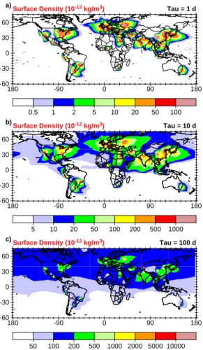
tively). To give a better indication of the overall similarity and differences in the outflow depending on the tracer lifetime, the surface layer outflow for the tracers with the three different lifetimes are plotted in Fig.5 with contour intervals which are scaled by the lifetimes (e.g., 10× larger for_{τ=10 d than for τ=1 d). The total global mass of each of} theτ=10 d tracers is 10× that of the τ=1 d tracers, though the τ=10 d tracers can be 15

expected to be more dispersed than theτ=1 d tracers (with the same applying to the relationship to the _{τ=100 d tracers). The degree of this enhanced dispersion for the} longer lifetime tracers can be clearly seen in Fig.5. While the τ=1 d tracers tend to remain relatively concentrated near their source locations, theτ=10 d tracers disperse readily over continental scales, though still show substantial peaks in the densities over 20

large regions near their sources. Much of the mass of theτ=100 d tracers, on the other hand, is spread out over the NH, in the lowest contour interval, and the peak mixing ratios at the sources are much less pronounced.

There are several cases where the tracers of one lifetime have a notably higher rank (more effective export beyond 1000 km) than the other two lifetime tracers from 25

the same MPC. In particular, relatively much more efficient export is computed for the τ=10 d tracers than for either the τ=1 d or τ=100 d from several cities, including Delhi, Mumbai, Kolkata, Karachi, Beijing, Tianjin, and Cairo. For Delhi, the most extreme case, the annual mean _{τ=10 d tracer has a rank of 8, while the τ=1 d and τ=100 d}

(17)

ACPD

Full Screen / Esc

tracers have ranks of 25 and 19, respectively. The reason for this is that the export from these MPCs tends to occur first in the BL (and in some cases in an overlying residual layer over the oceans), spreading over several thousand km before encoun-tering a region of strong mixing out of the BL, such as the intertropical convergence zone (ITCZ). This type of coherent outflow over the time-scale of about a week has 5

been studied in various field campaigns, in particular for the Asian winter monsoon during the Indian Ocean Experiment (INDOEX) (Lelieveld et al., 2001; Ramanathan et al.,2002), for which MATCH-MPIC was shown to accurately simulate the sharp tran-sition between polluted NH and cleaner SH surface-layer airmasses at the ITCZ on the three occasions when observations of this were made (Lawrence et al., 2003a). 10

For Hong Kong, on the other hand, the export is notably more efficient for the τ=1 d tracers (ranks 5, 22 and 29 forτ=1 d, 10 d, and 100 d, respectively), due to its closer proximity to the ITCZ, and the rapid BL export is only effective over a day or so; a similar behavior is also computed for Manila. At the other extreme, for the Po Valley theτ=100 d tracer is relatively far more effectively exported (ranks 22, 10 and 4); here, 15

the export distance for the shorter-lived tracers is limited by the basin geography, and regional meteorology characteristics (despite the overestimation of the elevation at this resolution), while the longer-lived pollution tends to be rather effectively retained in the surface layer of the surrounding regions over extended periods. Only a few other lo-cations show a tendency similar to the Po Valley, in particular Buenos Aires, Rio de 20

Janeiro, and Johannesburg, but considerably less pronounced. 3.3 Vertical export to the UT

Transport of certain pollutants from MPCs to the upper troposphere (UT) can be important for various global pollution and climate-related issues: for instance, cirrus clouds in the UT contribute significantly to the global long- and short-wave radiation 25

budget, and may be affected by the upwards transport of pollutants which influence the availability of ice nuclei (e.g.,Lohmann,2002); greenhouse gases such as O₃ are more efficient in the UT due to the colder temperatures (Lacis et al.,1990); the lifetimes

(18)

ACPD

Full Screen / Esc

EGU of many gases and aerosols tend to be much longer in the UT than near the surface;

and the UT serves as the gateway to the stratosphere, for instance for halogenated gases which can affect the stratospheric O3layer (WMO,2002). It is important to recall that the tracers considered here are all insoluble tracers; washout of soluble tracers will substantially reduce their transport to the UT. A rough rule of thumb (Crutzen and 5

Lawrence,2000) is that for soluble tracers with Henry’s Law coefficients of 103, 104, and 105M/atm, the transport to the UT will be about 15%, 50% and 85% as efficient, respectively, as the transport of an insoluble tracer. We plan a more detailed analysis of the fate of soluble tracers in a follow-up study.

Figure1c shows the column density above 5 km for all theτ=10 d MPC tracers, and 10

Table4lists the fractional masses of the MPC tracers which reside above 5 km (EUT). It is directly evident that the strongest export to the UT occurs for the tropical MPCs. This is mainly due to the greater intensity of deep convection in the tropics. There is a good correlation betweenEUT and the parameterized convective mass flux through 5 km altitude: for theτ=10 d tracers, we compute r2=0.63 for the correlation with the 15

convection in the source column, and r2=0.66 if instead the mean convective mass flux in the 500 km surrounding the source point is considered. For _{τ=1 d the} corre-lation improves tor2=0.81 (for the source column convection), while for the τ=100 d tracers it is much poorer (r2=0.32), as could be expected due to the less important role of episodic convective mixing for longer-lived tracers. There is also a relatively 20

strong anti-correlation betweenEUTand the absolute latitude of the MPCs (r 2

=0.63 for τ=10 d), although there are several clear outliers in both directions: on the high side, Sao Paulo, Rio de Janeiro, Tokyo, Osaka, Manila, and Bangkok; and on the low side, Delhi, Mumbai, Karachi, Lima, Teheran, and especially Cairo, for which only half as much makes it to the UT as would be expected from the linear regression, due to its 25

location in the downward branch of the Hadley Cell. On a regional basis, all but one of the last seven ranked MPCs is in Eurasia (the exception being Cairo), and the top five ranked MPCs for export to the UT are in southern Asia and Brazil.

(19)

convec-ACPD

Full Screen / Esc

tive activity, with values ranging from 9.6% for Moscow to 66.7% for Jakarta. It is worth noting that an even greater spread in the values would be expected for any trace gases or aerosols with lifetimes that increase with altitude, since this would result in a greater global mass for the tracers with more efficient export to the UT (whereas using the cur-rent setup provides a lower limit to the variability, since all tracers have the same global 5

total mass). For the τ=10 d tracers, there are 6 source locations with >50% of the tracer mass in the UT, with an average absolute latitude of 14◦. For shorter lifetimes, the variability is even greater, withEUTranging from 0.4–45.7% forτ=1 d tracer, while forτ=100 d tracer the range is reduced to 34.0–57.7%. Nevertheless, the ranks are generally similar (more so than for ELR1km), with correlations and deviations between 10

the rankings of the _{τ=1 d and τ=10 d tracers of r}2=0.88, rms=3.6, and between the τ=10 d and τ=100 d tracers of r2=0.72, rms=5.7.

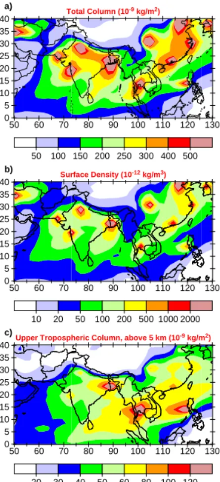
As in the previous section, it is also interesting here to consider the differences within sub-regions apparent in Fig.1. For the southern Asian MPCs, detailed in Fig. 6, the upwards transport of pollution is notably stronger from Kolkata and Dhaka (EUT=36.8– 15

39.2%) than from Karachi, Mumbai, and Delhi (22.5–27.6%), which are in the same latitude range but some 15–20◦ to the west, with the difference growing larger for the cities farther to the west, away from the highly convectively active Bay of Bengal region. Another notable intraregional difference is in South America, where the Brazilian MPCs and Bogota are much more efficient exporters to the UT (EUT=50.4–55.3%) than Lima 20

and Buenos Aires (26.5–31.2%). Also, the difference noted in the previous section between Sydney and Melbourne is seen here as well, with a factor of two difference between theEUTvalues of 34.5% and 17.2%, respectively.

Relating these results back to the previous section, the source to the UT also repre-sents a loss of tracer from the BL. Thus, one might expect that in regions where convec-25

tion is active, much of the tracer will have been transported out of the BL before it can be horizontally transported over long distances (e.g., beyond 1000 km), as was already alluded to in the previous section. This is supported by the strong anti-correlation (for theτ=10 d tracers) between EUTand ELR1km, withr

2

(20)

ACPD

Full Screen / Esc

EGU for the rankings. Thus, vertical transport by convection is a major factor in limiting

long-range low-level export. A remaining question is how this compares with the horizontal dilution of the tracers from the source grid cell scale (3–4×104km2) to regions extend-ing past 1000 km (order of 106km2). This is addressed from the practical standpoint of pollution impacts at the surface level in the next section.

5

3.4 Regional exceedences of density thresholds

The effects of pollutants on humans and agriculture depends on the amount of the pollutant present (in terms of either the density, concentration or mixing ratio), though the exact dependence differs for each pollutant, in terms of both the critical amounts and the exposure time-scales. In this section we examine a regional pollution poten-10

tial metric which indicates the anticipated degree of widespread exposure to elevated pollutant levels, above a chosen threshold density, in the outflow of each MPC.

An example of this metric,A10 (with a threshold density of 10 ng/m 3

), is given in Ta-ble4for the τ=10 d tracer. The values range over more than an order of magnitude, from 0.4−11.1 Mkm2, offering a good separation between the MPCs. The MPCs which 15

show the most extensive surface-layer pollution buildup around the source region in-clude those in Europe, western Asia, northern Africa, eastern China, and eastern North America. These are very similar to the regions for which ELR_1kmwas greatest; this sim-ilarity is discussed further below. A particularly interesting example of efficient regional pollution buildup is Delhi (rank 4). This is reminiscent of the so-called “Delhi fog” ( Gan-20

guly et al.,2006), a small-scale recurring buildup of pollution in the winter which can be so extreme that it results in shutdowns of airports and other facilities. Here, however, the pollution buildup is simulated over a much larger scale, and is primarily due to the coherent low-level outflow towards the southwest in the winter monsoon, as depicted in Fig.2. In December, Delhi has rank 2 forA10. In summer, on the other hand, when 25

the ITCZ over India causes effective lifting in the monsoon convection, Delhi actually becomes one of the least effective MPCs for regional pollution buildup, with a rank of 32. The least effective MPCs in the annual mean include those in Southeast Asia,

(21)

ACPD

Full Screen / Esc

Mexico City, the South American cities of Bogota, Rio de Janeiro and Sao Paulo, the central and southern African cities of Lagos and Johannesburg, and the Szechuan Basin in China, mainly regions where simulated deep convective lifting is particularly strong during significant parts of the year.

It may seem surprising that Mexico City, known to be a basin with substantial local 5

pollution buildup, would be one of the lowest-ranked amongst the tracers for A10. In order to examine whether this is a model artifact, or has a physical explanation, we can consider an additional metric, the fractional mass of the tracer which is retained in the lowest 1 km altitude within either the source cell itself or within a circle of a given radius surrounding the source (for which we considered 500 km, 1000 km and 10

2000 km). We did not generally include this metric in this study for two reasons: 1) for the larger radii, especially 2000 km, the rankings are generally similar to those forA10, since both are indicators of the retention of pollutants near the surface on regional to continental scales; and 2) the model can be expected to have difficulty resolving the smaller radii well, particularly the source grid cell itself. However, this metric can at 15

least be examined as a useful indicator in this particular case. In doing so, we find that Mexico City is amongst the source locations with the strongest retention in the source grid cell, with a rank of 5 in the annual mean. For retention within 500 km, however, it falls to rank 21. Thus, the model does simulate the strong local pollution buildup directly in the Mexico City basin, but ineffective buildup over the larger regional scales 20

that are considered withA10. Interestingly, some of the other source locations with the strongest simulated retention in the source grid cell are other well-known basins; in particular, Los Angeles is ranked first for this metric for all three lifetime tracers. We suspect the reason for this is that the NCEP/NCAR reanalysis winds are constrained by observations which include the tendency for local stagnation at these locations. 25

Nevertheless, it is clear that these features cannot be well resolved by the model, and for the rest of this section we focus only on the regional to continental scale surface-layer pollution buildup.

(22)

ACPD

Full Screen / Esc

EGU a function of the tracer lifetime, and the chosen threshold density. The importance of

tracer lifetime is seen in Fig.5, which shows the substantial difference in local pollution buildup versus long-range export due to the different lifetimes. Recall that the contours have been chosen to reflect the ratios between the total global masses of the tracers; if the tracers were distributed similarly, despite their different total masses, the figures 5

would look the same. The differences in the panels directly reflect the greater degree of dispersion of the longer-lived tracers. A key question, given these differences in dispersion, is whether or not the rankings tend to be similar for the various lifetimes. On the whole this is indeed the case, especially for the two longer-lived tracers; for example, for the metricA10 listed in Table 4, the correlations and deviations between 10

the rankings of the_{τ=1 d and τ=10 d tracers are r}2_{=0.67, rms=6.3, and between the} τ=10 d and τ=100 d tracers are r2=0.83, rms=4.3.

Since the choice of threshold density is rather arbitrary, it is interesting to consider a few simple calculations to illustrate the ranges which are sensible to focus on. At one extreme, if all the emissions of a givenτ=10 d tracer were to remain concentrated 15

only in the source cell, the resulting tracer density would be about 200−250 µg/m3. Of course, over a 10-day period, substantial dispersion occurs, so that only a small fraction of the tracer mass remains in the source cell, and the highest annual mean densities computed for any of the τ=10 d MPCs are actually around 4.8 µg/m3. In-terestingly, this does not change much for the other lifetimes; for_{τ=1 d, the maximum} 20

density is 3.3 µg/m3, and for τ=100 d, it is 4.5 µg/m3. Since the source rate is the same (1 kg/s) for all three lifetimes, this indicates that the mixing ratio near the source depends primarily on the dispersion rate, rather than on the lifetime of the tracer (that is, the modeled dispersion of air away from the source is occurring on time-scales of the order of a day or less). At the other extreme, if aτ=10 d tracer were to expand 25

uniformly into an exemplary region of 1000 km radius and a depth of 10 km, it would have a density of about 28 ng/m3 (for τ=1 d, this would be 2.8 ng/m3, or 280 ng/m3 forτ=100 d). It is this end of the range which we are interested in for this particular study, focusing on the regional pollution buildup versus long-range export of the MPC

(23)

ACPD

Full Screen / Esc

tracers; examining the buildup to significantly higher pollution levels local to the source would require individual regional model simulations for each of the MPCs or sets of neighboring MPCs. Thus, for the rest of this section we have chosen to consider the three threshold densities 1, 10, and 100 ng/m3(i.e.,A1,A10, andA100), which we find to be appropriate for characterizing and comparing the outflow of the tracers with all 5

three lifetimes.

A summary of the mean values and ranges ofA1,A10, andA100for the MPC tracers with the three lifetimes (_{τ=1 d, 10 d and 100 d) is given in Table}5, for all surface types (land and sea), and also limited to outflow only over continental surfaces. Note that since these are linear tracers (with constant decay lifetimes), these threshold densities 10

will scale with the source magnitude; e.g., for a source of 1000 kg/s, the threshold densities would be 1, 10, and 100 µg/m3. Note, however, that this only can be applied directly for pollutants which do not affect their own loss frequencies; for cases where chemical feedbacks are important, such as CO (Prather,1996) and NO_x ( Kunhikrish-nan and Lawrence,2004), a simple scaling like this is not possible.

15

Table 5 shows that for the range of relevant tracer lifetimes considered here, only two orders of magnitude separate the densities which are generally only found on local to regional scales (<1 Mkm2) and the densities which are normally computed to be spread over continental scales (>1 Mkm2). For our case with a source of 1 kg/s for each tracer, the threshold density of 100 ng/m3is only exceeded over limited regions, 20

withA100being less than 1 Mkm 2

for all tracers (with the one exception being Moscow), and averaging about 0.5 Mkm2or less (equivalent to a radius of expansion of ≤400 km). On the other hand, the lower threshold density of 1 ng/m3 is exceeded over regions much larger than 1 Mkm2 for all of the tracers (with the single exception of theτ=1 d tracer for Bogota), averaging up to more than 300 Mkm2for theτ=100 d tracers. 25

The mean values in Table 5 can be compared with the maximum possible areas which could be covered by the tracers for each combination of threshold density and lifetime. For theτ=100 d tracers, assuming they are relatively well-mixed up to about 10 km (which tends to be the case for most of the MPCs), then the maximum values

(24)

ACPD

Full Screen / Esc

EGU forA1,A10andA100would be 864, 86.4 and 8.64 Mkm

2

, respectively. The mean value ofA1 is over a third of the maximum possible value, whereas the mean value of A100 is less than a tenth of its potential maximum. This reflects the extensive dispersion of tracers with lifetimes of this length, so that much of the tracer is exported beyond the 8.64 Mkm2 surrounding and downwind of each MPC source point, reducing A100 5

to far below its potential. The opposite is the case for the_{τ=1 d tracers. In this case,} a mixing depth of only about 1 km should be assumed, so that the maximum possible values are 86.4, 8.64 and 0.864, respectively. The mean value computed forA100 is nearly a fourth of the maximum possible value, whereas forA1the maximum possible value is nearly thirty times the mean value, reflecting the strong concentration of these 10

short-lived tracers near their source regions.

Like for ELR_1km, an additional relevant characteristic is how much of the regional pollution buildup is over land, and how much is over the oceans. Table 5shows that for the lower threshold density (1 ng/m3), like for ELR1kmthe proximity of most of the MPCs to coasts results in a reduction of the mean value ofA1by about one half. For the 15

higher threshold of 100 ng/m3, however, there is only a small difference between the meanA100 for land only and for all surfaces, since the regional coverage is generally limited to the area very closely surrounding the MPCs.

Finally, using the metrics examined here, we can contrast how much of each tracer is subjected to low-level long-range export away from the source locations, quantified 20

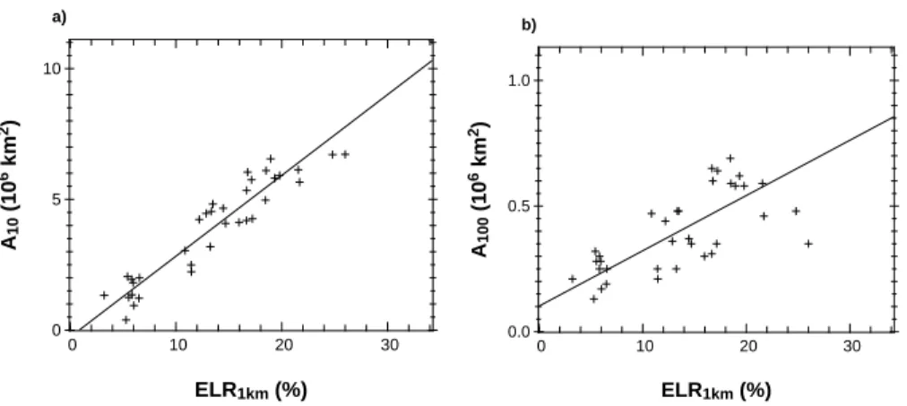
with ELR1km, versus how much remains near the source, quantified using A10 (or A1 orA100). Export of a significant fraction of the tracer mass to far away from the source will tend to dilute the tracer near the source, and result in smaller regions with elevated densities. Thus, one might at first expectA10 to be anti-correlated with ELR1km. Fig-ure7shows, however, that according to our calculations this is not the case. Instead, 25

for the τ=10 d tracers, A10 and even A100 are relatively well-correlated with ELR1km (the plots show the relationships between the values of each metric, with correlation coefficients of r2=0.91 and r2=0.60, respectively; for the ranks, the correlations are similar, withr2=0.87 and r2=0.56, respectively).

(25)

ACPD

Full Screen / Esc

The cause of this correlation betweenA10 and ELR1km is vertical transport. Tracer dispersion occurs in both the horizontal and the vertical. The importance of the verti-cal component was noted earlier. The results in this section show that for most of the MPCs, the transport into the free and upper troposphere, rather than long-range hor-izontal transport, which is primarily responsible for diluting the surface-layer pollutant 5

levels near their source locations. This is particularly the case for theτ=10 d tracers, for which the correlations with ELR1kmare mostly better than those for the τ=1 d and τ=100 d tracers. Since convective mixing time-scales in the atmosphere are of the or-der of 10 days (WMO,2002), it can be expected that regional variations in convection will have the largest effect on tracers with lifetimes in this range (e.g., O3 and sev-10

eral types of aerosols). For very short lifetimes, only a relatively small amount can be mixed out of the BL, while for much longer lifetimes, the tracers become close to being well-mixed, and thus again convection will play less of a role in either of these cases. Indeed, for the_{τ=1 d tracers, A}₁₀₀is only weakly correlated with ELR_1km(r2=0.1), and for theτ=100 d tracers, the only case is found for which the anticipated anti-correlation 15

does hold, namely between A1 and ELR1km (with r=−0.78). However, for the other combinations of threshold and lifetime, a significant positive correlation is computed, indicating the importance of vertical mixing in determining both pollution buildup and long-range low-level export for a wide range of tracer lifetimes.

4 Conclusions

20

This study has taken steps towards developing an overall understanding of the charac-teristics of pollutant outflow, long-range pollutant export and regional pollution buildup for emissions from major population centers (MPCs) distributed around the world. Un-like several previous studies with global models (e.g.,Stohl et al.,2002;Lawrence et al., 2003a;Pfister et al.,2004), which have focused on emissions from various continental-25

scale regions (e.g., Europe), the MPCs here have been represented as large point sources of artificial tracers with different lifetimes. The focus here has been on regional

(26)

ACPD

Full Screen / Esc

EGU scales (∼100–1000 km) to continental scales (>1000 km), which are appropriate for a

global model; it would also be interesting to have the insights from a similar compara-tive study of local pollution buildup on the scales of 100 km or less around MPCs, but this would require a multitude of simulations with a mesoscale model, or a global model using meteorological analysis data at a resolution that would be very computationally 5

intensive with this large number of tracers.

For this study, we have developed a new approach to looking at the comparative characteristics of pollutant dispersion from MPCs, by defining a set of various metrics targeting examination of different outflow and regional buildup characteristics. In princi-ple, the same approach could be applied to future model studies of other source types, 10

such as forest fires (e.g., Heald et al., 2003) and power plants (e.g., Marufu et al., 2004). Using these metrics, we arrived at the following key conclusions:

1. Long-range near-surface pollutant export is generally strongest in the middle and high latitudes, especially for Moscow and other source locations in Eurasia; 2. On the other hand, pollutant export to the upper troposphere is greatest in the 15

tropics, especially from Jakarta and other southeast Asian MPCs, due to transport by deep convection;

3. A large fraction of the chosen MPC source locations reflect the tendency for major cities to develop near coasts, which is in turn reflected in the results; for instance, the mean amount of long-range low-level pollutant export over land is only half as 20

large as the total export over land and sea;

4. Not only are there order of magnitude interregional differences, such as between low and high latitudes, but also often substantial intraregional differences, for in-stance between the sources in western India and Pakistan versus eastern India and Bangladesh;

25

5. While most source locations only show a moderate seasonal variability in the out-flow intensity and geographical distribution, particularly large seasonal differences

(27)

ACPD

Full Screen / Esc

are calculated especially for Asian cities like Delhi which are affected by the wind reversals and changes in convective activity accompanying the monsoons; 6. Pollutant buildup to high surface layer densities in the region surrounding the

source point is more strongly influenced by vertical than horizontal transport: in particular, contrary to what one might initially expect, we find that efficient long-5

range low-level horizontal export (e.g., to beyond 1000 km) is not generally as-sociated with significantly depleted pollution levels immediately surrounding the source, rather the amount of long-range, low-level export is well-correlated with regional scale (<1000 km) exceedences of surface density thresholds; this im-plies in particular that more work is needed in parameterizing deep convection 10

well, along with other processes that vent air pollution from the BL, including diur-nal BL height changes and land-sea breeze effects;

7. Despite the large differences in the MPC outflow characteristics, no MPC can be considered to be free of the potential for either a local, regional, or continental polluting influence; instead this study brings out the tradeoffs between local and 15

regional near-surface pollutant buildup, low-level long-range export to neighboring states, and export to the UT and potentially the lower stratosphere, as a function of the source location, which may be of use in future policy development.

The key caveat to these results is of course that they are model-based. Since this study examines carefully-chosen artificial tracers with representative characteristics, 20

a direct comparison with observations is not possible. Nevertheless, as mentioned above, we have evidence through previous studies with MATCH-MPIC in comparison to field observations that the model is able to represent pollutant outflow well at these scales in many different geographical regions, including outflow from North America, Europe, and southern Asia.

25

As an outlook, there are several questions which could be addressed in future stud-ies, either with comparable models to MATCH, or after further model developments (e.g., substantial improvements in resolution or transport parameterizations), which

(28)

ACPD

Full Screen / Esc

EGU would add to the initial overview of MPC regional pollution potentials developed in this

study, for instance:

– What additional information could be gained if the tracer results were convolved

with maps of population or agricultural distributions?

– How do physical deposition processes (surface uptake and precipitation

scaveng-5

ing) affect the pollution potentials, and what additional metrics might be sensible for examining the variability in regional deposition intensities?

– How do the long-range export potentials differ, especially for shorter-lived gases,

when they are released above the surface layer (e.g., at a few hundred meters altitude from tall smoke stacks)?

10

– What is the effect of the tendency of many real trace gases and aerosols to have

increasing lifetimes at greater altitudes?

– How great is the interannual variability in the pollution potential metrics?

– How do the regional pollution potentials change with future changes in climate

and meteorology? 15

– How do the results depend on the model resolution, and eventually on the ability

to better resolve orographic features and small-scale circulation effects such as the land-sea breeze (particularly relevant for the many coastal MPCs) and the urban heat island (which will particularly enhance local vertical mixing)?

Finally, since similar future studies would still often be necessarily model-based, 20

it would be worthwhile to consider a model intercomparison exercise to help make the results more robust, and to elucidate where the largest uncertainties in the model results are. A particularly enlightening step would be to involve regional models in such an intercomparison, in which the regional models would simulate MPC tracers which exactly replicate those used in the global models, i.e., emitted uniformly over a 25

(29)

ACPD

Full Screen / Esc

region representing the global model grid cell for each MPC, and with the same decay constants. This would especially help to document how future improvements in the parameterizations of vertical mixing by boundary layer diffusion and deep convection influence the computed characteristics of MPC pollutant dispersion.

Acknowledgements. We enjoyed early discussions on this and our related megacities work

5

with P. Crutzen and J. van Aardenne, and we acknowledge P. Rasch for the long-term support of MATCH. This work was largely supported by funding from the German Ministry of Education and Research (BMBF), project 07-ATC-02.

References

Chameides, W. L., Kasibhatla, P. S., Yienger, J., and II, H. L.: Growth of continental-scale

10

metro-agro-plexes, regional ozone pollution, and world food production, Science, 264, 74– 77, 1994. 13325

Crutzen, P. J. and Lawrence, M. G.: The Impact of Precipitation Scavenging on the Transport of Trace Gases: A 3-dimensional Model Sensitivity Study, J. Atmos. Chem., 37, 81–112, 2000.

13339

15

de Foy, B., Varela, J. R., Molina, L. T., and Molina, M. J.: Rapid ventilation of the Mexico City basin and regional fate of the urban plume, Atmos. Chem. Phys., 6, 2321–2335, 2006,

http://www.atmos-chem-phys.net/6/2321/2006/. 13327

Emberson, L., Ashmore, M., Murray, F., Kuylenstierna, J., Percy, K., Izuta, T., Zheng, Y., Shimizu, H., Sheu, B., Liu, C., Agrawal, M., Wahid, A., Abdel-Latif, N., van Tienhoven, M.,

20

de Bauer, L., and Domingos, M.: Impacts of air pollutants on vegetation in developing coun-tries, Water, Air Soil Pollut., 130, 107–118, 2001. 13325

Ganguly, D., Jayaraman, A., Rajesh, T. A., and Gadhavi, H.: Wintertime aerosol properties during foggy and nonfoggy days over urban center Delhi and their implications for shortwave radiative forcing, J. Geophys. Res., 111, D15217, doi:10.1029/2005JD007029, 2006. 13341

25

Gros, V., Williams, J., van Aardenne, J. A., Salisbury, G., Hofmann, R., Lawrence, M. G., von Kuhlmann, R., Lelieveld, J., Krol, M., Berresheim, H., Lobert, J. M., and Atlas, E.: Origin of anthropogenic hydrocarbons and halocarbons measured in the summertime European