Distribution network optimization in the uniform rental industry

Distribution Network Optimization in the Uniform Rental Industry

by

Ann-Marie Chopyak

Bachelor of Science, Business Administration, Boston University, 2008 and

Haotian Lee

Bachelor in Business Administration, University of Texas, 2011

SUBMITTED TO THE ENGINEERING SYSTEMS DIVISION

IN PARTIAL FULFILLMENT OF THE REQUIREMENTS FOR THE DEGREE OF

MASTER OF ENGINEERING IN LOGISTICS

AT THE

MASSACHUSETTS INSTITUTE OF TECHNOLOGY JUNE 2015

ARCHIVES

MASSACH ISETT- rT!NSTIJTE

IUL

16

2015

LIBRARo IES

C 2015 Ann-Marie Chopyak and Haotian Lee. All rights reserved.

The authors hereby grant to MIT permission to reproduce and to distribute publicly paper and electronic copies of this thesis document in whole or in part in any medium now known or

hereafter created.

Signature of Author...Signature

Signature of Author...Signature

redacted

Master o9fngineenng in LAg2tics Program, Engineering Systems Division Certified by...Signature

redacted

... Ma 8, 201

Sigr

Dr. Bruce C. Arntzen Executive Director, Supply Chagin )ayagement Program

iatu re red acted

11

.... . . . .

(/ Dr. Yossi Sheffi Director, Center for Transportation and Logistics Elisha Gray II Professor of Engineering Systems Professor, Civil and Environmental Engineering

Distribution Network Optimization in the Uniform Rental Industry

by

Ann-Marie Chopyak and

Haotian Lee

Submitted to the Engineering Systems Division on May 8, 2015 in Partial Fulfillment of the Requirements for

the Degree of Master of Engineering in Logistics

Abstract

Optimization models are a commonly used tool to identify cost efficient network flows. Complexity increases when various products move across different paths and transportation modes within one network. To address the challenges posed by this complexity, this thesis develops a mixed integer linear programming model for a uniform rental company. The company's product families are routed through intermediary distribution centers, while others bypass these points and move directly to a regional distribution center. Various simulations were run with the objective of minimizing fixed costs, warehousing, inventory and transportation expenses. The function was constrained by flow balance, demand and capacity constraints. The optimal solution proposed a network that used less facilities than currently operated within the company, and some in new locations due to transportation cost savings. As volume increased, the network structure continued to shift further from the company's current structure. Demand increased the influence of variable rates, while transportation lane rates were a significant factor in every version of the model run.

Thesis Supervisor: Dr. Bruce Amtzen

Dedication

This paper is dedicated to my incredibly supportive friends and family, who encouraged me to chase my dreams in pursuing an advanced degree this year. To my husband, mother, brother, and Jen - thank you for all of your love and energy. To Brittany, Sam, and Brooke, thank you for all of the laughs and distractions amidst the endless hours of work.

-Anny

To my family, friends and SCM classmates, I could not have completed this journey without you. Thank you for all of your support along the way.

Acknowledgements

This project would not have been possible without the unwavering encouragement and guidance of so many.

We would like to thank the team at MIT for supporting and challenging us on a daily basis. Specifically, we would like to acknowledge our thesis advisor and program director, Dr. Bruce Arntzen, for his patience, wisdom and humor throughout the year.

We would also like to thank the incredible team at our sponsor company for providing

exceptional support and leadership. We are especially grateful to Kelly Blackburn, Dave Meyn, and Orlando McGee for outstanding management support and for pulling all of the internal resources necessary to develop the model.

Table of Contents

2.1. Supply Chain N etw ork D esign ... 11

2.2. M ethods for M odeling Supply Chains... 12

3. M ETHODOLOGY... 15

3.1. Sponsor Com pany Project D evelopm ent ... 16

3.1.1. Sponsor company Project Scope and Parameters ... 17

3.1.2. Cost Drivers ... 19

3.2. M odel D evelopm ent... 21

3.3. A pplication of the M odel... 22

4. R ESULTS ... 23

4.1. M odeling Fram ew ork... 24

4.2. The Company's Supply Chain Network Data ... 28

4.2.1. Product Fam ily D ata ... 28

4.2.2. Supplier D ata ... 29

4.2.3. D istribution Center D ata... 30

4.2.4. Rental Region D ata... 31

4.3. M odel Iterations ... 32

4.3.1. Current State M odel... 32

4.3.2. Finance optim ized m odel... 33 5

4.3.3. Five year costing optim ized m odel... 33

4.3.4. Increasing dem and m odels... 33

4.3.5. Only Variable Costs M odel ... 34

5. DISCUSSION... 36

5.1. Key Findings... 36

5.2. Recommendations for Model Structure and Analysis ... 37

5.2.1. Transportation Lim itations... 37

5.2.2. N etwork Lim itations ... 38

5.2.3. Dem and Considerations ... 38

6. CONCLUSION ... 39

6.1. Im plications for The Com pany ... 39

6.2. Takeaw ays and Future Developm ents ... 39

FIGURES

Figure 1 Multi-echelon distribution network model (Ding, Benyoucef, & Xie, 2009)... 12 Figure 2 Distribution maps for three of The Company's product families, from distribution center to ren tal facilities... 17

Figure 3 Mini Model (no IDC) layout ... 22 Figure 4 Product Family Flow Pattern... 28

TABLES

Table 1 Rental Region D em and Groupings ... 19

Table 2 D istribution Center Costs... 20

Table 3 M odel Param eters ... 24

Table 4 M odel Locations ... 25

Table 5 Capacity U nit Conversions ... 29

Table 6 Supplier Region Capacity ... 30

Table 7 Distribution Center Capacity and Costs ... 31

APPENDICES

1. INTRODUCTION

The importance of supply chain network analysis has grown significantly over the past decade as suppliers, plants, distributors, warehouses and customers have globalized. In 2012, spending in the US logistics and transportation industry totaled $1.33 trillion, or about 8.5% of the country's gross domestic product (Schulz, 2014). As the field gains importance, executives are modernizing their supply chains to optimize supply and demand.

A global uniform supply company, hereafter referred to as The Company, has partnered

with our team at MIT to examine its current supply chain operations and identify cost savings opportunities. The Company provided historical transportation data, distribution center infrastructure information, and sales figures. After examining the data, we suspected that the company could benefit from fully integrating disparate networks and streamlining operations. Therefore, the goal of our research was to develop a distribution network that optimizes the tradeoff between costs and customer service levels.

Our objective was to find the optimal distribution network layout for our sponsor company. The Company provided us with details surrounding supply and demand by product, capacity for their current DCs, and locations for expansion or new distribution centers. They also provided costs for the DCs and transportation lanes. Based on this information, we manipulated the products into groupings to simplify the complex network and built a model that would find the best way to minimize cost while still meeting demand.

1.2. Motivation

While this thesis specifically addresses The Company's distribution center network, the factors influencing the model's outcome are the same factors any company would require to optimize a similar network. The optimization model can balance distribution center fixed and variable costs with transportation costs to find the least expensive solution. The model can also tell a company how many distribution centers are needed to fulfill demand.

Section 1 provides an overview of our research question and thesis project. Section 2 provides a literature review and section 3 describes our methodology and approach. Section 4 explains the final model and its results, while section 5 discusses the outcome in further detail and provides further recommendations. Section 6 offers concluding thoughts.

2. LITERATURE REVIEW

We conducted a review of the literature related to optimization methods for supply chain networks in order to identify appropriate modeling techniques and identify constraints and parameters to include in the optimization model. After a brief overview of basic supply chain network structure in the following section, subsequent sections will review historical modeling methodologies, first observing model development (including setting objectives, variables and constraints) and then specific algorithms.

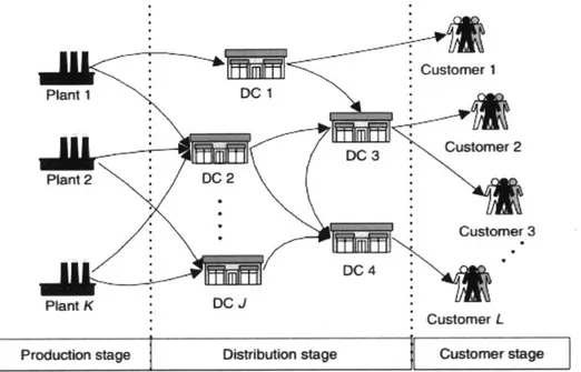
2.1.

Supply Chain Network Design

A common framework for illustrating a supply chain network design consists of three

Customer 1 Plant 1 DC I Customer 2 Plant 2 DC 2 Customer 3 Plant K DC J Customer L

Production stage Distribution stage Customer stage

Figure I Multi-echelon distribution network model (Ding, Benyoucef, & Xie, 2009)

Successful companies use their supply chain design as a strategic weapon by leveraging network modeling. The objective is to determine the best location and size for their facilities while seeking to minimize the total costs associated with the production, storage, and distribution activities, along with the total investment outlays to achieve the activity levels on the various links (Nagurney, 2010).

2.2.

Methods for Modeling Supply Chains

A recent technique used for analyzing supply chains is system-optimization models. Anna

Nagurney (2012) proposed this framework for network design to determine optimum capacity levels and product flows for manufacturing, storing and distributing at minimal total cost. This method is unique in that it considers capacity as design variables, allowing inputs to change during simulation. The need came about as mergers and acquisitions (M&A) activity trended upward after

the collapse of the economy in 2009. Therefore, this method is particularly useful for supply chain network integration in the case of M&A (Nagurney, 2010).

This method of modeling can be applied to various industries. For example, Jin, Yang, and He (2012) constructed a flow balance model while analyzing a Beijing agricultural product distribution center. The team began by building a deterministic demand model for the current system before factoring in demand variability. The goal was to minimize the sum of the fixed costs for each DC (referred to as a node), transportation costs for each lane, and penalty costs for not meeting demand. The model was constrained by flow balance restrictions and set supplier quantities. Ultimately, the researchers found that their model closely reflected the optimal scenario when applied to the Beijing agricultural business.

A different method for examining network design is the Petri net technique, which

emphasizes customer order fulfillment instead of more traditional financial metrics such as minimizing total system costs. System models are built upon colored Petri nets and used to incorporate product and process concerns into the supply chain configuration process (Zhang, You, Jiao, & Helo, 2009). These models are ideal for make to order (pull systems) supply chains where efficiently delivering custom products is a necessity.

Furthermore, just in time supply chains must also be modeled in their own unique way. In order to minimize costs in such networks, researchers have incorporated fuzzy logic into bi-objective mixed integer linear programming. This model integrates procurement, production and distribution plans under fuzzy supply, production and demand by considering cross-docking and direct shipments simultaneously (Ahmadizar & Zeynivand, 2014).

Considering many of the same variables and constraints as past researchers, Aikens' (1985) research diverges through creating a model to optimize a distribution network using defined flow balance. Although his method considers many of the same variables and constraints as the others, he also factors in side constraints, such as demand volatility, that could be included in a model. His research highlights the flexibility gained by incorporating or excluding many side constraints depending on the specific nature of the system being modeled. Ultimately, as the various different models work for various individual problems, Aikens indicates that the model and algorithm can vary widely within an optimization model. Aikens also explicitly assumes unlimited capacity for the distribution centers. In practical matters, it is unrealistic to consider unlimited capacity, as this would require tremendous physical space.

Owen and Daskin (1998) counter Aikens' unlimited capacity assumption and focus heavily on the strategic importance of facility locations and related costs. The authors suggest that not enough emphasis has been placed on the lasting costs and impacts of facility placement decisions. As there are sizeable expenses involved in opening, closing, or expanding a facility, these factors must be weighted heavily in any model.

The distribution network design problem can be solved in many ways. However, in-depth analysis suggests that researchers use a particular method on a far more consistent basis than the others: mixed integer programming. While this approach has been used for decades, in recent years there has been a growing awareness of the importance of incorporating reverse and closed-loop supply chain activities along with the traditional indicators (Ozceylan & Paksoy, 2012). The scope of our research precludes incorporating closed-loop activities. However, since our thesis partner

operates in the lease and rental services space, future projects analyzing detailed treatment of reverse logistics is recommended.

Although much research has already been completed on supply chain network design, there are two main gaps, which our thesis will address. Most work either optimizes cost and service levels on a strategic level, focusing on the physical structure of a network, or examines on an operational level emphasizing production planning and inventory management. Our model will reconcile the two approaches and optimize the intersection of costs and service levels. This combination of the two considerations is vital for successful implementation, as it will likely provide a more agreeable solution for different departments within the company. A decision that only benefits high level strategic planning without considering daily operational planning implications, or vice versa, is unlikely to receive full buy in from all internal parties, which is essential for success.

Lastly, restructuring a supply chain network requires making tough business decisions on opening and closing distribution centers. Department silos within organizations have led many researchers to omit working with the finance department to develop realistic costs associated with opening and closing these facilities. Our team will focus on establishing a mutual agreement between finance and operations when evaluating these financial metrics.

3. METHODOLOGY

An optimization model based on a linear program is a highly effective tool to find the optimal flow of goods through a network. (Shapiro, 2001.) Shapiro provides a detailed analysis of the spreadsheet options to optimize network flow problems using algorithms embedded in the

software. While the mathematical algorithms are highly complex, the objective function can nearly always be defined as the minimum or maximum feasible result for a company's primary goal. Such goals can include cost (minimization), revenue (maximization), or transit time

(minimization.) The objective function would be defined as the mathematical formula relating all the variables that contribute towards any one of these specific goals.

Microsoft Excel provides a foundation for a basic, high-level model and is often used to manage optimization models for academic and professional purposes. (Alfares, 2012; Barati, n.d.; Bjdrk & Mezei, 2014; Shaoyun & Honglin, 2011.) However, Excel does not have the capacity to handle over 200 decision variables (Standard Excel Solver, n.d.), so the program cannot optimize large distribution networks that contain many transportation lanes. Excel offers premium purchasable add-ons for model expansion; one add-on, WhatsBest!, is an effective optimization tool with more capacity. (Shapiro, 2001.) For this reason, we used WhatsBest! to optimize The Company's sizeable distribution network.

3.1.

Sponsor Company Project Development

The Company's primary goal is to analyze the cost of its current network and see whether relocating, expanding, and/or closing distribution centers would allow them to maintain the same

capacity for less cost. The Company and the thesis team worked collectively to develop a simplified representation of the distribution flow to gain an understanding of how the network could be feasibly optimized. Cost drivers, including the transportation rates, distribution center fixed costs, and distribution center holding costs, were then obtained and entered into the model for optimization.

3.1.1. SPONSOR COMPANY PROJECT SCOPE AND PARAMETERS

Data was primarily collected from The Company's historical accounting and

transportation financial records. Initial conversations to learn more about the company's network design, potential distribution center locations, and feasible shipping alternatives were held with the logistics, finance, and supply chain teams. Weekly calls supplemented these discussions to thoroughly define scope and potential restructuring of the supply chain network.

From these conversations, three divisions were determined "in-scope" for the project: First Aid & Safety, Facility Services, and Rental Garments. Though each division can ship to both the rental facilities and direct to customer, each has its own unique network. First Aid & Safety is distributed out of only one location, while Facility Services ships from two, and Rental Garments ships from eight separate distribution centers. Rental Garments also can ship through an intermediary distribution center before being shipped to its final distribution center for release to the rental facility. The Company's current distribution network is shown in Figure 2.

First Aid & Safety Distribution Ntok 1, ySrie Dsrt ewr

Rental Garrmont Disiribution Netwo

Having different network arrangements introduces system complexity, making

optimization of the network difficult for each product family. However, establishing multiple supply chains provides significant opportunity to enhance the network structure. For example, there is no secondary shipment location for First Aid & Safety, meaning if there were a natural disaster in Ohio, no First Aid & Safety products could be shipped. While splitting the inventory would avoid the risk associated with locating all products in one location, it would likely force the model to find a higher cost solution. Optimizing certain Rental Garments adds further complexity to the model by forcing some products through an intermediary distribution center

(IDC) due to safety stock needs or supplier shipping agreements. There is no flexibility to

eliminate these intermediary points, which increases system costs because additional transportation lanes are required.

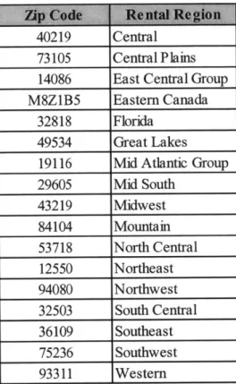
To mitigate some of this complexity, we worked with The Company to group similar product types, supplier regions, and rental facility regions together. Grouping together similar nodes and variables reduced the number of transportation lanes and product families in the model. The suppliers were simply grouped into The Company's three US three ports: Miami, Seattle, and Newark. The rental region categories can be seen in Table 1.

Table I Rental Region Demand Groupings

40219 Central

73105 Central Plains

14086 East Central Group

M8ZlB5 Eastern Canada

32818 Florida

49534 Great Lakes

19116 Mid Atlantic Group

29605 Mid South 43219 Midwest 84104 Mountain 53718 North Central 12550 Northeast 94080 Northwest 32503 South Central 36109 Southeast 75236 Southwest 93311 Western

Finally, The Company decided to assume flat supply and demand from its historical data and to utilize historical shipment flow for the network optimization. This decision simplifies the model as it does not introduce the risk associated with forecasted regional growth but may force The Company to run a similar model in the future if there are projected shifts in regional

demand.

3.1.2. COST DRIVERS

Data for the costs were primarily collected from The Company's historical accounting and transportation financial records. Rates for existing lanes were pulled from The Company's freight payment system, and rates for new lanes were obtained through quotes from the current carrier base. The model did not consider mode switching, which simplified the lane rate

procurement for new lanes. However, this also limited the optimization as no aggregation and consolidation cost savings opportunities could be created.

For the distribution center costs, The Company selected new potential distribution center locations to add to their current network based on internal assumptions and preferences. The

Company's finance team calculated detailed costs for distribution center operations, and for opening new distribution centers and closing and expanding current distribution centers in table 2. Costs for relocating products were ignored, as The Company assumed it would burn off all inventory rather than move finished goods from one facility to another.

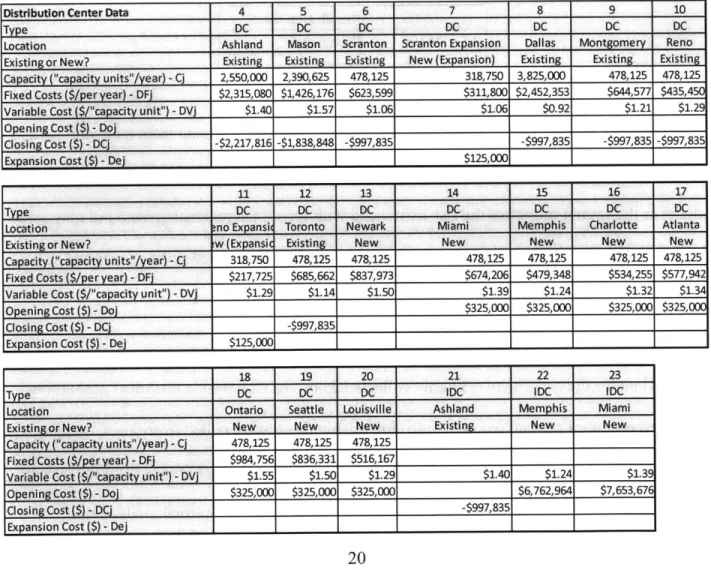
Table 2 Distribution Center Costs

Distribution Center Data 4 5 6 7 8 9 10

Type DC DC DC DC DC DC DC

Location Ashland Mason Scranton Scranton Expansion Dallas Montgomery Reno Existing or New? Existing Existing Existing New (Expansion) Existing Existing Existing Capacity ("capacity units"/year) - Cj 2,550,000 2,390,625 478,125 318,750 3,825,000 478,125 478,125 Fixed Costs ($/per year) - DFj $2,315,080 $1,426,176 $623,599 $311,800 $2,452,353 $644,577 $435,4 Variable Cost ($/"capacity unit") - DVj $1.40 $1.57 $1.06 $1.06 $0.92 $1.21 $1.29

Opening Cost ($) -Doj I

_ I I I_ I

Closing Cost ($) - DCI -$2,217,816 -$1,838,848 -$997,835 -$997,835 -$997,835 -$997,835

Expansion Cost ($) -Dej ... a- 1 $125,000 En

11 12 13 14 15 16 17

Type DC DC DC DC DC DC DC

Location no Expansi. Toronto Newark Miami Memphis Charlotte Atlanta

Existing or New? w (Expansic Existing New New New New New

Capacity ("capacity units"/year) - C 318,750 478,125 478,125 478,125 478,125 478,125 478,125

Fixed Costs ($/per year) - DFj $217,725 $685,662 $837,973 $674,206 $479,348 $534,255 $577,942

Variable Cost ($/"capacity unit") - DVj $1.29 $1.14 $1.50 $1.39 $1.24 $1.32 $1.34

Opening Cost ($) -Doj 1 _ $325,000 $325,000 $325,000 $325,00C

Closing Cost ($) -DCj 1 -$997,835 1 1

Expansion Cost ($) -Dej $125,000 1 1 1

18 19 20 21 22 23

Type DC DC DC IDC IDC IDC

Location Ontario Seattle Louisville Ashland Memphis Miami

Existing or New? New New New Existing New New

Capacity ("capacity units"/year) - Cj 478,125 478,125 478,125 Fixed Costs ($/per year) - DFj $984,756 $836,331 $516,167

Variable Cost ($/"capacity unit") -DVI $1.55 $1.50 $1.29 $1.40 $1.24 $1.39

Opening Cost ($) -Doj $325,000 $325,000 $325,000 $6,762,964 $7,653,676

Closing Cost ($) -DCj -$997,8351

3.2.

Model Development

In the network development, specific notation was used to define each node (a stock point, such as a supplier, distribution center, or rental facility) and leg (a flow, such as a Less Than Truckload or Truckload lane rate, as well as the units moving along that lane.) I represents an origin node, meaning a point from which any shipment could depart. For this reason, either the supplier or distribution center could be treated as an origin node. J, similarly, is a destination node and could be a distribution center or rental facility. K is a product family, as defined by the team in regard to unit capacity. The list of notations used for The Company's model can be found in the following Results section in Table 3 - Model Parameters.

The optimization contained formulas to force flow balance along the arcs (what goes in must come out), demand fulfillment, non-negativity, and supplier capacity limitations. A big M variable was also used to link the binary variable representing whether or not a distribution center was opening, closing, or expanding to the associated costs. Finally, the model was set to minimize the sum of the total transportation costs, distribution center costs, and handling costs. To test our calculations before inputting The Company's data, we ran some smaller scale models. We first developed a mini model, which will be reviewed in detail in the next

subsection, to reflect the supplier to distribution center to rental flow that First Aid & Safety and Facility Services utilize, as they bypass the intermediary distribution center. We created a second mini model to capture the Rental Garment flow through the intermediary distribution center. With both of these models successfully yielding optimal results, we combined them into one model that directed the Rental Garments to the intermediary distribution center and forced the First Aid & Safety and Facility Services products to bypass the intermediary distribution point.

3.3.

Application of the Model

To illustrate the application of the model, the following section provides an example using simplified parameters to test the flow balance and model optimization.

Prior to inputting the specific transportation rates, costs and constraints, a mini model was run to test the network flow balance and parameters. The model contained theoretical numbers to represent demand, capacity, lane rates, and distribution center opening, closing, and expansion costs with fewer product families and excluding the intermediary distribution center.

Figure3 MiniModeD4no layou *DC 404 DC5-EpmmPV,C

DC6 E=WS

DC,~wwDV L i , 4 ka

k~~praihi~~tfamiy DCS D.'DF

Figure 3 Mini Model (no JDC) layout

After conceptualizing the mini model, simple units were arbitrarily defined to easily comprehend the model and its results. To accurately account for handling costs across various product

families, a unit of product (e.g. pair of shoes, one shirt) was standardized into a "capacity unit." From the given data, constraints were defined. By placing a parameter that forced the number of capacity units going into each node to be the same as the number coming from each

forced to be greater than or equal to the rental demand to ensure that demand was completely fulfilled for each product family. Non-negativity constraints were set on the distribution center and origin shipment points. Finally, the big M constraint linked the DC operation (including opening, closing, or expanding) to its relevant costs. Big M was set at $1,000,000 for this model.

Based on the constraining formulas, the mini model yielded a simple solution that recommended maintaining the two open facilities and not making any other changes. This result was expected, given the high costs of changing DC locations and the random selection of freight rates. From this mini model, a larger model can be extrapolated to include more product families, regions, intermediary DCs, and additional lane rates while still holding the same constraints.

Section 3 summarized the model development process used to answer the thesis objective of identifying a lower cost distribution network. Section 4 will address the larger model and its results. By running various models testing the effects of certain constraints, The Company can analyze aspects of its business to find ways to relax constraints and improve its optimal solution.

4. RESULTS

The mini model described in the Methodology section was built to gain understanding of how to represent and analyze The Company's supply chain network. A comprehensive binary mixed integer linear programming model, built based on the mini model, accurately represented The Company's end-to-end network design by using historical data and current network

infrastructure specifications. It integrates location and capacity options for distribution centers, product family assignment and product flow. This model was used to run the simulations described in this section and to develop our recommendation. Each iteration relaxes different constraints, resulting in the three different variations for solving the problem.

4.1.

Modeling Framework

All of our simulation runs solve for the same objective function with similar constraints.

The simulation consisted of parameters, locations, an objective function, and constraints.

Table 3 Model Parameters

i Supplier Node

-IDC Node

-I DC Node

m Rental Region Node

-k Product Family

X1k, XkI, Xjk], XkIm Product Flow Units

Sik Supplier Capacity Units/Year/Family

Ak Product Family Units per Units/Capacity Unit Capaci Unit

Bk Pounds per Product Pounds Family Unit

Ci, CI IDC, DC Capacity Units/ear DFi, DFI IDC, DC Fixed Costs $/Year DVi, DV IDC, DC Handling Cost $/"Capacity Unit"

DO, DOI IDC, DC Opening Cost $

DCi, DC1 ID, DC Closing Cost $ DE,, DE IDC, DC Expansion $

Cost

RDmk Rental Region Demand Units/Year/Family

RT,,, R'Iim TL Freight Rate $/Pound RLL, RL0 LTL Freight Rate $/Pound

RLim

Fi / F1 Binary Decision Variable for IDC,DC

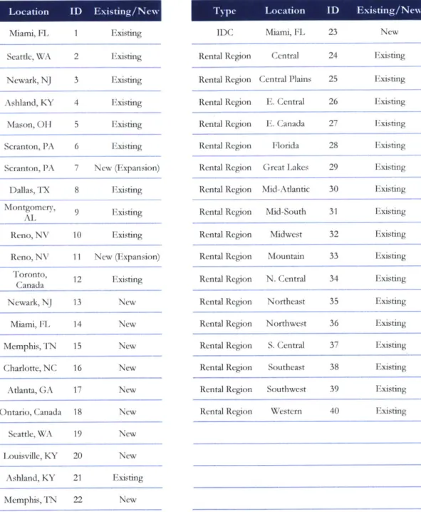
Table 4 Model Locaiions

Suppher _{Miami, FL 1 Existing} Region

Supplier Seattle, WA 2 Existing

R.gI Aon

Supplier Newark, NJ 3 Existing

DC Ashland, KY 4 Existing

DC Mason, OH 5 Existing

DC Scranton, PA 6 Existing

DC Scranton, PA 7 New (Expansion)

DC Dallas, TX 8 Existing

DC Montgomery, 9 Existing

AL __

DC Reno, NV 10 Existing

DC Reno, NV 11 New (Expansion)

DC Toronto, _Canada 12 Existing

DC Newark, NJ 13 DC Miami, Fl. 14 New New DC Memphis, TN 15 New DC Charlotte, NC 16 New DC Atlanta, GA 17 New

DC Ontario, Canada 18 New

DC Seattle, WA 19 New

DC Louisville, KY 20 New

IDC Ashland, KY 21 Existing

IDC Miami, FL 23 New

Rental Region Central 24 Existing

Rental Region Central Plains

Rental Region E. Central

Rental Region E. Canada

Rental Region Florida

Rental Region Great Lakes

25 Existing

26 Existing

27 Existing

28 Existing

29 Existing Rental Region Mid-Atlantic 30 Existing Rental Region Mid-South 31 Existing Rental Region Midwest 32 Existing Rental Region Mountain 33 Existing Rental Region N. Central 34 Existing Rental Region Northeast 35 Existing Rental Region Northwest 36 Existing Rental Region S. Central 37 Existing Rental Region Southeast 38 Existing Rental Region Southwest 39 Existing Rental Region Western 40 Existing

IDC Memphis, TN 22 New

" Objective Function: Minimize costs while satisfying demand from each customer region

" Constraints:

" Must maintain flow balance for intermediate nodes

* Demand must be met for each customer region * Flow along each arc cannot be negative

* Product families must flow through designated network path (e.g. utilization of

IDC or direct shipments to regional DC)

* Product families must use designated transportation mode (e.g. LTL or TL) * Capacity at each IDC and DC cannot be exceeded

* Linking constraints are needed for all IDC and DCs

o Binary variables for each DC will be used to determine whether or not to use it. 1 represents yes, 0 for no.

o Incorporate big M * Non-Negativity

Thus, the model can be stated as follows:

Objective Function:

Min:

Z

4 8 44 + + X(DVj) (DV ) + (DV) + RLiXijk Bk Ak 1 k& ___ k=1 ijk=5 0, k=1 j' k=1 i~j 8 4 + RLilXl kBk + RLjiXj1kBk + RLlmXlmkBk k=7 il k=1 j,1 k=1-4,7,8 1,m 6 6 + RTiiXi₁,Bk + RTlmXlmkBk k=5 iji k=5 1,m Subject To: , Xp --

Y

Y

m MBalance

Xk = YXm fork = 5 - 8andVI

Xlmk RDmk V m, k

}

]

r22

I2k=5,k

Y2

r

}

}

}

for all ilk for all lmk

4.2.

The Company's Supply Chain Network Data

Historical data received from The Company's supply chain team provided the input and constraints for the model.

4.2.1. PRODUCT FAMILY DATA

The Company's product line was allocated into three product families representing eight basic item types. Each product family was assigned a network path and transportation mode within the company's supply chain network. These designated paths are shown in Figure 4.

Rental

Supplier Region (I IDC (j DC (1) Rental Region (nv Rental Product Flow Conditions

1-4 yes LTL

Facility Services (FS)

Supplier Region (i DC 1) Rental Region (m FS Product Flow Conditions

5-6 No Truckload First Aid & Safety (FAS)

Supplier Region (i) DC 0) Rental Region (m;

FAS Product Flow Conditions - No LTL

Rental product family items must flow through an IDC and use LTL freight. Facility services product family items (restroom cleaning supplies, mat service, mops, towels) bypass the

IDC and ship directly to regional DCs using TL freight. The FAS (First Aid & Safety) product

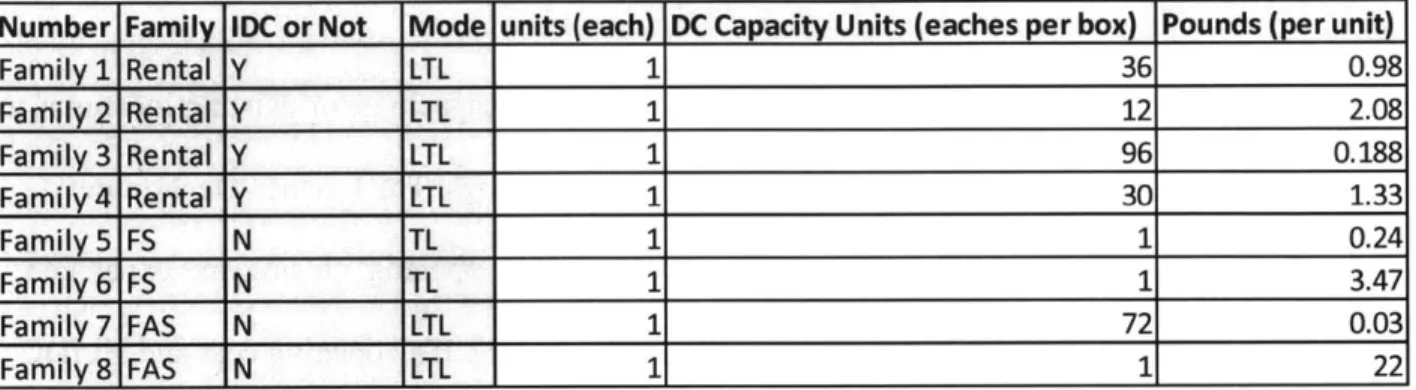
family items also bypass the IDC but ship directly to regional DCs using LTL freight. Table 5 provides capacity unit translations for each product family item.

Table 5 Capacity Unit Conversions

Number Family IDC or Not Mode units (each) DC Capacity Units (eaches per box) Pounds (per unit)

Family 1 Rental Y LTL 1 36 0.98 Family 2 Rental Y LTL 1 12 2.08 Family 3 Rental Y LTL 1 96 0.188 Family4 Rental Y LTL 1 30 1.33 Family 5 FS N TL 1 1 0.24 Family 6 FS N TL 1 1 3.47 Family 7 FAS N LTL 1 72 0.03 Family 8 FAS N LTL 1 1 22 4.2.2. SUPPLIER DATA

Product flowing into The Company's supply chain network was modeled to arrive from three supplier regions. For modeling purposes, supplier regions are synonymous with ports. The ports of Miami, Seattle and Newark are the three most heavily utilized import locations for the company's distribution of goods.

Table 6 shows the number of units flowing into the system by supplier region and product family. Again, units are converted into standard capacity units to standardize accounting for DC handling costs.

Table 6 Supplier Region Capacity

"capacity units" Supplier Data Supplier Region 1 Supplier Region 2 Supplier Region 3 Sum of units (standard boxes)

Port Miami Seattle Newark

Capacity (units/year/family) - Sik Family 1 11,843,760 1,863,498 99,825 13,807,083 383,530

Capacity (units/year/family) - Sik Family 2 419,658 86,378 803,345 1,309,381 109,115

Capacity (units/year/family) -Sik Family 3 12,179 67,980 - 80,159 835

Capacity (units/year/family) - Sik Family 4 11,099,118 10,772 1,136,707 12,246,597 408,220 Capacity (units/year/family) - Sik Family 5 242,915 226,017 93,383 562,315 562,315

Capacity (units/year/family) - Sik Family 6 2,025,967 353,058 929,406 3,308,431 3,308,431

Capacity (units/year/family) - Sik Family 7 21,461,665 3,958,429 322,057,816 347,477,910 4,826,082 Capacity (units/year/family) - Sik Family 8 331,268 53,518 2,749,465 3,134,251 3,134,251

4.2.3. DISTRIBUTION CENTER DATA

The Company provided distribution center throughput capacities for existing locations, as well as estimated expansion capacities for potential new buildings. The Finance Department assisted in generating realistic DC expenses for fixed, variable, opening, closing and expansion costs for each existing and expansion warehouse location. As the IDC opening cost and all IDC and DC closing costs were quite high, we allocated them over a five year period. These figures can be found in Table 7.

Table 7 Distribution Center Capacity and Costs

Distribution Center Data 4 5 6 7 8 9 10

Type DC DC DC DC DC DC DC

Location Ashland Mason Scranton Scranton Expansion Dallas Montgomery Reno

Existing or New? Existing Existing Existing New (Expansion) Existing Existing Existing

Capacity ("capacity units"/year) -C 2,550,000 2,390,625 478,125 318,750 3,825,000 478,125 478,125 Fixed Costs ($/per year) - DFj $2,315,080 $1,426,176 $623,599 $311,800 $2,452,353 $644,577 $435,4 Variable Cost ($/"capacity unit") - DVj $1.40 $1.57 $1.06 $1.06 $0.92 $1.21 $1.2

Opening Cost ($ - Doi I

Closing Cost ($) -DCj -$443,563 -$367,770 -$199,567 1 -$199,567 -$199,567 -$199,567

Expansion Cost ($) -Dej $125,000 1 1

11 12 13 14 15 16 17

Type DC DC DC DC DC DC DC

Location no Expansi Toronto Newark Miami Memphis Charlotte Atlanta

Existing or New? w (Expansic Existing New New New New New

Capacity ("capacity units"/year) - Cj 318,750 478,125 478,125 478,125 478,125 478,125 478,125

Fixed Costs ($/per year) - DFj $217,725 $685,662 $837,973 $674,206 $479,348 $534,255 $577,942

Variable Cost ($/"capacity unit") - DVj $1.29 $1.14 $1.50 $1.39 $1.24 $1.32 $1.34

Opening Cost ($) -Doj $325,000 $325,000 $325,000 $325,0C

Closing Cost ($) - DCj -$199,567

Expansion Cost ($) -Dej $125,0001

18 19 20 21 22 23

Type DC DC DC IDC IDC IDC

Location Ontario Seattle Louisville Ashland Memphis Miami

Existing or New? New New New Existing New New

Capacity ("capacity units"/year) - Cj 478,125 478,125 478,125

Fixed Costs ($/per year) - DFj $984,756 $836,331 $516,167

Variable Cost ($/"capacity unit") - DVj $1.55 $1.50 $1.29 $1.40 $1.24 $1.39

Opening Cost ($) -Doj $325,000 $325,000 $325,000 $1,352,593 $1,530,735

Closing Cost ($) - DCj 1 -$199,567 1

Expansion Cost ($) -Dej I I I

Additionally, we had to consider the flow through the distribution center. The Capacity figures in Table 8 represent each facility's flow. To calculate this figure, we identified the number of trucks and less than truckload that each dock could handle per day and multiplied by the number of days worked each year and the number of capacity units that can fit on a truck.

4.2.4. RENTAL REGION DATA

Customer locations, known as rental regions in the model, were assigned to 17 geographic areas in the country. Customer demand for each rental region is shown for the 17 product families in Table 8.

Table 8 Rental Region Demand

Rental Location Data Rental Region 24 Rental Region 25 Rental Region 26 Rental Region 27 Rental Region 28 Rental Region 29 Region Central Central Plains East Central Group Eastern Canada Florida Great Lakes Rental Demand (units/year/family) -RDjk k=1 1,410,422 1,379,311 1,258,819 812,976 1,272,931 2,255,883

Rental Demand (units/year/family) -RDjk k=2 151,168 129,250 152,922 191,257 29,902 176,266

Rental Demand (units/year/family) -RDjk k=3 5,537 3,954 5,284 54,877 3,107 12,910

Rental Demand (units/year/family) -RD~k k=4 1,218,750 1,039,790 1,208,835 636,133 1,120,501 2,118,144

FS Demand (units/year/family) -RDjk k=5 43,715 40,938 29,448 29,953 34,276 52,491

FS Demand (units/year/family) -RDjk k=6 350,178 317,883 302,247 90,565 193,213 625,704 FAS Demand (units/year/family) -RDjk k=7 420,010 - - - -

-FAS Demand (units/year/family) -RDjk k=8 34,505 - - - -

-Rental LocatIon Data Rental Region 30 Rental Region 31 Rental Region 32 Rental Region 33 Rental Region 34 Rental Region 34 Rental Region 35 Region Mid Atlantic Group Mid South Midwest Mountain North Central North Central Northeast Rental Demand (units/year/family) -RDjk k=1 2,827,623 1,409,233 1,477,271 1,133,063 1,771,793 1,771,793 1,209,953

Rental Demand (units/year/family) -RDik k=2 266,320 139,513 106,638 220,583 190,679 190,679 122,656

Rental Demand (units/year/family) -RDjk k=3 22,053 4,342 16,171 6,064 11,679 11,679 12,288

Rental Demand (units/year/family) -RDjk k=4 2,596,238 1,384,384 1,364,005 863,107 1,471,072 1,471,072 1,034,791 FS Demand (units/year/family) -RDjk k=5 77,625 38,603 30,864 55,449 56,902 56,902 35,792

FS Demand (units/year/family) -RDjk k=6 660,711 158,797 345,476 253,796 587,424 587,424 354,604

FAS Demand (units/year/family) -RDjk k=7 - - - - 552,229 552,229 903,448

FAS Demand (units/year/family) -RDjk k=8 - - - - 21,952 21,952 47,187

Rental Location Data Rental Region 36 Rental Region 37 Rental Region 38 Rental Region 39 Rental Region 40 Rental Region 39 Rental Region 40 Region Northwest South Central Southeast Southwest Western Southwest Western Rental Demand (units/year/family) -RDjk k=1 842,142 1,123,571 1,547,134 1,863,436 1,272,499 1,863,436 1,272,499

Rental Demand (units/year/family) -RDjk k=2 146,377 116,541 125,453 182,686 121,132 182,686 121,132

Rental Demand (units/year/family) -RDjk k=3 3,035 3,837 10,178 4,044 3,289 4,044 3,289

Rental Demand (units/year/family) -RD~k k=4 578,749 1,032,158 1,476,264 1,342,574 1,026,717 1,342,574 1,026,717

FS Demand (units/year/family) -RDjk k=5 45,184 35,975 41,689 59,525 46,392 59,525 46,392

FS Demand (units/year/family) -RDIk k=6 286,937 276,534 286,470 458,946 188,396 458,946 188,396

FAS Demand (units/year/family) -RDjk k=7 - - 667,946 - 799,759 - 799,759 FAS Demand (units/year/family) -RDjk k=8 - - 44,870 - 29,837 - 29,837

4.3.

Model Iterations

Once the model was built, with the mini model constraints and the data provided by The Company, we ran iterations to analyze the model's behavior and key variables and constraints.

4.3.1. CURRENT STATE MODEL

To ensure that the model reflected The Company's business and constraints, we first had to train the model. This involved forcing all of the new distribution center locations closed, to see if the volume would flow through the model network in a way that approximately matched The Company's current product flow. The Company acknowledged that minimal mathematical and financial studies had been done when opening new locations or shifting volume, so that the model would likely run a more cost efficient operation than the company currently does.

The model successfully allocated products throughout the current DCs, with the most volume running through Ashland, as it also serves as the only IDC for The Company. This is consistent with current operations, but proved to not be the optimal solution

4.3.2. FINANCE OPTIMIZED MODEL

Two versions of the initial optimization model were run to account for finance's preference to recognize all opening, closing, and expansion costs in the first year. The model is a single-period model, which means it cannot distinguish one-time costs from annual costs. With opening costs as high as $7 million, this means the model would have to find savings exceeding this amount to validate opening a new IDC. As expected, when we ran this iteration, the model did not open any new locations. The optimized solution filled every DC to maximum flow capacity with the exception of Mason, which has a capacity similar to Ashland's but higher variable costs and cannot also operate as an IDC.

4.3.3. FIVE YEAR COSTING OPTIMIZED MODEL

To truly see the impact of the optimization tool, we spread the IDC opening and all of the

IDC and DC closing costs over five years. This provides the model more decision making

flexibility, as it only needs to find savings of a fifth of an opening or closing cost in order to validate changes to the network. This model opened Miami as a new DC and IDC, and closed Mason and Toronto. The reason for the shift was the transportation savings, as more supplier volume comes through Miami than either of the other ports.

4.3.4. INCREASING DEMAND MODELS

Continuing with the IDC opening cost and the IDC and DC closing cost five year allocation, we ran iterations for a 10% and a 20% increase in demand. The difference between the

two scenarios was unexpected, but illuminated some crucial points for The Company to consider in mapping its future.

With 10% demand growth across all product families and regions, the model found a similar solution to the Five Year Costing Optimized Model. Additional demand was placed into the Ashland IDC and into Atlanta. The model also kept Toronto open, which it had not done in the model based on historical demand.

When we increased demand an additional 10% across the board, there was a sizeable shift toward consolidation in larger facilities. Ashland, Scranton, Reno, and Dallas were filled to capacity, while Miami was opened as an IDC and also completely filled. Mason, for the first time, was also nearly filled to capacity. Toronto, though kept open at the 10% demand increase, was closed at the 20% increase, as paying the additional fixed costs for its smaller size did not compensate for the increased variable costs to put all of the additional volume in Mason.

4.3.5. ONLY VARIABLE COSTS MODEL

To continue analyzing the impact of variable costs on the model, we ran a simulation excluding all fixed, opening, closing, and expansion costs. Again, the IDC opening costs and the

IDC and DC closing costs were spread over a five year time period, and demand was reset to its

historical levels. The solution spread the products widely across a mix of new and existing DCs and IDCs. Ashland was used minimally, and Mason not at all. Scranton and Reno were expanded, and many of the smaller DCs were filled to capacity. Dallas, the largest DC, was still also filled in entirety due to its extremely low variable costs. Newark, Miami, Seattle, Charlotte, and Louisville were also opened due to their lower variable costs, and in the case of Seattle and Miami, due to their close proximity to the supplier ports.

4.4. Recommendation

The Company's current network is sufficient for its needs. However, it is not optimal. Full results comparing the model variations that were run can be found in Appendix 1.

As the company continues to grow, it will need to consider larger buildings in centralized locations where variable costs are low. Prior to opening new facilities, we are confident that additional financial analysis is needed to confirm the fixed, variable, and opening and closing costs. Large facilities are only most desirable and outweigh marginal late rate differences when demand requires additional capacity, so accurate financial figures will be vital to selecting the most cost efficient location.

Additionally, The Company may want to run sensitivity analysis on any volume shifts. Should less volume come in through one region or another, this may shift the desirable product mix within each DC. Ultimately, it seems that in the Company's current state, the larger question for additional research is not where to open a facility, but where to place its products within its current network.

Finally, The Company should consider the impact of using different supplier ports. Miami was selected by nearly every model run because of its close proximity to the largest supplier port. If The Company considered other southeastern ports such as Charlotte, Savannah, or Atlanta, the model would likely recommend opening DCs and IDCs in this region and shifting volume accordingly.

5.

DISCUSSION

The data analysis in Section 4 provides the background for the findings and

recommendations in this section. Recommendations are based on the essential question at hand: how to design the most efficient product flow for The Company's cost savings. Consistent with Nagurney's (2012) findings on the effectiveness of optimization model for network structure questions, our model successfully identified the most cost efficient solution for The Company. Such projects are vital to supply chains everywhere as companies are constantly pressured to reduce costs and increase responsiveness in the ever-growing marketplace.

5.1.

Key Findings

The initial model was created to accurately reflect the shipping and distribution

limitations within The Company, such as the infeasibility of mode shifting, mentioned in section 2. Owen and Daskin (1998) stressed the importance of considering facility capacity and costs, which proved to be a significant variable in our model due to the high costs associated with facility operations and movements and the binding constraints imposed by facility capacities. Had we let the model ignore the size of a distribution center, it would have suggested moving all product through one distribution center, which is not a realistic or feasible solution for many companies, including The Company.

Next we will discuss how companies can develop similar optimization network models and additional variables excluded from this model that companies should consider.

5.2.

Recommendations for Model Structure and Analysis

Network optimization models are extremely important for any company desiring to lower its operating and logistics costs. With data from the carriers and financial teams, models can tell a company where the tradeoff of lower lane rates and higher operating costs breaks even. The company can also force a certain number of distribution centers open or closed in the model to analyze a more centralized or decentralized strategy. However, to successfully implement such a strategy, companies need to ensure accurate data collection and carefully consider their specific constraints and opportunities.

5.2.1. TRANSPORTATION LIMITATIONS

Due to The Company's distribution requirements, there was no opportunity to aggregate the rental less-than-truckload quantities into full truckloads. Many networks with intermediate distribution center locations are created for such aggregation opportunities, which significantly lowers transportation costs. Any company creating a similar model would benefit greatly from

considering the cost savings of aggregation or mode switching, as highlighted by Ahmadizar & Zeynivand, 2014. If lead time allows, intermodal transportation should also be considered for

further savings. However, any model that allows products to switch transportation modes should consider the lead time implications. This is especially crucial where high service levels are of primary importance, such as in the Petri net technique (Zhang, You, Jiao, & Helo, 2009).

Our model also assumed linear lane rates per pound. For example, if one lane cost $0.05 per pound, then a five-pound shipment would simply cost $0.05*5, or $0.25. However, less than truckload carriers operate with weight breaks, where at certain weights the rate per pound changes. If the shipments flowing through the network are approximately the same weight, the

linear assumption is acceptable. Reverse logistics or backhaul opportunities may also be important influencers on lane rates and the cost per pound used in a model, as proposed by Ozceylan & Paksoy (2012) and should be considered if there is opportunity to provide the carrier with returning volume.

5.2.2. NETWORK LIMITATIONS

The Company's network currently requires Rental Garments to go through the

intermediate distribution center location due to supplier agreements and capacity restrictions at the final distribution centers. Further cost savings might be realized from removing this

intermediary point; additional analysis of the costs associated with an intermediary stage should be analyzed by allowing the model to select whether or not to pass through the point.

5.2.3. DEMAND CONSIDERATIONS

The model run for this thesis assumed constant historical demand, as the primary goal was to compare the current network with a current optimal network. Many researchers, such as Pirkul and Jayaraman (1998), have made the same assumption due to the risk introduced with adding a forecasting dimension. However, if a company is in a growth cycle or experiences location-based supplier or consumer volume shifts, there will be significant impacts on the transportation costs. If a company expects to experience significant growth in a new region, they may want to consider running multiple iterations of the model with varying levels of volume to understand the model's sensitivity to such regional shifts.

This section reviewed the results variance in The Company's model and considerations for companies desiring to run similar optimization analysis. Section 6 will present our final

6. CONCLUSION

By developing an optimization model for our thesis sponsor, we found a specific desired

distribution network layout for one set of parameters, and identified how different variables can have a large impact on the cost decision. The significant costs associated with distribution center

operations and their opening and closing weighs heavily on the decision and should be scrutinized carefully.

6.1. Implications for The Company

While distribution center costs are sizeable and commonly recognized as a significant investment, we did not recognize how significant they would be to The Company's results. Large, centralized facilities may not be the most financially desirable choice for the company if demand does not fully utilize the facility. Before fully considering any model implications, though, The Company needs to confirm financial estimates. They should also run additional analysis comparing larger capacity locations near other ports in the US, such as utilizing Atlanta or Savannah, where less expensive labor rates may yield an even less expensive solution.

6.2. Takeaways and Future Developments

As mentioned in Chapter 5 The Company's optimization model yields many lessons from which other companies can benefit, and many omitted factors which companies may want to consider.

Transit time was not included in this model as mode switching was not permitted. Any company with strict transit requirements or that wants to consider different mode options should

take into account the variance in transit time. Additionally, mode switching and consolidation can allow for significant cost savings, which a company should review as this may lead to additional savings (and could even be worth a transit delay.) A company should also decide whether a simple model will suffice, or if the model needs to consider additional complexities such as non-linear lane rates, or changes in demand and supplier regions and volume.

With these specific considerations and precise distribution center financial estimates, any company can successfully analyze its network, in both its current and future state, with a similar optimization model. It generates high level conversations regarding the optimal network setup, as well as the factors driving costs in each DC or region, such as lane rates or the variable costs at a specific DC, that can lead to additional cost saving projects.

REFERENCES

Ahmadizar, F., & Zeynivand, M. (2014). Bi-objective supply chain planning in a fuzzy environment. Journal of Intelligent & Fuzzy Systems, 26(1), 153-164.

Aikens, C. H. (1985). Facility location models for distribution planning. European Journal of Operational Research, 22(3), 263-279.

Alfares, H. (2012). A production planning optimization model for maximizing battery

manufacturing profitability. International Journal Of Applied Industrial Engineering,

1(1), 55-63. doi:10.4018/ijaie.2012010105

Barati, R. (n.d). Application of excel solver for parameter estimation of the nonlinear Muskingum models. Ksce Journal Of Civil Engineering, 17(5), 1139-1148.

Bjdrk, K., & Mezei, J. (2014). A fuzzy milp-model for the optimization of vehicle routing problem. Journal OfIntelligent & Fuzzy Systems, 26(3), 1349-1361.

Current, J., Min, H., & Schilling, D. (1990). Multiobjective analysis of facility location decisions. European Journal of Operational Research, 49(3), 295-307.

Ding, H., Benyoucef, L., & Xie, X. (2009). Stochastic multi-objective production-distribution network design using simulation-based optimization. International Journal ofProduction Research, 47(2), 479-505.

Higginson, J., & Bookbinder, J. (2005). Distribution Centres in Supply Chain Operations. In A. Langevin & D. Riopel (Eds.), Logistics Systems: Design and Optimization (pp. 67-91). Springer US. Retrieved from http://dx.doi.org/10.1007/0-387-24977-X_3

Nagurney, A. (2010). Optimal supply chain network design and redesign at minimal total cost and with demand satisfaction. International Journal ofProduction Economics, 128(1),

200-208.

Owen, S. H., & Daskin, M. S. (1998). Strategic facility location: A review. European Journal of Operational Research, 111(3), 423-447. doi:10.1016/SO377-2217(98)00186-6

Ozceylan, E., & Paksoy, T. (2013). A mixed integer programming model for a closed-loop supply-chain network. International Journal ofProduction Research, 51(3), 718-734.

Pirkul, H. H., & Jayaraman, V. V. (1998). A multi-commodity, multi-plant, capacitated facility location problem: formulation and efficient heuristic solution. Computers & Operations Research, 25(10), 869-878.

Schulz, J. D. (2014). 25th Annual State of Logistics: It's complicated. (cover story). Logistics Management, 53(7), 28-31.

Shapiro, J. (2001). Fundamentals of Optimization Models: Linear Programming. In Modeling the supply chain. Pacific Grove, CA: Brooks/Cole-Thomson Learning.

Shaoyun, S., Yu, M., & Honglin, Y. (2011). Network Flow Model Based On MS Excel Solver. Energy Procedia, 13(2011 International Conference on Energy Systems and Electrical

Power (ESEP 2011), 3967-3973. doi:10.1016/j.egypro.2011.11.570

Standard Excel Solver -_{Dealing with Problem Size Limits. (n.d.). Retrieved February 18, 2015,}