HAL Id: hal-00296030
https://hal.archives-ouvertes.fr/hal-00296030
Submitted on 21 Sep 2006
HAL is a multi-disciplinary open access
archive for the deposit and dissemination of
sci-entific research documents, whether they are
pub-lished or not. The documents may come from
teaching and research institutions in France or
abroad, or from public or private research centers.
L’archive ouverte pluridisciplinaire HAL, est
destinée au dépôt et à la diffusion de documents
scientifiques de niveau recherche, publiés ou non,
émanant des établissements d’enseignement et de
recherche français ou étrangers, des laboratoires
publics ou privés.
convective boundary layer ? first results from a
feasibility study Part II: Meteorological characterisation
O. Hellmuth
To cite this version:
O. Hellmuth. Columnar modelling of nucleation burst evolution in the convective boundary layer ?
first results from a feasibility study Part II: Meteorological characterisation. Atmospheric Chemistry
and Physics, European Geosciences Union, 2006, 6 (12), pp.4215-4230. �hal-00296030�
www.atmos-chem-phys.net/6/4215/2006/ © Author(s) 2006. This work is licensed under a Creative Commons License.
Chemistry
and Physics
Columnar modelling of nucleation burst evolution in the convective
boundary layer – first results from a feasibility study
Part II: Meteorological characterisation
O. HellmuthLeibniz Institute for Tropospheric Research, Modelling Department, Permoserstrasse 15, 04318 Leipzig, Germany Received: 1 August 2005 – Published in Atmos. Chem. Phys. Discuss.: 10 November 2005
Revised: 14 February 2006 – Accepted: 11 May 2006 – Published: 21 September 2006
Abstract. While in Paper I of four papers a revised columnar high-order modelling approach to investigate gas-aerosol-turbulence interactions in the convective boundary layer (CBL) was deduced, in the present Paper II the model capa-bility to predict the evolution of meteorological CBL param-eters is demonstrated. Based on a model setup to simulate typical CBL conditions, predicted first-, second- and third-order moments were shown to agree very well with those ob-tained from in situ and remote sensing turbulence measure-ments such as aircraft, SODAR and LIDAR measuremeasure-ments as well as with those derived from ensemble-averaged large eddy simulations and wind tunnel experiments. The results show, that the model is able to predict the meteorological CBL parameters, required to verify or falsify, respectively, previous hypothesis on the interaction between CBL turbu-lence and new particle formation.
1 Introduction
In Paper I a high-order modelling approach to interpret “continental-type” particle formation bursts in the anthro-pogenically influenced CBL was proposed. The model con-siders a third-order closure for planetary boundary layer (PBL) turbulence, sulphur and ammonia chemistry as well as aerosol dynamics. In the present Paper II, simulation results of typical meteorological conditions will be presented, under which new particle formation (NPF) in the anthropogenically influenced CBL can be observed. Atmospheric NPF is known to widely and frequently occur in Earth’s atmosphere (Kul-mala, 2003). So far, the most comprehensive review of obser-vations and phenomenological studies of NPF, atmospheric conditions under which NPF has been observed and empiri-cal nucleations rates etc. over the past decade, from a global Correspondence to: O. Hellmuth
retrospective and from different sensor platforms was per-formed by Kulmala et al. (2004b). The general pattern of typ-ical NPF events, frequently occurring in the boundary layer, can be seen, e.g., from observations presented in Kulmala et al. (1998, Figs. 3 and 4), Clement and Ford (1999, Fig. 2), Birmili and Wiedensohler (2000, Fig. 1), Birmili et al. (2000, Figs. 1 and 2), Coe et al. (2000, Fig. 1), Aalto et al. (2001, Figs. 8, 11 and 13), Buzorius et al. (2001, Fig. 6), Clement et al. (2001, Fig. 1), Kulmala et al. (2001a, Fig. 1), Kulmala et al. (2001b, Fig. 4), Nilsson et al. (2001a, Fig. 4), Boy and Kulmala (2002, Fig. 1), Birmili et al. (2003, Figs. 1, 2, 4, 5 and 14), Boy et al. (2003, Fig. 1), Buzorius et al. (2003, Fig. 6), Stratmann et al. (2003, Figs. 10, 11 and 17), Boy et al. (2004, Figs. 1 and 2), Held et al. (2004, Figs. 1, 2 and 3), Kulmala et al. (2004a, Fig. 1), Kulmala et al. (2004b, Fig. 2), O’Dowd et al. (2004, Fig. 3), Siebert et al. (2004, Fig. 3), Steinbrecher and the BEWA2000-Team (2004, Fig. 5), Dal Maso et al. (2005, Figs. 2 and 4), Gaydos et al. (2005, Figs. 1, 3 and 4) and Kulmala et al. (2005, Fig. 1). Process studies, re-lated to NPF in the CBL, have been performed, e.g., by Nils-son et al. (2000), Aalto et al. (2001), Buzorius et al. (2001), Nilsson et al. (2001a,b), Boy and Kulmala (2002), Buzorius et al. (2003), Stratmann et al. (2003), Siebert et al. (2004), Uhrner et al. (2003) and Boy et al. (2004). These studies pro-vide empirical epro-vidences for the contribution of CBL turbu-lence to NPF. For a more detailed discussion the reader is referred to Paper I.
In the present Paper II, the time-height evolution of meteoro-logical fields, i.e., both mean variables and turbulence prop-erties in the CBL, will be considered. Based on a compilation of available data from the literature, predicted first-, second-and third-order moments of meteorological variables will be evaluated using data from previous measurements and sim-ulations of CBL turbulence. A comprehensive model veri-fication and/or validation would require a dedicated bound-ary layer surveying including vertical profiling of high-order moments of meteorological parameters. This is beyond the
scope of the present paper. Instead of this, here we will focus on a comparison with previous observations, that are typical for the CBL evolution. The model is assessed with respect to its capability to reproduce typical CBL features, that are reported in the literature to frequently occur during daytime NPF events.
2 General picture of the PBL evolution
To our knowledge Prandtl (1905) was the first, who had introduced the concept of the boundary layer to the engi-neering and fluid mechanics community (see, e.g., Hess, 2004). Since that time, this concept has been successfully applied to atmospheric phenomena. The typical PBL evolu-tion over land under clear-sky condievolu-tions is previously de-scribed, e.g., by Garratt (1992, p. 145–164) and Stull (1997, p. 9–19). A schematic representation of the PBL evolution is given in Fig. 1. To explain the annotation used here, we follow the PBL description of Garratt (1992, p. 145–164, Fig. 6.1)1. Under clear-sky conditions, the PBL over land shows a strong diurnal development. In the mid-latitude sum-mertime atmosphere the PBL typically reaches a height of 1–2 km in mid afternoon. This type of PBL is usually de-noted as CBL or unstable PBL. To characterise the turbu-lence in the CBL several basic scaling parameters have been proposed: kinematic surface heat flux, surface flux of mo-mentum, the height above the surface and the mixing layer height (MLH). The MLH is defined as the mean height, to which turbulence extends. In general, scalar quantities are well-mixed to this height in very unstable conditions (Holt-slag, 1987, p. 13–16). To characterise the turbulence struc-ture in the CBL, Holtslag (1987, Fig. 1, p. 14) proposed the use of two independent non-dimensional parameters, that are the non-dimensional height z/zi and the stability
param-eter zi/ |L|, with zi denoting the MLH and L the Monin–
Obukhov length scale. The latter is defined using the sur-face fluxes of heat and momentum (Monin and Obukhov, 1990; Monin and Obuchow, 1958). Plotting the parameter z/zi against a typical range of −zi/Lallows the separation
of different turbulence regimes, which can be characterised by specific scaling properties for velocity, temperature and length.
According to Garratt (1992, p. 145–148, verbatim), the evo-lution of the CBL from sunrise throughout the daylight hours includes several stages (Fig. 1):
1. Breakdown of the nocturnal inversion through insolation-induced heating, followed by the develop-ment of a shallow, well-mixed layer (A in Fig. 1); 1As the PBL evolution presented in Stull (1997, Fig. 1.7, p. 11)
is centred around midnight along the time axis, here we prefer the illustration given in Garratt (1992, Fig. 6.1, p. 146), in which the evolution is centred around midday. Apart from this, the annotation used in both textbooks are quasi-identical.
2. Subsequent development of a deep, well-mixed bound-ary layer, under circumstances accompanied by a strong capping inversion. This elevated inversion layer atop the CBL is called the interfacial layer2;
3. Occurrence of a stable stratification in the upper part of the CBL, apparently related to entrainment processes across the inversion;
4. Formation of a surface inversion due to radiation-induced cooling of the surface prior to sunset (B in Fig. 1).
The mean structure of the quasi-stationary CBL can be phys-ically characterised as follows:
– Surface layer: This layer is limited to depths z< |L|. The surface layer is characterised by the valid-ity of Monin–Obukhov theory (Monin and Obuchow, 1958; Monin and Obukhov, 1990). In this layer, the tur-bulent momentum flux (or the friction velocity) and the turbulent heat flux can be considered to be nearly inde-pendent of height. The definition of the surface layer is also closely related to the concept of the mixing length l proposed by Prandtl (1925). Over the mixing length, the momentum of an eddy is conserved, in analogy to the molecular mean path. In the surface layer, the eddy diffusivity parameterisation assumes the classical form of the downgradient approach, i.e., u0w0=−K
m∂u/∂z,
with u0w0denoting the turbulent vertical transport of the
x−component of the horizontal wind (i.e., u), u denot-ing the averaged value of u, and Km being the
turbu-lent eddy diffusivity of momentum. According to the mixing length concept, the eddy diffusivity Km is
di-rect proportional to l2. In the surface layer, sometimes also called Prandtl layer, the size of the eddy is propor-tional to the height above the surface, i.e., l=κz, where κ denotes the von K´arm´an constant. Because the stress 2As in this layer entrainment processes take place, the
interfa-cial layer is also denoted as entrainment layer, e.g., in Stull (1997, Fig. 1.7, p. 11). Turner (1973) defined entrainment as the pro-cess, whereby miscible fluid is exchanged across a density interface bounding a region of turbulent flow. Garratt (1992, p. 150) wrote: “In the exchange process, relatively quiescent fluid is engulfed by turbulent motions penetrating across the mean density interface and is subsequently mixed into the turbulent region. Smaller-scale mo-tion is rapidly damped by the interfacial density gradient so that a sharp interface is maintained which advances into the quiescent layer causing the turbulent layer to thicken. [. . .] With entrainment, air is transferred across the capping inversion from above to within the CBL at the expense of the turbulent kinetic energy. [. . .] relevant mechanisms include shear-stress driven entrainment and the buoy-ancy driven entrainment associated with penetrative convection.” The interfacial layer should not be confused with the thin layer, called microlayer or interfacial sublayer, identified in the lowest few centimeters just above the surface, where molecular transport dominates over turbulent transport.
z Free troposphere ≈1-2 km ≈100-300 m Time Inversion NBL Surface layer Convective mixed layer Residual layer Top of nocturnal inversion NBL Interfacial layer/ entrainment zone
Sunrise A B Sunset
Fig. 1. Typical PBL evolution during the course of the day over land under clear-sky conditions (redrawn from Garratt, 1992, Fig. 6.1,
p. 146).
is nearly constant in the surface layer, this parameteri-sation leads to the famous logarithmic wind profile (see Hess, 2004). The identification of the Prandtl layer with the layer of constant momentum flux was also accepted, e.g., by Gerrity Jr. (1976).
In the surface layer, non-dimensional mean profiles, tur-bulence spectra and integral turtur-bulence characteristics depend upon ζ =z/L. For the horizontal velocity turbu-lence components, zi/Lis the relevant scaling, with zi
denoting the CBL depth.
– Free convection layer: This layer is confined to |L| <z<0.1zi. For the characteristic scaling
parame-ters of velocity and temperature, the reader is referred to Garratt (1992, p. 146 and Eqs. (3.30a)–(3.30b) on p. 51).
– Mixed layer: This layer spans the main part of the CBL with 0.1<z/zi<1. It is characterised by large values
of the convective velocity scale w? (Garratt, 1992,
Eq. (1.12) on p. 10), almost small vertical gradients of potential temperature and mean wind even in the presence of large geostrophic wind shear. In the CBL, the turbulent heat flux decreases approximately linearly with height, leading to a warming of the whole layer at an uniform rate. The dominant scaling properties are the MLH zi, the convective velocity scale w? (Garratt,
1992, Eq. (1.12) on p. 10) and convective temperature scale T?(Garratt, 1992, Eq. (1.13) on p. 11).
– Inversion or interfacial layer: This layer is dominated by the occurrence of local entrainment and charac-terised by the properties of the capping inversion and the stable region above. The inversion layer has an undulat-ing structure, with imbedded hummocks caused by
con-vective thermals originating from the surface and pene-trating into the inversion from below.
When turbulence aloft can not be maintained against viscous dissipation, the CBL decays. Over land and under clear-sky conditions the decay of the CBL sets in in the late after-noon and towards sunset, i.e., when the surface buoyancy flux decreases rapidly towards zero and changes its sign. This way, the main source of turbulent kinetic energy (TKE) is re-moved. Consequently, the TKE and other turbulent proper-ties disappear in the near-adiabatic remnant of the daytime CBL. This layer of air is sometimes called residual layer (RL), because its initial mean state variables and concentra-tion variables are the same as those of the recently-decayed mixed layer. The RL does not have direct contact with the ground and is not affected by turbulent transport of surface-related properties (Stull, 1997, p. 14–15). After sunset, tur-bulence in the upper part of the old daytime CBL continues to decay. At the same time, at low levels both a surface in-version (not to be confused with the so-called surface layer) and a shallow, nocturnal boundary layer (NBL) develop. The NBL is defined in terms of the depth of turbulence, and the surface inversion is usually defined in terms of temper-ature profile characteristics. In general, the surface inversion is deeper than the NBL. The NBL can be defined as the shallow, turbulent layer above which the mean shear stress and heat flux are negligible small (Garratt, 1992, p. 163– 165, verbatim). The classical CBL picture was frequently confirmed by observations, e.g., by Cohn and Angevine (2000) using ground-based high-resolution Doppler-LIDAR, aerosol-backscatter LIDAR and wind profiler. Nilsson et al. (2001b) found NPF events preferentially occurring in bound-ary layers essentially following that pattern. During the BIO-FOR experiment in spring 1999, NPF was frequently
0
500
1000
1500
2000
2500
286 290 294 298 302
0 1 2 3 4 5 6
Height [m]
<θ> [K]
<q> [g/kg]
<θ>
<q>
(a)0
500
1000
1500
2000
−0.02
−0.01
0
Height [m]
Vertical velocity [m s
−1]
(b)Fig. 2. Initial vertical profiles: (a) Potential temperature and water
vapour mixing ratio; (b) Large-scale subsidence velocity.
served in CBLs formed in arctic and polar air masses during cold air outbreaks favouring clear-sky conditions and, subse-quently, leading to an insolation-forced boundary layer evo-lution (Kulmala et al., 2001b).
Such events were typically associated with rapid develop-ment and growth of a mixed layer, subsequent convection and strong entrainment. It will be shown, that the boundary layer considered here depicts in general that situation.
3 Meteorological fields predicted by a third-order tur-bulence closure model
3.1 Model setup
One way to perform a modelling study on gas-aerosol inter-actions in a turbulent CBL flow is to empirically prescribe the meteorological parameters, e.g., such as realised in the
approach of Verver et al. (1997). In their second-order tur-bulence modelling study on chemical reactions, the authors specified stationary profiles for temperature and temperature variance in the well-mixed layer as well as entrainment and surface fluxes for the boundary conditions. This way, an ex-plicit simulation of the evolution of the boundary layer can be avoided. In opposite to this, in the present study the CBL evolution will be explicitly simulated.
The initial profiles of potential temperature and water vapour mixing ratio are shown in Fig. 2a. At the beginning, the atmo-sphere is stably stratified. The components of the geostrophic wind are considered to be time-independent with ug=5 m/s,
vg=0 m/s. The large-scale subsidence was adjusted
accord-ing to Fig. 2b, whereas the vertical velocity was kept constant over the period of time integration. The model was integrated from 03:00 to 21:00 LST (Local Standard Time).
3.2 First-order moments
Horizontal wind components (Figs. 3a, b): The wind field is forced by a time-independent x-component of the geostrophic wind at all heights. Due to frictional forcing, in-duced by the Reynolds stresses, the u wind decreases from the MLH toward the ground, while the v wind steadily in-creases in the course of the day and throughout the CBL due to Coriolis forcing. Consequently, an Ekman helix forms. The MLH evolution can be clearly seen from the nar-row transition zone separating the geostrophic wind regime from the turbulence regime below. When the mixing layer collapses in the evening, a weakly supergeostrophic u wind starts to form in the residual layer.
Potential temperature and temperature (Figs. 3c, d): Start-ing with a stable temperature stratification at night, the tem-perature in the surface layer assumes its minimum in the early morning before sunrise. This is a result of radiative sur-face cooling followed by downward directed sensible heat flux. At that time, NPF is favoured to occur as will be shown in Paper III. After sunrise, the surface temperature starts to increase due to the increasing sensible heat flux, which dis-favours NPF. As a result, during the day a mixed layer with increasing potential temperature forms. The large-scale sub-sidence has a strong stabilisation effect, hence tending to constrain the CBL evolution and the MLH. In the evening, the atmospheric stratification becomes more and more sta-ble due to radiative surface cooling followed by downward directed turbulent heat flux in the surface layer.
Water vapour mixing ratio and relative humidity (Figs. 3e, f): The latent heat flux assumes its minimum just before sunrise, hence leading to the maximum of the water vapour mixing ratio in the Prandtl layer at that time. The near-surface air can easily become saturated with water vapour, leading to the formation of radiation fog and favour-ing NPF owfavour-ing to high relative humidity. Later on, the evo-lution of relative humidity is controlled by the sensible and latent heat flux in the surface layer as well as by CBL
heat-(a) 3 6 9 12 15 18 Time [h] 0 300 600 900 1200 1500 1800 H ei g h t [m ] 0.3 1.4 2.5 3.5 4.6 5.6
[m/ s]
(b) 3 6 9 12 15 18 Time [h] 0 300 600 900 1200 1500 1800 H ei g h t [m ] -0.0 0.5 0.9 1.4 1.9 2.3[m/ s]
(c) 3 6 9 12 15 18 Time [h] 0 300 600 900 1200 1500 1800 H ei g h t [m ] 284.9 288.1 291.3 294.5 297.6 300.8[K]
(d) 3 6 9 12 15 18 Time [h] 0 300 600 900 1200 1500 1800 H ei g h t [m ] 282.0 285.3 288.6 291.9 295.1 298.4 [K] (e) 3 6 9 12 15 18 Time [h] 0 300 600 900 1200 1500 1800 H ei g h t [m ] 2.0 3.0 4.0 5.0 6.0 7.0 [g / kg] (f) 3 6 9 12 15 18 Time [h] 0 300 600 900 1200 1500 1800 H ei g h t [m ] 10.0 24.0 38.0 52.0 66.0 80.0 [%]Fig. 3. First-order moments of meteorological variables: (a) x-wind; (b) y-wind; (c) Potential temperature; (d) Temperature; (e) Water
vapour mixing ratio; (f) Relative humidity.
ing/drying due to large-scale subsidence and net radiative heating throughout the CBL. Due to CBL warming and dry-ing the relative humidity decreases durdry-ing the course of the day, hence disfavouring NPF. This dependency of NPF on humidity is only valid for the “inorganic” nucleation sce-narios considered here, which are based on the classical nu-cleation theory (CNT). As hypothesised and experimentally confirmed by laboratory and field measurements, high water
vapour concentrations can also disfavour NPF, especially in boreal forests, where organic chemistry is supposed to play a key role (Bonn and Moortgat, 2002; Bonn et al., 2002; Boy and Kulmala, 2002; Bonn and Moortgat, 2003; Boy, 2003; Bonn et al., 2004; Hyv¨onen et al., 2005). This issue will be discussed in more detail in Paper IV.
(a) 3 6 9 12 15 18 Time [h] 0 300 600 900 1200 1500 1800 H ei g h t [m ] 8.0*10-2 3.0*10-1 5.3*10-1 7.5*10-1 9.8*10-1 1.2*100 ' ' [m2/ s2] (b) 3 6 9 12 15 18 Time [h] 0 300 600 900 1200 1500 1800 H ei g h t [m ] -2.7*10-1 -1.8*10-1 -9.5*10-2 -8.5*10-3 7.8*10-2 1.7*10-1 ' ' [m2 / s2 ] (c) 3 6 9 12 15 18 Time [h] 0 300 600 900 1200 1500 1800 H ei g h t [m ] -3.6*10-1 -2.8*10-1 -2.1*10-1 -1.4*10-1 -6.6*10-2 6.4*10-3 ' ' [m2/ s2] (d) 3 6 9 12 15 18 Time [h] 0 300 600 900 1200 1500 1800 H ei g h t [m ] 8.0*10-2 2.6*10-1 4.5*10-1 6.3*10-1 8.2*10-1 1.0*100 ' ' [m2/ s2] (e) 3 6 9 12 15 18 Time [h] 0 300 600 900 1200 1500 1800 H ei g h t [m ] -1.4*10-1 -1.0*10-1 -6.7*10-2 -3.2*10-2 2.7*10-3 3.8*10-2 ' ' [m2/ s2] (f) 3 6 9 12 15 18 Time [h] 0 300 600 900 1200 1500 1800 H ei g h t [m ] 10.0*10-3 2.2*10-1 4.3*10-1 6.4*10-1 8.5*10-1 1.1*100 ' ' [m2/ s2]
Fig. 4. Components of the Reynolds-stress tensor.
3.3 Second-order moments
3.3.1 Components of the Reynolds stress tensor
The simulation results of the components of the Reynolds stress tensor are presented in Figs. 4a–f.
The variances u0u0(Fig. 4a) and v0v0(Fig. 4d), respectively,
exceed their maxima at the first half level, i.e., at the surface, resulting from surface-momentum friction. From there, the variances of horizontal velocity components decrease to at-tain their minima in the upper third of the CBL. Afterwards, the variances increase again to attain secondary maxima in
the entrainment zone. Above the CBL, the variances of hor-izontal wind components rest at their numerical minima. At the culmination of CBL evolution, the variance of the ver-tical velocity (Fig. 4f) attains a well-defined maximum in the lower third of the CBL. In opposite to horizontal wind variances, the vertical wind variance assumes a minimum at the surface half level, where large eddies just form and start to rise, thereby turning around the horizontal flow into ver-tical direction. In the course of the day, the horizontal and vertical wind variances attain their maxima in the early af-ternoon. This corresponds to the diurnal maximum of TKE
and turbulent length scale in the middle of the CBL, lead-ing to a maximum of the turbulent exchange. In Figs. 4c and e the components of the turbulent momentum fluxes, i.e., w0u0 and w0v0, are shown. In the CBL, the turbulent
mo-mentum fluxes are negative, i.e., they are downward directed with maximum negative values occurring in the lowermost model layers. The friction due to surface roughness serves as a sink for momentum. The cross-correlation of momen-tum fluctuations u0v0, shown in Fig. 4b, is slightly positive in
most parts of the CBL, except for the lowest half level and the entrainment zone, where momentum component fluctua-tions are clearly anti-correlated. In the bulk of the CBL pos-itive/negative u-wind fluctuations coincide with correspond-ing positive/negative v-wind fluctuations.
Next, the simulation results will be compared with available reference data from previous studies. The vertical distribu-tion of wind variances u0u0, v0v0, w0w0at the time of the
well-developed CBL is very similar to that obtained from large eddy simulation (LES) of the free convective atmospheric boundary layer with an overlying capping inversion, such as performed by Mason (1989, Figs. 5b, 6b and 18 for u0u0;
Figs. 5a, 6a, 7, 8 and 18 for w0w0), Sorbjan (1996a, Fig. 15
for u0u0, v0v0, w0w0), Sorbjan (1996b, Fig. 7 for u0u0, w0w0),
Cuijpers and Holtslag (1998, Fig. 5 for w0w0in the dry CBL
driven by surface heat flux), Sullivan et al. (1998, Fig. 4 for u0u0, v0v0, w0w0), Muschinski et al. (1999, Fig. 8 for w0w0) or
even from LES of the slightly convective, strong shear PBL for z/zi<0.25 performed by Sullivan et al. (1996, Fig. 8 for
u0u0, v0v0, w0w0). The behaviour of the vertical wind variance
corresponds also to the simulation of CBL using a second-order turbulence closure model performed by Abdella and McFarlane (1997, Fig. 6 for w0w0 in the buoyancy-driven
CBL with small shear; Fig. 13 for w0w0in the free-convective
case).
The behaviour of the components of turbulent momentum flux w0u0 for z/z
i<0.25 is qualitatively confirmed by the
LES study of Sullivan et al. (1996, Figs. 7 and 12 for u0w0). Further observational results supporting the
plausibil-ity of the simulated momentum fluxes can also be found in the second-order turbulence closure study of the dry CBL performed by Abdella and McFarlane (1997, Fig. 9 for w0u0,
w0v0in the buoyancy-driven CBL with small shear), that
con-firms, e.g., the occurrence of positive w0v0values within the
entrainment layer.
Apart from LES, the behaviour of the wind variances and momentum fluxes agrees also well with results from a wind tunnel study of turbulent flow structures in the CBL capped by a temperature inversion as performed by Fedorovich et al. (1996, Fig. 5 for u0u0, u0w0, w0w0), which again are in good
agreement with existing data sets from atmospheric observa-tions, water tank experiments and LES of Fedorovich et al. (1996, Fig. 8 for u0u0, w0w0).
Compared to LES, water tank or wind tunnel studies, respec-tively, in situ observations of high-order moments of mete-orological variables are relatively rare, e.g., owing to
sam-pling problems. An early observation study of high-order moments in the CBL was carried out by Caughey and Palmer (1979). The present simulations of wind velocity variances agree well with the observations of Caughey and Palmer (1979, Fig. 4a and b for u0u0, v0v0, w0w0in the free convective
case). Casadio et al. (1996) evaluated Doppler-SODAR mea-surements of convective plume patterns under clear-sky con-ditions and light wind daytime boundary layer over land. The authors showed, that characteristic mixed-layer similarity profiles for the daytime CBL over horizontally homogeneous surfaces can be applied to the nocturnal urban boundary layer during periods of reasonable convective activity. The verti-cal velocity variance simulated here corresponds very well to that observed by Casadio et al. (1996, Fig. 5 for w0w0) as well
as to RADAR-RASS observations in the CBL performed by Wulfmeyer (1999a, Fig. 12 for w0w0).
3.3.2 Turbulent flux of sensible heat
The simulation result of the turbulent heat flux is depicted in Fig. 5a.
At night, the turbulent heat flux is slightly negative. After sunrise, the heat flux increases, exceeding its daily maximum around noon at the surface level. At that time, the entrain-ment layer with negative turbulent heat flux is well depicted. The comparison with reference data shows, that the heat flux simulation corresponds very well to flux profiles derived from LES studies of a buoyancy-driven and inversion-capped CBL performed by Mason (1989, Fig. 13 for w0θ0), Sorbjan
(1996a, Fig. 1 for w0θ0), Sorbjan (1996b, Fig. 8 for w0θ0),
Sullivan et al. (1996, Fig. 11 for w0θ0), Cuijpers and
Holt-slag (1998, Fig. 6 for w0θ0), Sullivan et al. (1998, Fig. 3 for
w0θ0) as well as from the second-order turbulence modelling
studies of the CBL, carried out by Zilitinkevich et al. (1999, Figs. 5–7 for w0θ0) and Abdella and McFarlane (1997, Figs. 3
and 13 for w0θ0).
The simulated heat flux agrees with the results from a wind tunnel study of an inversion-capped CBL performed by Fe-dorovich et al. (1996, Figs. 5 and 7 for w0T0).
Evidences from in situ measurements of the heat flux profile in the CBL, that confirm the present simulations, were pro-vided by Caughey and Palmer (1979, Fig. 3 for w0θ0) and
Verver et al. (1997, Fig. 3 for w0θ0, see references therein).
3.3.3 Vertical flux of water vapour mixing ratio
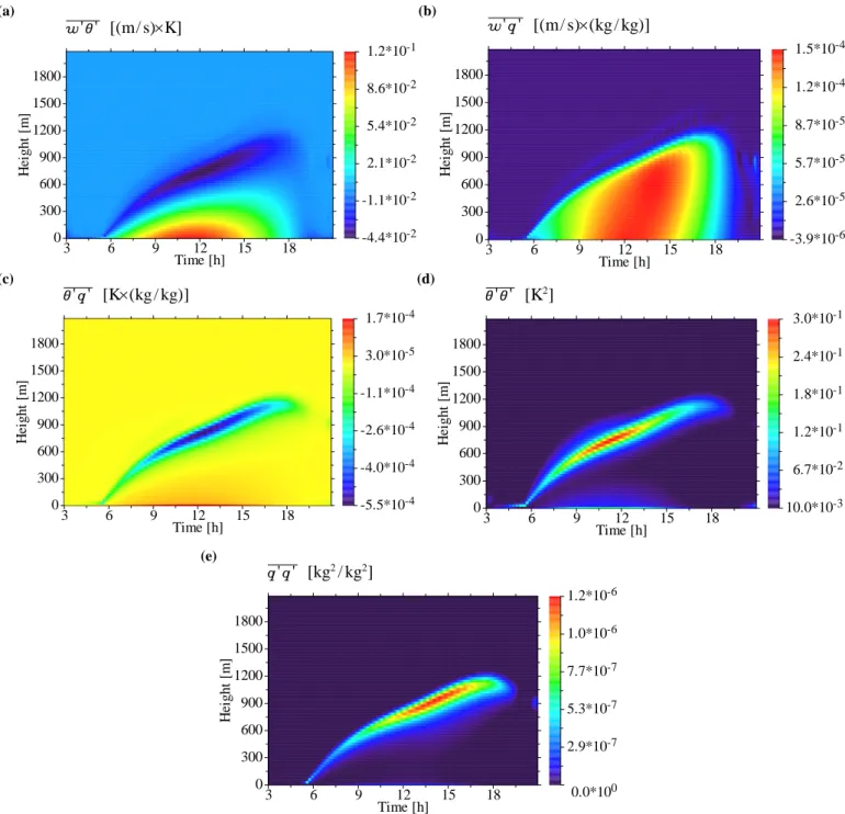
The simulation result of the vertical flux of the water vapour mixing ratio is shown in Fig. 5b.
During the day, the vertical flux of the water vapour mixing ratio attains its maximum around noon, whereas the verti-cal location of that maximum at the surface layer is not that pronounced as for the turbulent heat flux. In the entrainment layer, the turbulent humidity flux is negative. There, spuri-ous oscillations appear, i.e., non-physical solutions result-ing from hyperbolic terms in the governresult-ing equations of the
(a) 3 6 9 12 15 18 Time [h] 0 300 600 900 1200 1500 1800 H ei g h t [m ] -4.4*10-2 -1.1*10-2 2.1*10-2 5.4*10-2 8.6*10-2 1.2*10-1 ' ' [(m/ s) K] (b) 3 6 9 12 15 18 Time [h] 0 300 600 900 1200 1500 1800 H ei g h t [m ] -3.9*10-6 2.6*10-5 5.7*10-5 8.7*10-5 1.2*10-4 1.5*10-4 ' ' [(m/ s) (kg / kg)] (c) 3 6 9 12 15 18 Time [h] 0 300 600 900 1200 1500 1800 H ei g h t [m ] -5.5*10-4 -4.0*10-4 -2.6*10-4 -1.1*10-4 3.0*10-5 1.7*10-4 ' ' [K (kg / kg)] (d) 3 6 9 12 15 18 Time [h] 0 300 600 900 1200 1500 1800 H ei g h t [m ] 10.0*10-3 6.7*10-2 1.2*10-1 1.8*10-1 2.4*10-1 3.0*10-1 ' ' [K2 ] (e) 3 6 9 12 15 18 Time [h] 0 300 600 900 1200 1500 1800 H ei g h t [m ] 0.0*100 2.9*10-7 5.3*10-7 7.7*10-7 1.0*10-6 1.2*10-6 ' ' [kg2 / kg2 ]
Fig. 5. Fluxes and double-correlations of temperature and water vapour mixing ratio: (a) Turbulent vertical flux of potential temperature; (b)
Turbulent vertical flux of water vapour mixing ratio; (c) Co-variance of potential temperature and water vapour mixing ratio; (d) Variance of potential temperature; (e) Variance of water vapour mixing ratio.
third-order moments (see Paper I).
Comparing the humidity flux with LES of the CBL per-formed by Sorbjan (1996a, Fig. 11 for w0q0) and with
obser-vations cited by Verver et al. (1997, Fig. 4 for w0q0, see
ref-erences therein), the humidity flux in the middle CBL seems to be overestimated. However, the humidity flux in Fig. 5b
corresponds well to the result obtained from the third-order turbulence modelling study of the CBL performed by Andr´e et al. (1978, Fig. 5 for w0q0), showing the positive maximum
of the humidity flux occurring just below the MLH. There is a need to evaluate the model with respect to the humid-ity flux prediction. Nevertheless, it is possible to re-adjust
the corresponding parameters in the governing humidity flux equation.
3.3.4 Correlation of potential temperature and water vapour mixing ratio
The predicted time-height cross-section of the correlation of potential temperature and water vapour mixing ratio is pre-sented in Fig. 5c.
The correlation θ0q0assumes positive values in the lower and
negative values in the upper part of the CBL. In the surface layer, positive temperature fluctuations resulting from rising thermals are associated with corresponding positive humidity fluctuations caused, e.g., by humidity sources such as vege-tation or soil moisture. The positive correlation decreases to-ward the entrainment layer, where positive temperature fluc-tuations, resulting from entrainment of potentially warmer air from the stably stratified free troposphere, are associated with negative humidity fluctuations, resulting from the en-trainment of drier free-tropospheric air. Hence, in the entrain-ment layer one has θ0q0<0.
The comparison with previous reference data shows, that the θ0q0behaviour agrees well with the commonly accepted CBL
perception, e.g., of Stull (1997, p. 373, Eq. (9.6.4k)). The simulated co-variance θ0q0 corresponds well to that used
in the model approach of Verver et al. (1997, Fig. 7 for θ0q0). It also agrees well with observational findings cited
therein. Easter and Peters (1994, Fig. 6) investigated the effects of turbulent-scale variations on the binary homoge-neous nucleation rate for correlated and anti-correlated fluc-tuations of temperature and water vapour. Due to the anti-correlation of temperature and humidity fluctuations at the CBL top, the turbulence-enhanced nucleation rate can exceed that at mean-state conditions by a factor of up to 70 (Easter and Peters, 1994).
3.3.5 Variance of potential temperature
Figure 5d shows the simulated evolution of the variance of potential temperature.
The vertical θ0θ0profile reveals two maxima. One maximum
occurs in the surface layer and originates from rising ther-mals in the superadiabatic surface layer. The other one occurs in the entrainment layer originating from overshooting bub-bles penetrating into the stably stratified free troposphere. In the upper third of the well-mixed layer θ0θ0 assumes a
min-imum. During the day, the potential temperature variance is maximal around noon.
The comparison with previous reference data reveals, that the overall behaviour of the potential temperature variance agrees well with that obtained from LES of the CBL per-formed by Sorbjan (1996a, Fig. 9 for θ0θ0), Sorbjan (1996b,
Fig. 6 for θ0θ0), Sullivan et al. (1998, Fig. 5 for θ0θ0) as
well as with that from the second-order turbulence-modelling study of the CBL performed by Abdella and McFarlane
(1997, Fig. 7 for θ0θ0). It also corresponds well to the
semi-empirical profile of the potential temperature variance used in the second-order moment closure study of Verver et al. (1997, Fig. 5 for θ0θ0). Around noon, the Z-shaped θ0θ0
pro-file in Fig. 5d is confirmed by observations of the temperature variance from a wind tunnel study of the CBL performed by Fedorovich et al. (1996, Fig. 9 for T0T0) and by in situ
mea-sured temperature statistics of the CBL provided by Caughey and Palmer (1979, Fig. 5 for θ0θ0).
3.3.6 Humidity variance
The simulation of the time-height cross-section of the humid-ity variance is presented in Fig. 5e.
The evolution of the humidity variance q0q0 exhibits a
pat-tern, which is very similar to that of θ0θ0. Although the
en-hancement of the humidity variance in the surface layer is not as pronounced as that of the temperature variance, there appears also double maxima vertical profile.
The comparison with previous reference data shows, that the general behaviour of the humidity variance is qualita-tively confirmed by the LES studies of the CBL performed by Sorbjan (1996a, Fig. 13 for q0q0), Sorbjan (1996b, Fig. 11
for q0q0) as well as by the semi-empirical profile used in
the second-order moment closure study performed by Verver et al. (1997, Fig. 6 for q0q0). Casadio et al. (1996, Fig. 7
for q0q0) evaluated Raman-LIDAR water vapour
measure-ments in convective plume patterns in the CBL. The ob-served patterns are quite similar to that obtained from the LES studies of Sorbjan (1996a,b), except for the variance in the surface layer. The humidity variance is controlled by the flux partition in the surface layer, hence being a subject of a re-justification of the parameterisation. Very similar to the Raman-LIDAR observations of Casadio et al. (1996) are the water vapour DIAL measurements of absolute humidity vari-ance in the CBL performed by Wulfmeyer (1999a, Fig. 14) and Wulfmeyer (1999b, Fig. 2). As their humidity variance profiles start far above the surface layer, no conclusions about the strength of the surface layer variance maximum predicted by LES can be drawn.
3.4 Third-order moments
3.4.1 Vertical flux of velocity variance
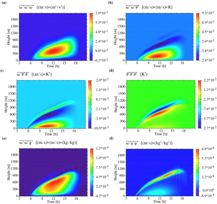
The predicted time-height cross-section of the vertical flux of vertical velocity variance is depicted in Fig. 6a.
The vertical velocity variance flux assumes its maximum around noon in the middle of the CBL. It suddenly decreases in the late afternoon/early evening, when the surface layer buoyancy flux decreases to negative values and the CBL tur-bulence collapses. In the afternoon, the variance flux be-comes negative at the lowest main level, indicating, that the surface acts as a sink for vertical velocity variance.
ver-(a) 3 6 9 12 15 18 Time [h] 0 300 600 900 1200 1500 1800 H ei g h t [m ] -6.3*10-2 9.0*10-2 2.4*10-1 4.0*10-1 5.5*10-1 7.0*10-1 ' ' ' [(m/ s) (m2/ s2)] (b) 3 6 9 12 15 18 Time [h] 0 300 600 900 1200 1500 1800 H ei g h t [m ] -2.8*10-2 -3.8*10-3 2.0*10-2 4.5*10-2 6.9*10-2 9.3*10-2 ' ' ' [(m/ s) (m/ s) K] (c) 3 6 9 12 15 18 Time [h] 0 300 600 900 1200 1500 1800 H ei g h t [m ] -10.0*10-3 -3.9*10-3 2.1*10-3 8.1*10-3 1.4*10-2 2.0*10-2 ' ' ' [(m/ s) K2] (d) 3 6 9 12 15 18 Time [h] 0 300 600 900 1200 1500 1800 H ei g h t [m ] -2.7*10-2 -1.7*10-2 -7.6*10-3 2.3*10-3 1.2*10-2 2.2*10-2 ' ' ' [K3] (e) 3 6 9 12 15 18 Time [h] 0 300 600 900 1200 1500 1800 H ei g h t [m ] -4.2*10-6 2.2*10-5 4.9*10-5 7.5*10-5 1.0*10-4 1.3*10-4 ' ' ' [(m/ s) (m/ s) (kg / kg)] (f) 3 6 9 12 15 18 Time [h] 0 300 600 900 1200 1500 1800 H ei g h t [m ] -8.9*10-9 0.0*100 2.2*10-8 3.7*10-8 5.3*10-8 6.8*10-8 ' ' ' [(m/ s) (kg2/ kg2)]
Fig. 6. Triple correlations of meteorological variables: (a) Flux of vertical wind variance; (b) Flux of turbulent heat flux; (c) Flux of variance
of potential temperature; (d) Third-order moment of potential temperature; (e) Flux of turbulent humidity flux; (f) Flux of variance of water vapour mixing ratio.
tical behaviour of w0w0w0around noon agrees well with the
corresponding profiles obtained from the LES studies of the CBL performed by Moeng and Wyngaard (1988, Fig. 12 for w0w0w0) and Mason (1989, Fig. 9 for w0w0w0) as well as
with those derived from Doppler-SODAR measurements of convective plume patterns in the continental CBL by Casa-dio et al. (1996, Fig. 6 for w0w0w0). A further proof for the
plausibility of the simulated w0w0w0profile is the wind
tun-nel study of a turbulent CBL flow performed by Fedorovich
et al. (1996, Fig. 9b for w0w0w0).
3.4.2 Vertical flux of heat flux
The simulated evolution of the vertical flux of heat flux is shown in Fig. 6b.
The predicted flux of heat flux assumes its maximum in the lower third of the CBL around noon, when turbulence is well-developed. In the entrainment layer, the flux of heat flux is negative. While the heat flux tends to balance out the
tem-perature distribution, the flux of heat flux tends to balance out the heat flux distribution.
The profile of the flux of heat flux around noon agrees well with that derived from LES of the CBL performed by Mo-eng and Wyngaard (1988, Fig. 15 for w0w0θ0) and Sorbjan
(1996b, Fig. 9 for w0w0θ0), furthermore with that used in the
second-order moment closure studies of the CBL carried out by Abdella and McFarlane (1997, Fig. 16 for w0w0θ0), Verver
et al. (1997, Fig. 10 for w0w0θ0) and Zilitinkevich et al. (1999,
Fig. 3 for w0w0θ0).
3.4.3 Vertical flux of temperature variance
Figure 6c shows the simulated time-height cross-section of the vertical flux of temperature variance.
The vertical distribution of w0θ0θ0 reveals a typical S-shape
structure, i.e., a positive maximum near the CBL top, a nega-tive minimum in the entrainment layer, a posinega-tive maximum in the lower quarter of the CBL and a near zero minimum in the surface layer. This S-shape profile is most pronounced when the turbulence is well-developed, i.e., around noon. The vertical profile of w0θ0θ0 is very similar to that
de-rived from LES of the CBL performed by Moeng and Wyn-gaard (1988, Fig. 15 for w0θ0θ0), Sorbjan (1996b, Fig. 10
for w0θ0θ0) as well as to that from second-order moment
clo-sure studies of the CBL performed by Abdella and McFar-lane (1997, Fig. 16 for w0θ0θ0) and Verver et al. (1997, Fig. 9
for w0θ0θ0). Differences between the various profile can be
easily related to corresponding differences of the forcing at lower and upper model boundary (model setup).
3.4.4 Triple correlation of potential temperature
The time-height evolution of the triple correlation of poten-tial temperature is presented in Fig. 6d.
Around noon, the profile of θ0θ0θ0assumes a weak secondary
maximum (>0) in the surface layer, decreasing above to a weak secondary minimum (>0), afterwards increasing again to assume an absolute maximum just below the CBL top and decreasing above to an absolute minimum (<0) in the en-trainment layer.
This profile is in qualitatively good agreement with previ-ous results from the LES of the CBL performed by Sorbjan (1996a, Fig. 10 for θ0θ0θ0) and from the second-order
mo-ment closure study of the CBL performed by Verver et al. (1997, Fig. 8 for θ0θ0θ0). Observed differences in the
en-trainment layer (θ0θ0θ0≤0 in Fig. 10 of Sorbjan (1996a) and
(θ0θ0θ0>0 in Fig. 8 of Verver et al., 1997) are due to the
dif-ferent strength of the CBL top inversion. 3.4.5 Vertical flux of humidity flux
Figure 6e shows the evolution pattern of the vertical flux of humidity flux.
For this simulation and for the following triple correlations,
no profiles from previous LES, wind tunnel or CBL observa-tional studies could be found for comparison.
The vertical flux of humidity flux is nearly almost greater than zero, i.e., a downward directed humidity flux is down-ward transported by CBL turbulence, an updown-ward directed hu-midity flux is upward transported. The flux of huhu-midity flux assumes its maximum in the upper third of the CBL. It tends to well-mix the humidity flux throughout the CBL. Negative values occur in the entrainment layer. The vertical stripes, pe-riodically appearing in the afternoon entrainment layer, are resulting from non-physical spurious oscillations, that were not fully damped.
3.4.6 Vertical flux of humidity variance
The vertical flux of humidity variance in Fig. 6f assumes a weak positive maximum in the lowest quarter of the CBL and a pronounced one in the entrainment layer. The low-level maximum results from upward transport of enhanced humid-ity variance in the surface layer by buoyant eddies. The max-imum in the entrainment layer results from upward transport of enhanced humidity variance by large eddies penetrating into the free troposphere.
3.4.7 Vertical flux of potential temperature/water vapour mixing ratio correlation
The flux of temperature–humidity correlation, depicted in Fig. 7a, is positive throughout the CBL except for the en-trainment layer, where it assumes negative values. Due to the commutativity of variables in cross-correlation terms, the flux of double correlation can be interpreted as a double cor-relation between the vertical component of the turbulent heat flux and the water vapour mixing ratio. Thus, in the lower third of the CBL the turbulent heat flux is positively corre-lated with the water vapour mixing ratio, i.e., the upward-directed turbulent heat flux, originated in the surface layer, is associated with positive humidity fluctuations. In the en-trainment layer both terms are anti-correlated. There, buoy-ant eddies penetrating into the free troposphere (w0>0) are correlated with positive fluctuations of the potential temper-ature, originating from entrainment of potentially warmer free-tropospheric air (θ0>0), and with negative fluctuations of the water vapour mixing ratio, originating from entrain-ment of drier free-tropospheric air (q0<0). This results in a pronounced negative minimum of w0θ0q0 in the entrainment
layer.
3.4.8 Correlation of potential temperature variance and wa-ter vapour mixing ratio as well as correlation of wawa-ter vapour mixing ratio variance and potential tempera-ture
The triple correlations θ0θ0q0 (Fig. 7b) and θ0q0q0 (Fig. 7c)
(a) 3 6 9 12 15 18 Time [h] 0 300 600 900 1200 1500 1800 H ei g h t [m ] -2.2*10-5 -1.2*10-5 -2.5*10-6 7.1*10-6 1.7*10-5 2.6*10-5 ' ' ' [(m/ s) K (kg / kg)] (b) 3 6 9 12 15 18 Time [h] 0 300 600 900 1200 1500 1800 H ei g h t [m ] -3.7*10-5 -1.7*10-5 3.2*10-6 2.3*10-5 4.3*10-5 6.3*10-5 ' ' ' [K2 (kg / kg)] (c) 3 6 9 12 15 18 Time [h] 0 300 600 900 1200 1500 1800 H ei g h t [m ] -1.5*10-7 -1.1*10-7 -6.3*10-8 0.0*100 2.6*10-8 7.1*10-8 ' ' ' [K (kg2/ kg2)] (d) 3 6 9 12 15 18 Time [h] 0 300 600 900 1200 1500 1800 H ei g h t [m ] -1.5*10-10 0.0*100 8.0*10-11 2.0*10-10 3.1*10-10 4.3*10-10 ' ' ' [kg3 / kg3 ]
Fig. 7. Triple correlations of temperature and humidity: (a) Flux of co-variance of potential temperature and water vapour mixing ratio; (b)
Correlation of temperature variance and humidity; (c) Correlation of temperature and humidity variance; (d) Third-order moment of water vapour mixing ratio.
CBL. Just below the CBL top, entrainment of poten-tially warmer free-tropospheric air (θ0>0) is associated
with temperature–humidity anti-correlation (θ0q0<0)
result-ing in θ0θ0q0<0. Just above, detrainment of potentially
colder CBL air (θ0<0) leads to θ0θ0q0>0. For θ0q0q0 the
conditions are reversed. Just below the CBL top, entrain-ment of drier free-tropospheric air (q0<0) is associated with temperature–humidity anti-correlation (θ0q0<0) resulting in
θ0q0q0>0. Just above, the detrainment of moister CBL air
(q0>0) results in θ0q0q0<0.
3.4.9 Triple correlation of water vapour mixing ratio The double-peak structure in the entrainment layer can also be seen in the q0q0q0 profile shown in Fig. 7d. Just below
the CBL top q0q0q0becomes lower, just above the CBL top
greater than zero. The strength of the double-peak pattern in the entrainment layer profiles of θ0θ0θ0 (Fig. 6d), θ0θ0q0
(Fig. 7b), θ0q0q0(Fig. 7c) and q0q0q0(Fig. 7d) is directly
re-lated to the strength of the capping inversion. The modelling of second-order and third-order moments just there deserves further tuning of the parameterisation and, perhaps, of the numerical scheme. For fine-tuning, additional reference data
of third-order moments derived from LES, wind tunnel stud-ies and/or in situ observations are necessary.
3.5 Surface layer properties
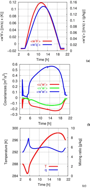
The turbulent vertical fluxes of sensible heat, latent heat and momentum in the surface layer are depicted in Figs. 8a–c. At night, the turbulent heat flux is negative, i.e., directed toward the surface (Fig. 8a, red curve). After sunrise it in-creases, assuming its maximum around noon.
The humidity flux is negative at night, i.e., deposition of hu-midity occurs (dew) (Fig. 8a, blue curve). When the sun el-evates above the horizon, a part of the incoming solar radia-tion contributes to evaporaradia-tion, leading to an increase of the humidity flux synchronously to the diurnal variation of the sensible heat flux (Holtslag, 1987, p. 23–46) (surface layer parameterisation, see Paper I, Subsubsection 5.2.1 and Ap-pendix D2.2).
The variance of the vertical velocity in the surface layer is shown in Fig. 8b (blue curve). The sharp drop of the initial value of w0w0 at the beginning is related to the adaptation
phase of the model. Afterwards, w0w0increases in the course
when CBL turbulence is well-developed. The vertical fluxes of the horizontal wind components in the surface layer, w0u0
and w0v0, are negative, i.e., owing to aerodynamic roughness
the surface acts as a sink for the momentum flux.
The temperature and humidity evolution in the course of the day are shown in Fig. 8c. The temperature minimum and the maximum of the water vapour mixing ratio coin-cide and appear just before sunrise. Afterwards, the air tem-perature in the surface layer rises due to increasing flux of sensible heat. The rise of water vapour mixing ratio during the day due to increasing humidity flux is superimposed by turbulence-induced dilution. This results in a weak secondary maximum of q around noon.
4 Summary and conclusion
Simulated first-, second- and third-order moments of the CBL agree well with previous results from LES and wind tunnel studies as well with with available in situ observations and remote sensing data. Doppler-SODAR, RADAR-RASS and water vapour DIAL provide a high potential of infor-mation for the evaluation of second-order moments. Differ-ences in the behaviour of some third-order moments near the entrainment layer can be related to differences in the strength of the CBL top inversion. With respect to these dif-ferences it should be noted, that one part of the reference data directly confirms the present simulations, another does not. Hence, further investigations are deserved to calibrate the model. High-order moments, for which no comparative reference results are available, show a physically plausible behaviour. Altogether, the simulation performed here is a suitable base to study NPF in the CBL, especially to exam-ine previous hypotheses on the role of turbulence in the evo-lution of NPF bursts. As the non-reactive part of the chem-ical and aerosoldynamchem-ical model equations are technchem-ically and per algorithm identical to the governing equations for the second-order and third-order moments of meteorological variables, the conducted model examination for meteorolog-ical flow properties may serve, to some degree, as a control for the computational feasibility of third-order modelling of both physicochemical and aerosoldynamical properties. Nev-ertheless, the turbulence model deserves further fine-tuning, explicit verification/validation and model inter-comparison studies using high-order moments, that are both directly de-rived from in situ observations and indirectly dede-rived from remote sensing. Based on the CBL simulation presented here, in the subsequent Paper III a conceptual study on NPF in the anthropogenically influenced CBL will be performed. In Pa-per IV, the results will be discussed and compared with a number of in situ measurements of NPF under very different conditions to verify or falsify, respectively, a state-of-the-art hypothesis on the role of turbulence in NPF.
−0.02 0 0.02 0.04 0.06 0.08 0.1 0.12 2 6 10 14 18 22 0 0.02 0.04 0.06 0.08 0.1 0.12 0.14 0.16 <w’ θ ’> [(m/s) x (K)] <w’q’> [(m/s) x (g/kg)] Time [h] <w’θ’> <w’q’> (a) −0.3 −0.2 −0.1 0 0.1 0.2 0.3 0.4 0.5 0.6 2 6 10 14 18 22 Covariances [m 2 /s 2 ] Time [h] <u’w’> <v’w’> <w’w’> (b) 284 288 292 296 300 2 6 10 14 18 22 0 2 4 6 8 10
Temperature [K] Mixing ratio [g/kg]
Time [h]
T
q
(c)
Fig. 8. Time series of meteorological variables in the surface layer: (a) Turbulent heat and humidity flux; (b) Turbulent moment fluxes; (c) Temperature and water vapour mixing ratio.
Acknowledgements. The work was realised at the IfT Modelling Department headed by E. Renner within the framework of IfT main research direction 1 “Evolution, transport and spatio-temporal distribution of the tropospheric aerosol”. For the motivation and numerous discussions on the subject of the present Paper I am very indebted to D. Mironov, E. Renner, K. Bernhardt, E. Schaller, M. Kulmala, A. A. Lushnikov, M. Boy, R. Wolke, F. Stratmann, H. Siebert, T. Berndt and J. W. P. Schmelzer. Sincerest thanks are given to M. Kulmala and M. Boy for the opportunity to present
and discuss previous results at the Department of Physics at the University of Helsinki. Many thanks go to the editor and to the three reviewers for their helpful comments and suggestions to improve the manuscript. Special thanks go also to N. Otto and N. Deisel for their strong support during the technical processing as well as to M. Reichelt for the proofreading of the manuscript. Edited by: M. Kulmala
References
Aalto, P., H¨ameri, K., Becker, E., Weber, R., Salm, J., M¨akel¨a, J. M., Hoell, C., O’Dowd, C. D., Karlsson, H., Hansson, H.-C., V¨akev¨a, M., Koponen, I. K., Buzorius, G., and Kulmala, M.: Physical characterization of aerosol particles during nucleation events, Tellus, 53B, 344–358, 2001.
Abdella, K. and McFarlane, N.: A new second-order turbulence closure scheme for the planetary boundary layer, J. Atmos. Sci., 54, 1850–1867, 1997.
Andr´e, J. C., De Moor, G., Lacarr`ere, P., Therry, G., and Du Vachat, R.: Modeling the 24-hour evolution of the mean and turbulent structures of the planetary boundary layer, J. Atmos. Sci., 35, 1861–1883, 1978.
Birmili, W. and Wiedensohler, A.: New particle formation in the continental boundary layer: Meteorological and gas phase parameter influence, Geophys. Res. Lett., 27(20), 3325–3328, 2000.
Birmili, W., Wiedensohler, A., Plass-D¨ulmer, C., and Berresheim, H.: Evolution of newly formed aerosol particles in the continen-tal boundary layer: A case study including OH and H2SO4
mea-surements, Geophys. Res. Lett., 27(15), 2205–2208, 2000. Birmili, W., Berresheim, H., Plass-D¨ulmer, C., Elste, T., Gilge,
S., Wiedensohler, A., and Uhrner, U.: The Hohenpeissenberg aerosol formation experiment (HAFEX): A long-term study in-cluding size-resolved aerosol, H2SO4, OH, and monoterpenes
measurements, Atmos. Chem. Phys., 3, 361–376, 2003, http://www.atmos-chem-phys.net/3/361/2003/.
Bonn, B. and Moortgat, G. K.: New particle formation during α-and β-pinene oxidation by O3, OH and NO3, and the influence
of water vapour: Particle size distribution studies, Atmos. Chem. Phys., 2, 183–196, 2002,
http://www.atmos-chem-phys.net/2/183/2002/.
Bonn, B. and Moortgat, G. K.: Sesquiterpene ozonolysis: Origin of atmospheric new particle formation from biogenic hydrocarbons, Geophys. Res. Lett., 30(11), 1585, doi:10.1029/2003GL017000, 2003.
Bonn, B., Schuster, G., and Moortgat, G. K.: Influence of water va-por on the process of new particle formation during monoterpene ozonolysis, J. Phys. Chem. A, 106, 2869–2881, 2002.
Bonn, B., v. Kuhlmann, R., and Lawrence, M. G.: High contribution of biogenic hydroperoxides to secondary or-ganic aerosol formation, Geophys. Res. Lett., 31, L10108, doi:10.1029/2003GL019172, 2004.
Boy, M.: Nucleation events in the continental planetary boundary layer – physical, chemical and meteorological influences, Re-port Series in Aerosol Science, No. 60, Division of Atmospheric Sciences, Department of Physical Sciences, Faculty of Sciences, University of Helsinki, Finland, academic dissertation, 2003.
Boy, M. and Kulmala, M.: Nucleation events in the continental boundary layer: Influence of physical and meteorological param-eters, Atmos. Chem. Phys., 2, 1–16, 2002,
http://www.atmos-chem-phys.net/2/1/2002/.
Boy, M., Rannik, ¨U., Lehtinen, K. E. J., Tarvainen, V., Hakola, H., and Kulmala, M.: Nucleation events in the continen-tal boundary layer: Long-term statistical analyses of aerosol relevant characteristics, J. Geophys. Res., 108(D21), 4667, doi:10.1029/2003JD003838, 2003.
Boy, M., Pet¨aj¨a, T., Dal Maso, M., Rannik, ¨U., Rinne, J., Aalto, P., Laaksonen, A., Vaattovaara, P., Joutsensaari, J., Hoffmann, T., Warnke, J., Apostolaki, M., Stephanou, E. G., Tsapakis, M., Kouvarakis, A., Pio, C., Carvalho, A., R¨ompp, A., Moortgat, G., Spirig, C., Guenther, A., Greenberg, J., Ciccioli, P., and Kulmala, M.: Overview of the field measurement campaign in Hyyti¨al¨a, August 2001 in the framework of the EU project OSOA, Atmos. Chem. Phys., 4, 657–678, 2004,
http://www.atmos-chem-phys.net/4/657/2004/.
Buzorius, G., Rannik, ¨U., Nilsson, D., and Kulmala, M.: Vertical fluxes and micrometeorology during aerosol particle formation events, Tellus, 53B, 394–405, 2001.
Buzorius, G., Rannik, ¨U., Aalto, P., dal Maso, M., Nilsson, E. D., Lehtinen, K. E. J., and Kulmala, M.: On particle formation prediction in continental boreal forest using micro-meteorological parameters, J. Geophys. Res., 108(D13), 4377, doi:10.1029/2002JD002850, 2003.
Casadio, S., Di Sarra, A., Fiocco, G., Fu`a, D., Lena, F., and Rao, M. P.: Convective characteristics of the nocturnal urban boundary layer as observed with Doppler sodar and Raman li-dar, Boundary-Layer Meteorol., 79, 375–391, 1996.
Caughey, S. J. and Palmer, S. G.: Some aspects of turbulence struc-ture through the depth of the convective boundary layer, Quart. J. Roy. Meteorol. Soc., 105, 811–827, 1979.
Clement, C. F. and Ford, I. J.: Gas-to-particle conversion in the atmosphere: I. Evidence from empirical atmospheric aerosols, Atmos. Environ., 33, 475–487, 1999.
Clement, C. F., Pirjola, L., dal Maso, M., M¨akel¨a, J. M., and Kul-mala, M.: Analysis of particle formation bursts observed in Fin-land, J. Aerosol Sci., 32, 217–236, 2001.
Coe, H., Williams, P. I., McFiggans, G., Gallagher, M. W., Beswick, K. M., Bower, K. N., and Choularton, T. W.: Behavior of ultra-fine particles in continental and marine air masses at a rural site in the United Kingdom, J. Geophys. Res., 105(D22), 26 891– 26 905, 2000.
Cohn, S. A. and Angevine, W. M.: Boundary layer height and en-trainment zone thickness measured by Lidars and wind-profiling Radars, J. Appl. Meteorol., 39, 1233–1247, 2000.
Cuijpers, J. W. M. and Holtslag, A. A. M.: Impact of skewness and nonlocal effects on scalar and buoyancy fluxes in convective boundary layers, J. Atmos. Sci., 55, 151–162, 1998.
Dal Maso, M., Kulmala, M., Riipinen, I., Wagner, R., Hussein, T., Aalto, P. P., and Lehtinen, K. E. J.: Formation and growth of fresh atmospheric aerosols: Eight years of aerosol size distribu-tion data from SMEAR II, Hyyti¨al¨a, Finland, Boreal Environ. Res., 10, 323–336, 2005.
Easter, R. C. and Peters, L. K.: Binary homogeneous nucleation: Temperature and relative humidity fluctuations, nonlinearity, and aspects of new particle production in the atmosphere, J. Appl. Meteorol., 33, 775–784, 1994.
Fedorovich, E., Kaiser, R., Rau, M., and Plate, E.: Wind tunnel study of turbulent flow structure in the convective boundary layer capped by a temperature inversion, J. Atmos. Sci., 53, 1273– 1289, 1996.
Garratt, J. R.: The Atmospheric Boundary Layer, Cambridge atmo-spheric and space science series, Cambridge University Press, Cambridge, United Kingdom, 1992.
Gaydos, T. M., Stanier, C. O., and Pandis, S. N.: Mod-eling of in situ ultrafine atmospheric particle formation in the eastern United States, J. Geophys. Res., 110, D07S12, doi:10.1029/2004JD004683, 2005.
Gerrity Jr., J. P.: Modeling the planetary boundary layer: Fric-tional influence, Office Note 131, U.S. Department of Com-merce, National Oceanic and Atmospheric Administration, Na-tional Weather Service, NaNa-tional Meteorological Center, Devel-opment Division, 1976.
Held, A., Nowak, A., Birmili, W., Wiedensohler, A., Forkel, R., and Klemm, O.: Observations of particle formation and growth in a mountainous forest region in central Europe, J. Geophys. Res., 109, D23204, doi:10.1029/2004JD005346, 2004.
Hess, G. D.: Parameterisation of the atmospheric boundary layer: A retrospective look, 16th BMRC Modelling Workshop 2004, Bureau of Meteorology Research Centre, Melbourne, Australia, 2004.
Holtslag, A. A. M.: Surface fluxes and boundary layer scal-ing. Models and applications, Scientific Report WR 87-2(FM), Koninklijk Nederlands Meteorologisch Instituut, De Bilt, 1987. Hyv¨onen, S., Junninen, H., Laakso, L., Dal Maso, M., Gr¨onholm,
T., Bonn, B., Keronen, P., Aalto, P., Hiltunen, V., Pohja, T., Lau-niainen, S., Hari, P., Mannila, H., and Kulmala, M.: A look at aerosol formation using data mining techniques, Atmos. Chem. Phys., 5, 3345–3356, 2005,
http://www.atmos-chem-phys.net/5/3345/2005/.
Kulmala, M.: How particles nucleate and grow, Science, 302, 1000– 1001, 2003.
Kulmala, M., Toivonen, A., M¨akel¨a, J. M., and Laaksonen, A.: Analysis of the growth of nucleation mode particles observed in boreal forest, Tellus, 50B, 449–462, 1998.
Kulmala, M., Dal Maso, M., M¨akel¨a, J. M., Pirjola, L., V¨akev¨a, M., Aalto, P., Miikkulainen, P., H¨ameri, K., and O’Dowd, C. D.: On the formation, growth and composition of nucleation mode particles, Tellus, 53B, 479–490, 2001a.
Kulmala, M., H¨ameri, K., Aalto, P. P., M¨akel¨a, J. M., Pirjola, L., Nilsson, E. D., Buzorius, G., Rannik, ¨U., Dal Maso, M., Seidl, W., Hoffman, T., Janson, R., Hansson, H.-C., Viisanen, Y., Laak-sonen, A., and O’Dowd, C. D.: Overview of the international project on biogenic aerosol formation in the boreal forest (BIO-FOR), Tellus, 53B, 324–343, 2001b.
Kulmala, M., Laakso, L., Lehtinen, K. E. J., Riipinen, I., Dal Maso, M., Anttila, T., Kerminen, V.-M., H˜orrak, U., Vana, M., and Tam-met, H.: Initial steps of aerosol growth, Atmos. Chem. Phys., 4, 2553–2560, 2004a.
Kulmala, M., Vehkam¨aki, H., Pet¨aj¨a, T., Dal Maso, M., Lauri, A., Kerminen, V.-M., Birmili, W., and McMurry, P. H.: Formation and growth rates of ultrafine atmospheric particles: A review of observations, J. Aerosol Sci., 35, 143–176, 2004b.
Kulmala, M., Lehtinen, K. E. J., Laakso, L., Mordas, G., and H¨ameri, K.: On the existence of neutral atmospheric clusters, Boreal Environ. Res., 10, 79–87, 2005.
Mason, P. J.: Large-eddy simulation of the convective atmospheric boundary layer, J. Atmos. Sci., 46, 1492–1516, 1989.
Moeng, C.-H. and Wyngaard, J. C.: Spectral analysis of large-eddy simulations of the convective boundary layer, J. Atmos. Sci., 45, 3573–3587, 1988.
Monin, A. S. and Obuchow, A. M.: Fundamentale Gesetzm¨aßigkeiten der turbulenten Vermischung in der bo-dennahen Schicht der Atmosph¨are, in: Sammelband zur statistischen Theorie der Turbulenz, mit Beitr¨agen von A. N. Kolmogorov, A. M. Obuchow, A. M. Jaglom, A. S. Monin, edited by Goering, H., pp. 199–228, Deutsche Akademie der Wissenschaften zu Berlin, Akademie-Verlag, Berlin, 1958. Monin, A. S. and Obukhov, A. M.: Basic laws of turbulent
mix-ing in the atmosphere near the ground, reprinted from Trudy, Akademiia Nauk SSSR, Geofizicheskogo Instituta, Vol. 24(151), 163–187 (1954), in: Selected Papers on Turbulence in a Refrac-tive Medium, edited by Andreas, E. L., SPIE Milestone Series, Volume MS 25, pp. 300–312, SPIE Optical Engineering Press, 1990.
Muschinski, A., Sullivan, P. P., Wuertz, D. B., Hill, R. J., Cohn, S. A., Lenschow, D. H., and Doviak, R. J.: First synthesis of wind-profiler signals on the basis of large-eddy simulation data, Radio Science, 34, 1437–1459, 1999.
Nilsson, E. D., Rannik, ¨U., Paatero, J., Boy, M., O’Dowd, C., Bu-zorius, G., Laakso, L., and Kulmala, M.: Effects of synoptic weather and boundary layer dynamics on aerosol formation in the continental boundary layer, in: Abstracts of the European Aerosol Conference 2000, vol. 31, suppl. 1 of J. Aerosol Sci., pp. S600–S601, Pergamon, 2000.
Nilsson, E. D., Paatero, J., and Boy, M.: Effects of air masses and synoptic weather on aerosol formation in the continental bound-ary layer, Tellus, 53B, 462–478, 2001a.
Nilsson, E. D., Rannik, ¨U., Kulmala, M., Buzorius, G., and O’Dowd, C. D.: Effects of continental boundary layer evolution, convection, turbulence and entrainment, on aerosol formation, Tellus, 53B, 441–461, 2001b.
O’Dowd, C. D., Aalto, P. P., Yoon, Y. J., and H¨ameri, K.: The use of the pulse height analyser ultrafine condensation particle counter (PHA-UCPC) technique applied to sizing of nucleation mode particles of differing chemical composition, J. Aerosol Sci., 35, 205–216, 2004.
Prandtl, L.: ¨Uber die Fl¨ussigkeitsbewegung bei sehr kleiner Rei-bung, in: Verhandlgn. d. III. Intern. Math. Kongr., Heidelberg, 8.-13. August 1904, pp. 485–491, B. G. Teubner Verlag, Leipzig, 1905.
Prandtl, L.: Bericht ¨uber Untersuchungen zur ausgebildeten Turbu-lenz, Z. angew. Math. Mech., 5, 136–139, 1925.
Siebert, H., Stratmann, F., and Wehner, B.: First observations of in-creased ultrafine particle number concentrations near the inver-sion of a continental planetary boundary layer and its relation to ground-based measurements, Geophys. Res. Lett., 31, L09102, doi:10.1029/2003GL019086, 2004.
Sorbjan, Z.: Numerical study of penetrative and “solid lid” nonpen-etrative convective boundary layers, J. Atmos. Sci., 53, 101–112, 1996a.
Sorbjan, Z.: Effects caused by varying the strength of the capping inversion based on a large eddy simulation model of the shear-free convective boundary layer, J. Atmos. Sci., 53, 2015–2024, 1996b.
Steinbrecher, R. and the BEWA2000-Team: Regional biogenic emissions of reactive volatile organic compounds (BVOC) from forests: Process studies, modelling and validation experiments (BEWA2000), AFO2000-Newsletter, 8(9-2004), 7–10, unpub-lished manuscript, 2004.
Stratmann, F., Siebert, H., Spindler, G., Wehner, B., Althausen, D., Heintzenberg, J., Hellmuth, O., Rinke, R., Schmieder, U., Sei-del, C., Tuch, T., Uhrner, U., Wiedensohler, A., Wandinger, U., Wendisch, M., Schell, D., and Stohl, A.: New-particle forma-tion events in a continental boundary layer: First results from the SATURN experiment, Atmos. Chem. Phys., 3, 1445–1459, 2003,
http://www.atmos-chem-phys.net/3/1445/2003/.
Stull, R. B.: An Introduction to Boundary Layer Meteorology, Kluwer Academic Publishers, Dordrecht, 1997.
Sullivan, P. P., McWilliams, J. C., and Moeng, C.-H.: A grid nesting method for large-eddy simulation of planetary boundary-layer flows, Boundary-Layer Meteorol., 80, 167–202, 1996.
Sullivan, P. P., Moeng, C.-H., Stevens, B., Lenschow, D. H., and Mayor, S. D.: Structure of the entrainment zone capping the con-vective atmospheric boundary layer, J. Atmos. Sci., 55, 3042– 3064, 1998.
Turner, J. S.: Buoyancy Effects in Fluids, Cambridge University Press, 1973.
Uhrner, U., Birmili, W., Stratmann, F., Wilck, M., Ackermann, I. J., and Berresheim, H.: Particle formation at a continental back-ground site: Comparison of model results with observations, At-mos. Chem. Phys., 3, 347–359, 2003,
http://www.atmos-chem-phys.net/3/347/2003/.
Verver, G. H. L., van Dop, H., and Holtslag, A. A. M.: Turbu-lent mixing of reactive gases in the convective boundary layer, Boundary-Layer Meteorol., 85, 197–222, 1997.
Wulfmeyer, V.: Investigation of turbulent processes in the lower troposphere with water vapor DIAL and radar-RASS, J. Atmos. Sci., 56, 1055–1076, 1999a.
Wulfmeyer, V.: Investigations of humidity skewness and variance profiles in the convective boundary layer and comparison of the latter with large eddy simulation results, J. Atmos. Sci., 56, 1077–1087, 1999b.
Zilitinkevich, S., Gryanik, V. M., Lykossov, V. N., and Mironov, D. V.: Third-order transport and nonlocal turbulence closures for convective boundary layers, J. Atmos. Sci., 56, 3463–3477, 1999.