Ranking and selecting association rules based on dominance relationship

HAL Id: hal-00677853

https://hal.archives-ouvertes.fr/hal-00677853

Preprint submitted on 24 May 2012

HAL is a multi-disciplinary open access

archive for the deposit and dissemination of

sci-entific research documents, whether they are

pub-lished or not. The documents may come from

teaching and research institutions in France or

abroad, or from public or private research centers.

L’archive ouverte pluridisciplinaire HAL, est

destinée au dépôt et à la diffusion de documents

scientifiques de niveau recherche, publiés ou non,

émanant des établissements d’enseignement et de

recherche français ou étrangers, des laboratoires

publics ou privés.

Ranking and selecting association rules based on

dominance relationship

Slim Bouker

To cite this version:

Slim Bouker. Ranking and selecting association rules based on dominance relationship. 2012.

�hal-00677853�

Ranking and selecting association rules based on

dominance relationship

Slim Bouker and Rabie Saidi and Sadok Ben Yahia and Engelbert Mephu Nguifo

Abstract. The huge number of association rules represent the main obstacle that a decision maker faces. In order to bypass this obstacle, an efficient selection of rules must be performed. Since selection is necessarily based on evaluation, many interestingness measures have been proposed. However, the abundance of these measures caused a new problem which is the heterogeneity of the evaluation results and this created confusion to the decision. In this scope, we propose a novel approach to discover interesting association rules without favouring or excluding any measure by adopting the notion of dom-inance between rules. Our approach bypasses the problem of mea-sure heterogeneity and find a compromise between their evaluations and also bypasses another non-trivial problem which is the threshold value specification.

1

INTRODUCTION

Mining association rules is one of the core tasks in data mining re-search. Since its first formalization in [1], the research on association rules has become very popular among the data mining researchers, as it provides an opportunity to extract relevant and valuable relation-ship between attributes in transaction databases.

At present, association rules are widely used in the decision

making related to various areas such as telecommunication net-works, market and risk management, inventory control etc, where the databases are generally large [13]. However, it is well known that data mining algorithms produce huge numbers of rules [8]. Hence, the decision maker is unable to determine the most interesting ones and consequently unable to make decisions. In order to face this ob-stacle, an efficient evaluation of rules has become a need rather than being a rational choice. Several works have been devoted to study the interestingness of association rules [6], [7], [17], [19]. As a con-sequence, a panoply of statistical measures, obeying different seman-tics, have been proposed. Although these measures allow evaluating rules from various sights, yet their abundance (≈ 60) has yielded an-other problem for the decision maker. Indeed, the outputs of evalua-tions vary from a measure to another and may even be contradictory since the measures evaluate differently the rules under consideration. That is why, it is common that a given rule be considered relevant according to a measure and irrelevant according to another.

The problem caused by the abundance of measures has led to a trend of works that focuss on proposing approaches to assist the user(i.e., the decision maker) in selecting the measures qualified to be the most adequate to the decision scope. These approaches can be classified into two main categories namely the expert-based

ap-1_{Clermont Universit, Universit Blaise Pascal, LIMOS, BP 10448, F-63000}

CLERMONT-FERRAND, email: slim.bouker@isima.fr, saidi@isima.fr, sadok.benyahia@fst.rnu.tn, mephu@isima.fr

proaches and the property-based approaches. In the first category, different studies have compared the ranking of rules by human ex-perts to the ranking of rules by various measures. Then, they sug-gested choosing the measure that produces the ranking which most resembles the expert one [15], [18]. These studies were based on specific datasets and experts. Thus, their results cannot be taken as general conclusions. Moreover, in a real problem, it is not always possible to get rule ranking by experts. As for the second category, to reduce the number of measures, many properties have been reported in [4]. Geng and Hamilton surveyed the interestingness of measures and summarized nine properties to address that issue. Using proper-ties facilitates a general and practical way to automatically identify interesting measures. This trend has been enriched by different other works [2], [5], [11], [12] with an extensive number of properties. Nevertheless, these properties are not standards [10]. Hence, they do not guarantee selecting only one best measure. Indeed, a wide range of UCI2datasets were also used to study the impact of different prop-erties. The results show no single measure can be introduced as an obvious winner [5]. Then, in the case of selecting many measures, the problem related to the variety of outputs, mentioned above, persists. In other words, the user cannot proceed towards a unique selection of rules. Whatever one measure is selected or more, nothing guarantees that they are the ”best” ones and some better suited measures may be excluded for the simple reason that the used properties do not take into account the specificity of decision context.

Our contribution lies within this scope. In this paper, we propose a novel approach to discover interesting association rules without fa-voring or excluding any mesure among the used measures. For this purpose, we integrate into the rule selection process, the skyline

op-erator[3] whose fundamental principle relies on the notion of

dom-inance. Skyline operator is used to resolve mathematical and eco-nomics problems such as maximum vectors [9], Pareto set [14] and multi-objective optimization [16]. In our work, the skyline operator comprises the rules that are supposed to be the most interesting ones while taking into account several measures. The dominance relation-ship which is the corner stone of the skyline operator is applied on rules and can be presented as follows: a rule r is said dominated by another rule r′, if for all used measures, r is less relevant than r′. The former rule (i.e., r) is discarded from the result, not because it is not relevant for one of the mesure but because it is not interesting ac-cording to the combination of all measures. Our approach bypasses the problem of measure selection by finding a compromise between the different outputs and also bypasses another nontrivial problem which is the threshold value specification.

The remainder of this paper is organized as follows. Section 2 gives a brief definitions related to association rules and introduce

the dominance relationship. We propose and detail our approach of rule selection in section 3. An extension of our approach to enable rule ranking is presented in section 4. Concluding points and some prospectives make the body of section 5.

2

ASSOCIATION RULES AND DOMINANCE

RELATIONSHIP

In this section we first recall basic definitions related to association rules. Then, we present these rules as numeric vectors within the same dimension after having been evaluated by a set of measures. This vector format, allows us to benefit from the concept of

domi-nanceand adapt it to our scope as described in section 2.2.

2.1

Association rules

LetI be a set of literal called items, an itemset corresponds to a non null subset ofI. These itemsets are gathered together in the set L :L = 2I_{\∅. In a transactional dataset, each transaction contains an}

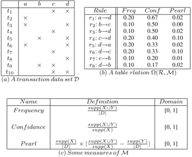
itemset ofL. Table 1(a) presents a transactional dataset D where 10 transactions denoted by t1, . . . , t10are described by 4 items denoted

by a, b, c, d. The support of an itemset X, denoted supp(X), is the number of transactions containing X. The negative support supp(X) is the number of transactions that do not contain X.

An association rule r is a relation between itemsets of the form r: X→Y where X and Y are itemsets, and X∩Y =∅. Itemsets X and Y are called, respectively, premise and conclusion of r. The support of r is equal to the number of transactions containing both X and Y , supp(r)= supp(X∪Y). We notice that interesting measures for asso-ciation rules are usually defined using support counts as presented in Table1(b). a b c d t1 × × t2 × t3 × × t4 × t5 × × t6 × × t7 × t8 × t9 × × t10 × ×

(a) A transaction data set D

Rule F req Conf P earl r1: a→d 0.20 0.67 0.02 r2: b→c 0.10 0.50 0.00 r3: b→d 0.10 0.50 0.02 r4: c→d 0.20 0.40 0.10 r5: d→a 0.20 0.33 0.02 r6: d→c 0.20 0.33 0.10 r7: c→b 0.10 0.20 0.01 r8: d→b 0.10 0.17 0.02 (b) A table rlation Ω(R, M)

N ame Def inition Domain

F requency supp(X∪Y )_|D| [0, 1] Conf idance supp(X∪Y )_supp(X) [0, 1] P earl supp(X)_|D| × |supp(X∪Y )_supp(X) −supp(Y )_|D| | [0, 1]

(c) Some measures of M

Table 1. Example of a dataset transaction and measures.

2.2

Dominance relationship

After mining association rules from transactional dataset D (e.g., Table1(a)), a setR of rules is obtained (e.g., Table1(b) first column).

Rules ofR are evaluated by a set M of measures (e.g., Table1(c)) to form a relational tableΩ (e.g., Table1(b)). Formally, Ω = (R,M) with the setM = {m1, . . ., mk} of measures as attributes and the set

R = {r1, . . ., rn} of rules as objects. We note by r[m] the value of

the measure m for the rule r, r∈ R and m ∈ M. Since the evalua-tion of rules varies from a measure to another, using several measures could lead to different outputs (relevant rules with respect to a mea-sure). For example, r1, and r2 are the best two rules according to

the evaluation of the Confidence measure whereas it is not the case according to the evaluation of Pearl measure which favors r4 and

r6. This difference of evaluation is confusing for any process of rule

selection or ranking. Other examples can be found in Table1(b). Based on the above formulation ofΩ, we can utilize the notion of dominance between rules to address their ranking as well as the selection of relevant ones. Before, formulating the dominance rela-tionship between rules we need to define it at the level of measure values. To do that, we define value dominance as follows:

Definition 1 (Value Dominance) Given two values of a measure m

corresponding to two rules r and r′, we say that r[m] dominates

r′[m], noted by r[m]º r′

[m], iff r[m] is preferred to r′[m]. If

r[m]º r′_{[m] and r[m]6= r}′_{[m] then we say that r[m] strictly}

dominates r′[m], we note r[m]≻ r′_[m].

Remark. The preference between two values differs from a measure to another.

Example. Given v and v′two values and m, m′∈ M two measures, such that the best values in the domain of m and the domain of m′ are respectively 0 and 1. For instance, if v = 0.3 and v′ = 0.8, then v strictly dominates v′ with respect to m, whereas v′ strictly dominates v with respect to m′.

To make the dominance relationship scale to the level of rules, we give the following definition:

Definition 2 (Rule Dominance) Given two rules r, r′∈ R, the

dom-inance relationship according to the set of measuresM is defined as

follows:

- r dominates r′, noted rº r′_{, iff r[m]º r}′_{[m],∀ m ∈ M.}

- If rº r′_{and r}′_{º r, i.e., r[m] = r}′_{[m],∀ m ∈ M then r and r}′

are said equivalent, we note r≡ r′_.

- If rº r′_{and∃ m ∈ M such that r[m] ≻ r[m] , then r}′_{is strictly}

dominated by r and we note r≻ r′_.

It is easy to verify that strict dominance relationship is: - irreflexive: r6≻ r, i.e, r ≻ r is false for each m ∈ M,

- transitive:∀ r, r′_{and r}′′_{∈ R, if r º r}′_{and r}′_{º r}′′_{then rº r}′′_.

Example. Given the relation table Ω in Table1(b), the rule r3

strictly dominates r2because r3[F req]º r2[F req], r3[Conf ]º

r2[Conf ] and r3[P earl]≻ r2[P earl].

When a rule r dominates another rule r′with respect toM, this means that r is equivalent or better than r′for all measures. Indeed, the values of r dominate those of r′for all measures. The dominance relationship allows comparing two rules with respect to all measures at the same time. Hence, it can be used to bypass the problem of dif-ference of evaluations. The rules which are dominated by others (at least one) according toM are not relevant and must be eliminated. The skyline operator for association rules formalizes this intuition.

Definition 3 (Skyline operator) The skyline ofΩ over M, denoted

by SkyM(Ω), is the set of rules from Ω defined as follows:

SkyM(Ω) = { r∈ R | 6 ∃ r′∈ R, r′≻ r}

In other words, the skyline ofΩ is the set of undominated rules of R according to M. For instance, from the relation table Ω in Table1(b), SkyM(Ω) = {r1, r4} because there is no rule in R which

dominates r1or r4.

3

DISCOVERING UNDOMINATED RULES

In this section, we describe our approach to discover the undomi-nated rules. In the next subsection, we introduce the necessary for-malization that helps with the generation of the undominated rules. Based on this formalization, we propose SKYRULE, the algorithm meant to concretize the skyline operator.

3.1

Formalization

To discover the undominated rules, a na¨ıve approach consists in com-paring each rule with all other ones. However, association rules are often present in huge number which make it very costly to perform pairwise comparisons. In the following, we show how to remedy this problem. First, we define the reference rule.

Definition 4 (Reference Rule) A reference rule r⊥ is a fictitious rule that dominates all the rules ofR. Formally: ∀ r ∈ R, r⊥_ºr.

Example. From the relational tableΩ in Table1, we can consider r⊥ as the fictitious rule such that for each measure m∈ M, r⊥_{[m] is}

the maximum value appearing in the active domain of m, then r⊥= h0.2, 0.67, 0.10i. Hence, there is no rule in R that dominates r⊥_.

In practice, measures are heterogenous and defined within differ-ent domains. For our purpose,M must be normalized into cM within one interval [p,q]. In other words, each measure m∈ M must be normalized intom_b ∈ cM within [p,q]. The normalization of a given measure m is performed depending on its domain and the statisti-cal distribution of its active domain. We restatisti-call that the active domain of a measure m is the set of its values inΩ. The normalization is a statistical problem that we are not dealing with. Obviously, The nor-malization of a measure do not modify the domination relationship between two given values.

Definition 5 (Degree of similarity) Given two rules r, r′∈ R, the

degree of similarity between r and r′with respect to cM is defined as

follows:

DegSim(r, r′) = Pk

i=1| r[ bmi] − r′[ bmi] |

k

with| x − y | is the absolute value of (x − y), x and y ∈ [p,q]. Example. Let’s consider our running example using the relation tableΩ in Table1(b). Since all measures are defined within the same domain [0,1], we can compute, without normalization, the degree of similarity between each rule and the reference rule given in the previous example. DegSim(r⊥,r1) = 0.02, DegSim(r⊥,r2)

= 0.12, DegSim(r⊥,r3) = 0.11, DegSim(r⊥,r4) = 0.09,

DegSim(r⊥,r5) = 0.14, DegSim(r⊥,r6) = 0.11, DegSim(r⊥,r7)

= 0.22, DegSim(r⊥,r8) = 0.23.

After giving the necessary definitions (reference rule and degree of similarity), the following lemma gives a remedy to the issue evoked in the beginning of section 3.1. Indeed, it offers a rapid solution rather than pairwise comparisons; to find undominated rules.

Lemma 1 Let r∈ R be a rule having the minimal degree of

simi-larity with r⊥, then r∈ SkyM(Ω).

Proof 1 Let r∈ R be a rule having the minimal degree of similarity

with r⊥and we suppose that r6∈ SkyM(Ω), then there exist a rule

r′∈ R that strictly dominates r, which means that ∀ m ∈ M, r′

[m]

º r[m] and ∃ m′_{∈ M, r}′_[m′_{]≻ r[m}′_{]. Hence, DegSim(r}⊥_,r′₎

< DegSim(r⊥,r) which is absurd since r has the minimal degree of similarity with r⊥.

After identifying an undominant rule r, the rules dominated by r must be identified by comparing them to r. Na¨ıvely, r must be compared to all rules inR, yet we show in the following that we can reduce the set of rules to be compared with r into a subset ofR. Definition 6 (undominated space) Let r be an undominated rule.

If there exists a rule r′which is not dominated by r such that r 6≡ r′, then there exists at least a measure m∈ M such that r′_{[m] ≻}

r[m]. Since there exist k measures in M, then there are k sets such

that each one of them may contain rules not dominated by r. For each measure mi ∈ M, i=1...k, the corresponding set sri of rules

not dominated by r is defined as follows:

sri ={ r′∈ R | r ⊁ r′and r′[mi]≻ r [mi]}

These k sets compose the undominated space of r, notedSr

={sr i},

i=1...k.

Example. From our toy example presented in Table1, for the undom-inated rule r1, sr11=∅, s r₁ 2 =∅ and s r₁ 3 ={r4, r6}. sr11and s r₁ 2 are

empty because there is no rule r∈ R such that r[m1]≻ r1[m1] or

r[m2]≻ r1[m2]. However, s3r1 contain r4 and r6 because r4[m3]

≻ r1[m3] and r6[m3]≻ r1[m3]. Following a similar reasoning, for

the undominated rule r4, sr14=∅, s r₄

2 ={r1, r2, r3} and sr34=∅.

Lemma 2 Let r,r′∈ R be two undominated rules and sr _{∈ S}r

. If

r′6∈ sr

then∀ r′′_{∈ s}r

, r′6≻r′′_.

Proof 2 Given r, r′∈ R two undominated rules and sr

∈ Sr

corre-sponding to a measure m∈ M. If r′_{6∈ s}r_{, then r}′_{[m] ⊁ r[m] which}

means r[m]º r′_{[m] (1). Moreover, since r}′′_{∈ s}r

then r′′[m]≻ r[m] (2). According to the dominance transitivity, (1) and (2) mean r′′[m]≻ r′_{[m]. Hence, r}′_6≻r′′_.

Lemma 3 Let be r, r′∈ R and sr

∈ Sr

such that r is an undomi-nated rule and r′∈ sr

. If r′has the minimal degree of similarity with

r⊥among the rules in sr, then r′∈ SkyM(Ω).

Proof 3 Given r, r′ ∈ R and sr _{∈ S}r

such that r′ ∈ sr

and r′ has the minimal degree of similarity with r⊥among the rules in sr. Suppose that r′ 6∈ SkyM(Ω), that means there exists a rule r′′∈

R such that r′′_≻r′_{. According to lemma 2, r}′′_{must be in s}r

since any rule not belonging to sr_{cannot dominate r}′_{. Moreover∀ m ∈}

M, r′′_{[m]º r}′_{[m] and∃ m}′ _{∈ M, r}′′_[m′_{] ≻ r}′_[m′_{]. Hence,}

DegSim(r⊥,r′′) < DegSim(r⊥,r′) which is absurd since r′ has the minimal degree of similarity with r⊥in sr.

3.2

S

R

Algorithm

Based on the formalization, we proposed the SKYRULEalgorithm allowing to discover undominated rules. In SKYRULEalgorithm we use the following variables for accumulating data during the execu-tion of the algorithm:

- The variable Sky: is a variable initialized to empty set and it is used to contain the undominated rules.

- The variable C: is a variable containing the set of all current can-didate rules to be qualified as undominated; it is initialized toR. - The variableE: is a variable containing all current set covering the

undominated space of all undominated rules; it is initialized toR because initially, all rules are considered undominated.

Algorithm 1: SKYRULE

Input:Ω = (R, M)

Output: SkyM(Ω): set of undominanted rules of Ω.

begin 1 Sky← ∅ 2 C← R 3 E ← {R} 4 while C6= ∅ do 5 r∗← r ∈ C having min(DegSim(r,r⊥₎₎ 6 C← C\{r∗_} 7 for i=1 to k do 8 sr∗ i ← ∅ 9 Sky← Sky ∪ {r∗_} 10

foreach e∈ E such that r∗_{∈ s do}

11 foreach r∈ e do 12 if r∗≻ r then 13 C← C\{r} 14 else 15 for i=1 to k do 16 if r[mi] ≻ r∗[mi] then 17 sri∗← s r∗ i ∪{r} 18 E ← E\{e} 19 E ← E ∪ {sr∗ 1 , . . . , sr ∗ k } 20 return Sky 21 end 22

Informally, the algorithm works as follows:

- If the set of candidate rules C is empty, then the algorithm termi-nates and all undominated rules are in Sky.

- Otherwise, each rule r in C might be an undominated rule. If r has the minimal degree of similarity with the reference rule r⊥ then, r is an undominated rule and it is added to Sky (i.e., r is no longer candidate and it is deleted from C). After that, only the undominated space containing r is explored as follows: for each rule r′in this undominated space r′is compared with r, then we have two cases:

1. if r′is dominated by r, then r is no longer candidate and it is deleted from C.

2. otherwise, r′is not dominated by r, i.e., r′is still a candidate rule and it is added to the undominated subspace of r according to definition 6.

Then, the undominated space containing r is deleted fromE and the undominated space of r is added toE. This process is repeated until there is no more candidate left.

4

RANKING ASSOCIATION RULES

The SKYRULEalgorithm allows identifying the undominated rules which are supposed to be the most relevant ones. However, this out-put might not answer a personalized user query. Indeed, the user of-ten need a specified number of relevant rules which may be more or less than what SKYRULEgenerates. In the first case i.e., the user asks for a subset of the undominated rules, a selection is required among the SKYRULEoutput. Since, SKYRULEgenerate only relevant rules, the most relevant among them must be returned to the user. This se-lection cannot be performed unless a ranking has be done within the undominated rules. In the second case i.e., the user asks for a set of relevant rules larger than the set of undominated rules, the rules that must be added to the SKYRULEoutput are necessarily a part from the set of dominated rules. The composition of this part requires a selection among all the dominated rules. This selection cannot be performed unless a ranking has be done within the dominated rules. Hence, a ranking process must be performed on the whole set of rules.

In this section, we present our second contribution: we show that we can perform a comprehensive ranking using SKYRULE. For this purpose, we give the two following objective conditions:

1. Any dominated rule cannot be better ranked than an undominated one.

2. Two undominated rules must be ranked based on degree of simi-larity with a reference rule.

4.1

Succession relationship

In this section, we introduce the notion of succession relationship. This notion is based on the dominance relationship. First, we define it at the level of rules. Then we define it at the level of rule sets. The two definitions are essentiel to state Lemma 4. That lemma puts the corner stone of our approach that uses the skyline operator to establish a ranking process. This process is described by RANKRULE

(see algorithm 2).

Definition 7 (Successor rule) Let two rules r, r′ ∈ R, we say r

succeed r′, noted by r ⊳ r′iff r′≻ r and ∄ r′′_{such that r}′_{≻ r}′′_≻

r.

Example. Consider the relation tableΩ in Table1(b), r6⊳r4but r5

⋪ r4since r4≻ r6≻ r5.

Definition 8 (Succession Operator) Let E be a set of rules such that E⊆ R . The successeur set of E in R with respect to M is defined

as follows: SuccM(E,R) = { r ∈ R \ E | ∃ r′∈ E, r ⊳ r′∧ ∄ r′′

∈ E, (r′′_{≻ r ∧ r ⋪ r}′′_)}

Example. Let’s consider our running example using the relation table Ω in Table1(b) and suppose E = {r1, r4}, r1≻ r3≻ r2, r1≻ r5≻

r7, r5≻ r8and r4≻ r6≻ r5then SuccM(E,R) = {r3, r6}. Notice

that, although r5⊳r1, r56∈ SuccM(E,R) because r5⋪ r4.

Lemma 4 Given a set of rules E, one has the following relation: SuccM(SkyM(E),E) = SkyM(E\SkyM(E ))

Proof 4 Let E be a set of rules:

1. First we show that SuccM(SkyM(E),E) ⊆

SkyM(E\SkyM(E)):

Given r∈ SuccM(SkyM(E),E) then r ∈ E\SkyM(E). For all r′

∈ SkyM(E), we have two cases :

- If r′≻ r, then r ✁ r′_{which means ∄ r}′′_{∈ E\Sky}

M(E) such that

r′≻ r′′_{≻ r.}

- If r′⊁ r, then ∄ r′′_{in E\Sky}

M(E) such that r′≻ r′′and r′′≻ r

Thus r cannot be dominated by any rule in E\SkyM(E) i.e., r∈

SkyM(E\SkyM(E)).

2. Second we show that SuccM(SkyM(E),E) ⊇

SkyM(E\SkyM(E )):

Given r ∈ SkyM(E\SkyM(E )) then ∄ r′ ∈ E\SkyM(E) such

that r′ ≻ r (a). Moreover, as r ∈ E\SkyM(E) then ∃ r′′ ∈

SkyM(E) such that r′′≻ r (b). Thus (a) and (b) mean that r ✁ r′′

(c).

Furthermore, we suppose that ∃ r′ _{∈ Sky}

M(E) such that r1 ≻

r and r ⋪ r1, then∃ r2 ∈ E\SkyM(E) such that r1 ≻ r2 ≻ r

which is absurd (see (a)). Thus, ∄ r2 ∈ E\SkyM(E) such that

r1 ≻ r2 ≻ r (d). Hence, according to (c) and (d), r belongs to

SuccM(SkyM(E),E).

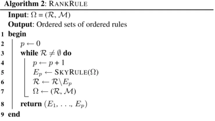
Algorithm 2: RANKRULE

Input:Ω = (R, M)

Output: Ordered sets of ordered rules begin 1 p← 0 2 whileR 6= ∅ do 3 p← p + 1 4 Ep← SKYRULE(Ω) 5 R ← R\Ep 6 Ω ← (R, M) 7 return(E1, . . ., Ep) 8 end 9

Example. In this example, we apply RANKRULEonΩ of Table 1. Since r1 and r4 are undominant rules then E1={r1, r4}. Now we

ignore r1and r4, the rules which are not dominated are r3and r6. In

fact, r3is dominated by only r1and r6is dominated by only r1, then

E2 ={r3, r6}. Now we ignore also r3 and r6, the rules which are

not dominated are r2 and r5. In fact, r2is dominated by r3 and r5

is dominated by only r6, then E3={r2, r5}. Finally, E4={r7, r8}.

This example is illustrated by Figure 4.1. The arrow indicates the process direction starting from the undominated rules. E1 contains

the top ranked rules which are them selves ranked within E1 from

left to right based on DegSim: r1is better ranked than r4.

4.2

Duality

RANKRULEperforms ranking by starting from the set of the most relevant rules (i.e., the undominated rules) and uses it to identify the next ranked set (i.e., the successor). Meanwhile, another dual perspective remains possible. It relies on starting from the set of the less relevant rules (i.e., rules that do not dominate other rules) and using them to identify the previous ranked rule set that we called predecessor set. We do not give a formalization of this dual

Figure 1. The output of RANKRULEapplied onΩ.

perspective, yet we explain how it works by the following illustrative example.

Example. We considerΩ of Table 1. First we identify the set of rules which do not dominate any other rules. These rules are r2, r7

and r8 then E4 ={r2, r7, r8}. Now ignore these rules. The rules

which do not dominate any other rules are r3and r5. In fact, r3

dom-inates only r2and r5dominates only r7and r8, then E1={r3, r5}.

Now we ignore also r3and r5, The rules which do not dominate any

other rules are r1and r6since they dominate r3and r5respectively,

then E2={r1, r6}. Finally, E1={r4}.

Figure 2. The dual RANKRULEapplied onΩ.

5

CONCLUSION

In this paper we proposed an approach that addresses the problem of rule selection and ranking. This approach is not hindered by the abun-dance of measures which is the issue of several works. These works have been devoted to measure selection in order to find one best mea-sure, whereas the real issue lies in selecting and ranking rules to help with decision making. We proposed two algorithms SKYRULEand RANKRULEto perform these two tasks based on the dominance re-lationship. When using our algorithms, the user does not have to

worry neither about the heterogeneity of measures nor about spec-ifying thresholds. As future works, we plan to formalize the dual of RANKRULEand to find the relationship between them that allows to obtain the output of one of them from the output of the other. Another importante prospective is to study the impact of any change within the relational tableΩ, such as the insertion of new measures of new rules, on the ranking or the selection.

REFERENCES

[1] R. Agrawal and R. Skirant, ‘Fast algorithms for mining association rules’, in Proceedings of the 20th Intl. Conference on Very Large

Databases, Santiago, Chile, pp. 478–499, (June 1994).

[2] J. Blanchard, F.Guillet, H.Briand, and R.Gras, ‘Assessing the interest-ingness of rules with a probabilistic measure of deviation from equi-librium.’, in The XIth International Symposium on Applied Stochastic

Models and Data Analysis, Brest, France, pp. 191–200, (2005). [3] S. Borzsony, D. Kossmann, and K. Stocker, ‘The skyline operator.’, in

ICDE, pp. 421–430, (2001).

[4] L. Geng and H.J Hamilton, ‘Choosing the right lens : Finding what is interesting in data mining’, in Quality Measures in Data Mining, ISBN

978-3-540-44911-9, pp. 3–24, (2007).

[5] M.J. Heravi and O. Zaiane, ‘A study on interestingness measures for associative classifiers., acm sac’10’, pp. 1039–1046, (2010).

[6] R. J. Hilderman and H. J. Hamilton, ‘Knowledge discovery and mea-sures of interest’, in volume 638 of The International Series in

Engi-neering and Computer Science, (2001).

[7] R. J. Hilderman and H. J. Hamilton, ‘Measuring the interestingness of discovered knowledge: A principled approach’, in Intelligent Data

Analysis 7, pp. 347–382, (2003).

[8] M. Klemettinen, H. Mannila, P. Ronkainen, H. Toivonen, and A. I. Verkamo, ‘Finding interesting rules from large sets of discovered as-sociation rules’, in Proceedings of the 3rd International Conference on

Information and Knowledge Management (CIKM’94),ACM Press, pp. 401–407, (November 1994).

[9] H.T. Kung, F. Luccio, and F.P. Preparata, ‘On finding the maxima of a set of vectors’, in J. ACM, vol. 22, no. 4, pp. 469–476, (1975). [10] F. Lenca, P. Meyer, P. Picouet, B. Vaillant, and S. Lallich, ‘Crit`eres

d’´evaluation des mesures de qualit en ECD’, in Revue des Nouvelles

Technologies de l’Information (Entreposage et Fouille de donnes), (1), pp. 123–134, (2003).

[11] P. Lenca, P. Meyer, B. Vaillant, and S. Lallich, ‘On selecting interest-ingness measures for association rules: User oriented description and multiple criteria decision aid’.

[12] M. Maddouri and J. Gammoudi, ‘On semantic properties of interes-tigness measures for extracting rules from data’, in ICANNGA (1),

Springer-Verlag, pp. 148–158, (2007).

[13] H. Manilla, ‘Methods and problems in data mining’, in Proceedings of

the 6th biennial Intl. Conference Database theory (ICDT’97), LNCS,V ol. 1186, Springer-Verlag, pp. 41–55, (January 1997).

[14] J. Matousek, ‘Computing dominances in En.’, in Inform. Process. Lett.,

38, pp. 227–278, (1991).

[15] M. Ohsaki, Y. Sato, S. Kitaguchi, and H. Yokoi, ‘Comparison between objective interestingness measures and real human interest in medi-cal data mining.’, in Orchard, R., Yang, C., Ali, M., eds.: 17th

inter-national conference on Innovations in Applied Artificial Intelligence (IEA/AIE 2004). Volume 3029 of Lecture Notes in Artificial Intelli-gence., Springer-Verlag, pp. 1072–1081, (2004).

[16] R.E. Steuer, ‘Multiple Criteria Optimization: Theory, Computation and

Application.’, in John Wiley, 546, (1986).

[17] P. Tan and V. Kumar, ‘Interestigness measures for association patterns: A perspective’, in Proceedings of Workshop on Postprocessing in

Ma-chine Learning and Data Mining, (2000).

[18] P. Tan, V. Kumar, and J. Srivastava, ‘Selecting the right interestingness measure for association patterns’, in Proceedings of the Eighth ACM

SIGKDD International Conference on Knowledge Discovery and Data Mining (ICDM’02), ACM Press, pp. 32–41, (2002).

[19] B. Vaillant, F. Lenca, and S. Lallich., ‘A clustering of interestingness measures.’, in Discovery Science. Volume 3245 of Lecture Notes in