HAL Id: insu-02537852
https://hal-insu.archives-ouvertes.fr/insu-02537852
Submitted on 10 Apr 2020HAL is a multi-disciplinary open access archive for the deposit and dissemination of sci-entific research documents, whether they are pub-lished or not. The documents may come from teaching and research institutions in France or abroad, or from public or private research centers.
L’archive ouverte pluridisciplinaire HAL, est destinée au dépôt et à la diffusion de documents scientifiques de niveau recherche, publiés ou non, émanant des établissements d’enseignement et de recherche français ou étrangers, des laboratoires publics ou privés.
non-Newtonian solution displacement
Nicole Mehr, Clément Roques, Yves Méheust, Skip Rochefort, John Selker
To cite this version:
Nicole Mehr, Clément Roques, Yves Méheust, Skip Rochefort, John Selker. Mixing and finger mor-phologies in miscible non-Newtonian solution displacement. Experiments in Fluids, Springer Verlag (Germany), 2020, 61 (4), pp.96. �10.1007/s00348-020-2932-x�. �insu-02537852�
Mixing and Finger Morphologies in Miscible
Non-Newtonian Solution Displacement
Authors: Nicole Mehr ([email protected]1), Clément Roques
([email protected])2, Yves Méheust ([email protected])3, Skip
Rochefort ([email protected])1, John S. Selker
Affiliations: 1Oregon State University, Biological and Ecological Engineering Department, OR, USA.
2ETH Zürich, Department of Earth Sciences, Sonneggstrasse 5, Zürich, Switzerland. 3University Rennes, CNRS, Géosciences Rennes, UMR 6118, 35000 Rennes, France
Corresponding Author: John Selker, [email protected] 541-737-6304
Abstract:
Unexpected interface complexities were found resulting from the miscible displacement of saltwater by a miscible shear-thinning solution (xanthan gum) in a radial Hele-Shaw cell, for both convergent and divergent flow. Such complex patterns have not been described before for either Newtonian or non-Newtonian solutions. A more viscous solution was injected into the cell to displace a less viscous solution (divergent flow) then withdrawn at the injection site
(convergent flow). A variegated mixing fringe between the solutions developed during the injection phase, against the stabilizing viscous effects, which would tend to promote a stable piston-like displacement. This interface geometry is markedly different from what is seen in displacement experiments performed with glycerol under otherwise similar viscosity contrast and flow conditions. The concentration field heterogeneity resulting from the presence of the fringe, quantified using a spatial autocorrelation measure, is mostly controlled by the applied shear rate, or equivalently, by the ratio of the volumetric flow rate to the flow cell’s aperture. It is
significantly correlated to the radial width of the mixing zone. In addition to producing a large volume of blended solution during the injection phase, the mixing fringe impacted the
development of viscous fingers (VFs) during the withdrawal phase. Such VFs are expected due to the viscosity ratio, but the initial roughness of the interface from which they develop, and, hence, their later dynamics, are controlled by the geometry of the mixing fringe at the end of the injection. We characterize the dynamics as a function of the imposed flow rate and cell
thickness. The observed complexities of miscible displacement involving shear-thinning solutions have implications for subsurface engineering applications such as oil recovery and groundwater remediation.
1. Introduction
Non-Newtonian fluids, which are found in a wide range of industrial and environmental applications, have a viscosity which is dependent on flow conditions. In geological applications, non-Newtonian fluids are used to facilitate delivery of remediation materials into the subsurface by providing access to lower permeability regions, which are frequently missed by traditional methods (Martel et al., 2004; Zhong et al., 2013). Particularly, shear-thinning fluids, whose viscosity decreases with shear rate, are commonly used to suspend particles in material for subsurface remediation to improve solute transport (Zhong et al., 2013). Non-Newtonian fluids are used during oil recovery in a secondary process to displace oil in porous reservoirs (Gleasure & Phillips, 1990) and are also used as additives to food products and pharmaceuticals to provide stability and suspension (CPKelco, 2008). The wide variety of applications for Non-Newtonian fluids displacing Newtonian fluids highlights the importance of investigating this unique type of fluid interaction.
Non-Newtonian fluids are primarily characterized into two subgroups: shear-thinning fluids (viscosity decreases with increasing shear) and shear-thickening fluids (e.g., Mezger, 2014). The dynamic viscosity of non-Newtonian fluids produces complex flow patterns in porous and fractured media. For monophasic flows, while their hydraulic behavior is far from fully understood, it is generally observed that shear-thinning fluids result in more heterogenous or “preferential” flow paths. The monophasic flow of shear-thickening fluids is less understood, but includes complexities such as jamming (Brown & Jaeger, 2014; Fall et al., 2008)
In dual-viscosity displacement processes, the interface between two fluids is viscously-unstable when the lower viscosity fluid invades, regardless if the fluid is Newtonian or non-Newtonian (e.g., Saffman and Taylor (1958); Linder et al., (2002)). If no other mechanism, such as a density contrast between the two fluids, balances the viscous instability, instabilities
percolate in viscous fingers (VF) of flow through the defending fluid, much of which will remain behind the advancing front (Lindner et al., 2002). Note that a non-zero density contrast between the fluids will result in a buoyancy effect on the interface, which will be either stabilizing (if the denser fluid is below) or destabilizing (otherwise). In the former case, gravity can stabilize an otherwise viscously-unstable interface (see Méheust et al. (2002), Lovoll et al. (2003)).
VF are commonly observed in subsurface engineering applications, including oil
recovery (Gorell & Homsy, 1983), and yet their impact on the spatial distribution of fluid phases and solute concentrations, inside the permeable medium, is still not fully understood for many types of fluids and geometries. These unstable interfaces can be costly, for example by
diminishing oil recovery (Gorell & Homsy, 1983) or resulting in poor mixing of fluids injected to promote groundwater remediation (Tosco & Sethi, 2010).
VF arising from unstable interfaces have been studied using Hele-Shaw cells (among other setups, see i.e. Toussaint et al., 2012), which are flow cells consisting of horizontal closely-spaced parallel transparent plates to simulate two-dimensional Darcy flow (Hele-Shaw, 1898). The Hele-Shaw geometry is in particular relevant to investigate fluid displacement in fractures, if one neglects the roughness of the fracture walls. Hele-Shaw cells have typically been constructed using a linear or radial injection geometry and experiments have used both immiscible and miscible fluids.
Immiscible fluid displacement, where surface tension between the two fluids results in so-called capillary forces acting at the fluid-fluid interface, has been studied for Newtonian fluids in both linear (Bonn et al., 1995; Chevalier et al., 2006; Miranda & Widom, 1998; Saffman &
Taylor, 1958) and radial (J. Den Chen, 1989; Dias et al., 2012; Miranda & Widom, 1998; Thomé et al., 1989; White & Ward, 2014; Yang et al., 2019) Hele-Shaw cells. Miscible Newtonian fluids, where mixing between the injected and displaced fluids takes place during the
displacement, gives rise to more irregular fingering patterns than what is observed for immiscible fluids (J. Den Chen, 1989). Miscible fluid displacement has also been studied in both linear (Boschan et al., 2003; Malhotra et al., 2015; Mishra et al., 2010) and radial (Bunton et al., 2017; C. Y. Chen et al., 2010; J. Den Chen, 1989; Chui et al., 2015; Daccord & Nittmann, 1986; Paterson, 1985; Pons et al., 1999) Hele-Shaw cells.
For miscible fluids, linear geometries represent a simple case, where effects of changing curvature of the interface are negligible. In contrast, for radial geometries, curvature gives rise to complex effects such as fingertip splitting (Miranda & Widom, 1998). Although there is an abundance of literature on VF in Newtonian fluids in both geometries, the more complex VF involving non-Newtonian fluid(s) has not been thoroughly studied.
Previous experimental and theoretical studies have observed considerable differences between instability development for Newtonian and non-Newtonian fluids. For instance, studies have found that tip-splitting, a common observation in Newtonian fluids, is suppressed in shear thinning fluids in radial Hele-Shaw cells (Amar & Poiré, 1999; Fast et al., 2001). Lindner et al. (2002), observed that rigid, strong shear-thinning fluids have smaller finger widths than a comparable Newtonian fluid in a linear Hele-Shaw cell. Lindner et al (2002) explained that relatively small finger widths have been observed in Newtonian fluids when anisotropy is present i.e., a bubble on the interface as described by (Couder et al., 1986). The small finger widths in shear-thinning fluids arise from anisotropy at the tip of a finger where shear is greater (thus viscosity is lower) than on the finger sides (Lindner et al., 2002). Lindner et al. (2002) also observed that finger width decreased as the gap between the two linear cells increased. On the other hand, Daccord & Nittmann (1986) found that the finger width of miscible shear-thinning fluids increased as the gap between the two radial cells increased.
Other notable studies have looked at both non-Newtonian miscible and immiscible displacement in linear cells, which significantly constrains the direction of fluid flow (Bonn et al., 1995; Boschan et al., 2003; Sader et al., 1994). Only a few have studied radial miscible displacement (Lemaire et al., 1991; Obernauer et al., 2000) while more have studied radial immiscible displacement (Amar & Poiré, 1999; Fast et al., 2001; Lemaire et al., 1991; Sader et al., 1994; White & Ward, 2014). Lemaire et al. (1991) used highly viscoelastic fluids to map visco-fracturing patterns. Obernauer et al. (1994) studied the transition phase from stable to unstable displacement for divergent flow. Obernauer et al. (1991) concluded that the transition phase was a result of the nonlinear viscosity variations along the fluid interface. The full phenomenology of VF in a radial Hele-Shaw cell with miscible, shear-thinning fluids, remains an open question.
We use a radial Hele-Shaw cell to avoid any potential effect of lateral boundaries on the flow behavior. The radial configuration is also more consistent with what occurs in the field with injection and withdrawal from a borehole. However, radial geometries give rise to more complex fingering patterns and involve an additional complexity, which renders their study more difficult: in a radial injection geometry, the mean flow velocity at a given distance from the injection site decreases as a function of distance and thus so does the magnitude of the viscous forces.
Previous research using non-Newtonian fluids in a radial Hele-Shaw cell typically focused on divergent flow as a less viscous fluid is injected into the cell to displace a more viscous fluid. To the best of our knowledge, no previous study has researched both convergent
and divergent flow for miscible non-Newtonian solutions in a radial Hele-Shaw cell, by injecting a more viscous non-Newtonian solution (xanthan gum in this study) into the cell to displace a less viscous resident Newtonian solution (saltwater in this study) and withdraw both solutions back into the injection site. In this setup, the divergent flow regime is stable with no VF present while the convergent flow regime is unstable with VF present. By both injecting and
withdrawing, we perform an analog simulation of what would occur in the field during subsurface engineering applications involving injection of a shear-thinning solution with divergent flow followed by convergent flow, a configuration denoted as “push-pull” in subsurface engineering.
This research aims to characterize miscible radial instability morphology and dynamics for the injected shear-thinning solution, xanthan gum, and the resident saline solution in both divergent and convergent flow configurations. We specifically seek to quantify how changes in aperture and flow rate impact the displacement of the saltwater by the non-Newtonian solution in a radial Hele-Shaw cell and to describe the morphological properties of the instability arising from miscible radial flow conditions. This study contributes to a better understanding of the physical processes at play when a shear-thinning solution both displaces and is displaced by water in the subsurface, as would be the case in a number of extraction, remediation, and characterization procedures.
2. Methods
2.1 Characterization of Solutions
A xanthan gum (XG) unit is composed of two glucose, two mannose, and one glucuronic acid and has an approximate molecular weight of two million Daltons, but the molecular weight depends on the size of the XG aggregates (molecular entanglements). The units of XG form a double helix. When shear is applied, the aggregate of XG begins to unfold and the molecules disentangle and align (CPKelco, 2008). The XG helix will also unfold if XG is not mixed in an ionic salt solution, which will impact the rheological properties of the solution (Lecourtier et al., 1986). Suspending XG in a salt solution allows the XG molecules to be homogeneously folded and minimizes the thixotropy effects, i.e., the viscosity of the XG does not vary in time at a constant shearing rate and thus its shear-thinning properties only depend on the current shear rate rather than the complete shear rate history. We can then consider that a given concentration of XG under a specific rate of shear will have a reproducible viscosity.
We have selected the most clarified, highly-filtered, highest food-grade XG from the KELTROL line at CP Kelco, xanthan gum T622 (material number 20000625), for this study and have selected the minimal salt concentration for the solution (1.5%) to prevent conformational changes, i.e., ensuring that the double helix remain folded.
XG was hydrated with deionized water and was homogenized using a high shear mixer to prevent microgel formation. Microgels are submicron polymer colloids which form if the
solution is not hydrated properly and can significantly alter the rheology of the solution and impact the flow in the Hele-Shaw cell (Abdulbaki et al., 2014). A simple 0.45-micron membrane filtration analysis was applied to make sure that there were no microgels remaining in the XG solution.
XG solution of concentration 0.3 wt.% xanthan gum, 1.5 wt.% sodium chloride, and 0.025 wt.% food grade dye was used as the injected solution. The dye was added to optically
distinguish the injected solution from the resident solution in the Hele-Shaw cell. At the
specified concentration, the addition of powdered dye to the XG solution was shown to have no effect on the solution’s rheological properties (Online Resource 1.A).
The 0.3 wt. % concentration of XG exhibits strong shear-thinning properties. It is above the critical concentration (C*) to ensure polymer-polymer interactions and is therefore weakly viscoelastic. At high concentrations, XG has a low degree of thixotropy and therefore would show no thixotropic effects at the low chosen concentration and with the addition of 1.5% salt. The rheology of the solution was measured with oscillatory and flow sweeps using a stainless-steel, cone and plate geometry on a DHR-3 rheometer prior to each experimental run to ensure the reproducibility of the XG solutions’ rheology. The rheological data was obtained at a
temperature of 25°C. The shear rates tested using the rheometer were typically from 0.01 to 100 1/s (Online Resource 1.B). However, a few solutions were tested with shear rates down to 0.001 1/s to make sure the rheological properties were consistent at lower shear rates. . Our XG
solution behaves as a power-law fluid over the range of shear rates tested. A power law rheology was found to fit the XG viscosity and shear rate curves with a power law index of n=0.3 (0<n<1) and a consistency index of k=1.0 Pa.s2, that is (Online Resource 1.B,1.C)
𝜂 = 𝑘𝛾̇& Eq. 1
with 𝜂 being the viscosity, k being the flow consistency index, 𝛾̇ being the shear rate and n being the power law index.
Note that this rheology is relevant to our experiments, since the shear rates observed in the experiments fall in the range investigated by the rheology measurements. Indeed, the largest flow velocity was encountered with the largest investigated flow rate (20 ml/min), at the outlet of the injection tube (at a distance from the cell center ~ 3 mm), and in the thinnest Hele-Shaw cell (of thickness 0.72 mm); this largest flow velocity thus amounted to ~ 17 mm/s. Dividing it by the half-thickness of the cell, we obtain a rough estimate of the largest shear rates encountered in the flow cell during our experiments: ~ 80 s-1. Similarly, the smallest velocity encountered in the experiments occurred at the cell’s perimeter (of radius ~ 15 cm), in the cell of largest thickness (2.5 mm) and for the smallest volumetric flow rate used: 0.25 ml/min; that smallest velocity is therefore close to 0.2 mm/s, and by dividing it by the largest cell’s half-thickness (1.25 mm) we can estimate the smallest shear rate encountered in the flow cell throughout all experiments to 0.2 s-1 .
C* was determined by measuring the viscosity as a function of the shear rate at concentrations ranging from 0.01% to 1wt% XG (Swann, 2017), plotting the zero-shear viscosity vs concentration, and determining the point where the slope of that plot deviates from linear upwards, thus indicating that molecular interactions have occurred. C* was determined to 0.026 wt%. Our XG concentration is above C*, therefore the yield stress is negligible (Online Resource 1.D). The size of the region close to the Hele-Shaw cell’s mid-plane, where the shear stress potentially may be less than the weak yield stress, is vanishingly small and therefore the yield stress of XG can be considered negligible in the entire volume of the cell.
2.2 Experimental Setup
A radial Hele-Shaw cell consisting of two horizontal parallel glass plates with diameters of 305 mm, separated by a specified distance with micrometers, was used in a temperature-controlled dark room (Figure 1). The temperature of the room was kept at a constant 18°C.
Fluorescent lamps were installed underneath the Hele-Shaw cell. A transparent greyscale reference card was placed on the top glass plate to monitor light fluctuations. The experiment was carried out in a black windowless room with additional black-out curtains, which surrounded the experimental setup to prevent optical interference. A Canon EOS 50D camera with an EF-S 18-200 mm lens was situated 127 cm above the Hele-Shaw cell and set to take a Canon RAW image once every second. RAW images were used to obtain the highest level of image
information prior to processing. The resolution of the images was 15 pixels per millimeter (TIFF format).
To prepare for the injection phase by purging the system of any resident solution, with the top glass plate removed, a purge-tube was inserted into the top of the bottom glass plate at the injection site (to prevent contamination of the cell). A syringe was filled with XG solution and was kept free of any gas bubbles. The syringe was secured to the pump and was attached to the tubing connected to the center of the Shaw cell. XG solution was pushed into the Hele-Shaw cell until it purged through the temporary purge tube. Then approximately 250 ml of 1.5 wt. % saltwater was poured onto the bottom glass plate. The purge-tube was removed and the top glass plate was placed on so that the gap between the plates was entirely filled with the saltwater solution. The syringe pump was programmed to inject the specified volume of solution at the specified injection rate. After the solution was injected, the direction of the syringe pump was reversed with the same volumetric flow rate, which initiated the withdrawal phase. The diameter of the injection/withdrawal site was approximately 3 millimeters.
The flow rate was held constant for both the injection and withdrawal phases and varied between experiments from 0.25 mL/min to 20 mL/min. A uniform aperture (gap) was imposed between the two glass plates using micrometers (with a precision down to a thousandth of a mm and validated using feeler gauges) and ranged between 0.254 mm and 2.54 mm. The injection volume was either 5 mL for small apertures or 10 mL for larger apertures.
2.3 Image Analysis
Images were processed using methods by (Sumner, 2014) and a concentration calibration curve figure can be found in Online Resource 1.E. The concentration calibration curve was constructed using the Beer-Lambert Law, additional details and equations can also be found in the Online Resource 1.E (including a figure of the calibration curve). VF were determined by converting Cartesian coordinates (X, Y) of the solution interface to radial-curvilinear coordinates (r, S). r corresponds to the radial distance to the injection site and S corresponds to the position along the perimeter of the interface (Chui et al., 2015). The r values were inverted and maxima were identified using a prominence value as a threshold. The positions of the maxima were converted to Cartesian coordinates and mapped back onto the interface and were tracked in time. The maxima’s identified are representative of the tip of the VF. Minima’s were also identified in the code, which represent the upper boundaries of the VF. Polygons were constructed using the maxima’s and minima’s to determine the polygonal area of the VF. The length of the VF was determined by the distance between the maxima (tip of the VF) and the midpoint of the line segment connecting the two minima on either side of the maxima. Width of the VF was determined by dividing the polygonal area of the VF by the length of the VF.
In this section, the results are presented as a detailed analysis for both the injection (stable displacement) and the withdrawal (unstable displacement) phases. Observation of the injection phase validates the relationship between pumping rate, total injection and aperture employed in the experimental setup. We also discuss unexpected observations regarding the development of a mixing fringe during the injection. The morphology and dynamics of VF, which arise during the unstable displacement during the withdrawal phase, are described. The variability in finger morphology and withdrawal interface evolution dynamics is quantified and discussed. The phenomena described in the results section were observed in all 16 experiments, which had various apertures and flow rates. Experiments were repeated many times in the development of the experimental protocol (data not shown), yielding qualitatively consistent behaviors for similar apertures and fluxes. The following results discussed in figures were selected to show representative examples.
3.1 Injection Phase (Stable Displacement)
During the injection phase, the viscosity of the displaced solution (saltwater) is always smaller than that of the displacing solution (XG solution), so that no viscous instability of the interface is expected (i.e., no VF). For miscible displacement of a Newtonian solution by a Newtonian solution, the concentration field of the mixing species would be expected to only have a radial dependence. Any behavior different from this must be attributed to the rheological properties of the polymer. To ensure that our observations could be attributed to the properties of a non-Newtonian behavior of XG, a series of experiments (whose data is not shown here) were run using the Newtonian fluid, glycerol. A mixing fringe (to be discussed later) was not observed during the injection phase of the glycerol experiments.
The interface velocity of the injected XG was tracked with radial distance, r. Introducing the flow rate Q, the volume of solution injected during duration dt is Qdt and thus, due to the solutions’ incompressibility is also equal to 2pra dr, where a is the flow cell’s aperture. The
average interface velocity, dr/dt, is thus expected to follow a 1/r relationship (Eq. 2), which is indeed confirmed by the data (Online Resource 1.F).
𝑑𝑟 𝑑𝑡 =
𝑄 𝑎 ∗ 2𝜋𝑟
Eq. 2
Three prominent regions of solution were observed in the injection phase (Figure 2): a region of essentially pure displacing (invading) solution; a region of pure displaced (resident) solution; and a mixing zone. A mixing zone was observed in all experiments, consistent with the dispersion associated with the parabolic velocity profile across the vertical section of the Hele-Shaw cell. However, rather than the concentration profiles one would expect from the interaction between advection by creeping flow and molecular diffusion, which would be smoothly-varying and only in the radial direction, a variegated mixing fringe was observed for experiments with apertures equal to or less than 0.762 mm and flow rates higher than 3 mL/min. The mixing fringe creates an irregular interface (Figure 2C) when compared to the smooth orthoradial interface seen in larger aperture/lower flow experiments (Figure 2A). In other words, the XG
concentration does not only depend on the radial coordinate.
The mixing zone region was defined as the ensemble of all locations at which concentrations fall in the range between 70 and 90% of that of the influent XG solution. To
determine the mixing zone’s dynamics with respect to time, the width of the mixing zone was plotted against the total volume of injected solution (Figure 3). Four representative experiments with and without a mixing fringe were plotted (one set with a fast injection/withdrawal rate and another set with a slow injection/withdrawal rate). The superscript numbers in the legend of the figure correspond to the experiment number, which is discussed later on. Despite these four selected experiments exhibiting mixing zones that look entirely different from each other, the mixing zone width was found to grow at a similar rate for all experiments regardless if a mixing fringe was present. Generally, the normalized mixing zone width remained constant while the volume of solution injected increased. However, the 0.762 mm aperture experiments had a mixing fringe present and those showed a slight decrease in the normalized mixing zone width with respect to volume. Note that in the absence of a mixing fringe, the growth of the mixing zone should result mostly from a process similar to the Taylor-Aris diffusion, i.e., the interaction between molecular diffusion and advection by a velocity field that is heterogenous across the thickness of the Hele-Shaw cell. The difference between the Taylor-Aris diffusion per se is that the latter involves a parallel flow and a fixed volume injection of solute rather than a continuous injection. Hence, the widening in time of the mixing zone is expected to be a diffusive process. Here it seems that the process is not impacted as much by the presence of a mixing fringe.
To quantitatively determine the presence of a mixing fringe (i.e. whether the mixing zone features a mixing fringe or not), local Moran’s I spatial autocorrelation methods were used. Spatial autocorrelation measures how similar or dissimilar values (concentrations) are to one another with respect to their spatial location. Local Moran’s I methods determine the degree of spatial autocorrelation within each sub-unit in a matrix by using local indicators of spatial association and a moving window (Fu et al., 2014). The local Moran’s I values were calculated using a Matlab function on Matlab’s File Exchange (Hebeler, 2016). The function calculated local Moran’s I for a grid using a weight matrix. In our case, the grid is a normalized
concentration matrix of the mixing zone only. The start of the withdrawal phase image was used in this analysis for all experiments. The function computed a matrix of the local Moran’s I values. The sum of the squares of the local Moran’s I were used as a metric to quantify the small-scale fluctuations of the concentration field, which are indicative of whether there is a mixing fringe or not.
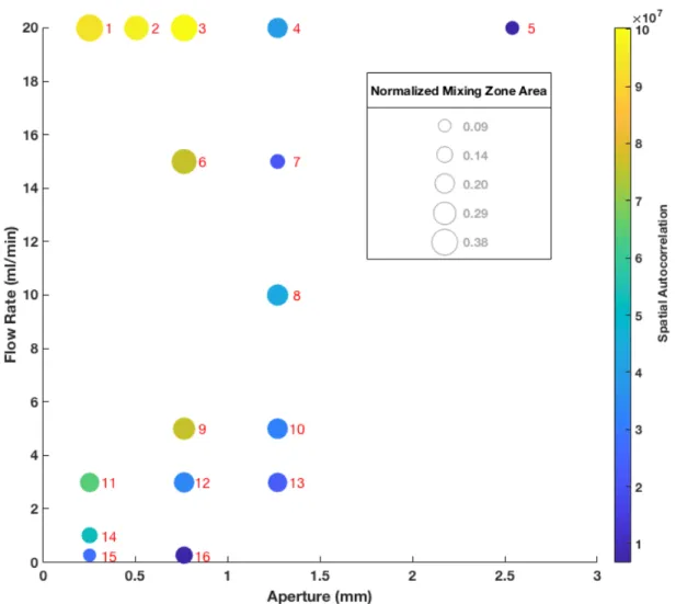
A phase diagram was created for all investigated apertures and flow rates (using the last image of the injection phase) where the spatial autocorrelation results are plotted as the color of the data point for the mixing zone regions (Figure 4), in order to infer how the existence of a mixing fringe depends on aperture and flow rate. Each experiment plotted in the phase diagram has a corresponding number, which will be referenced in other figures. The size of the data points represents the proportion of the invaded area that is occupied by the mixing zone. The mixing zone region was defined as the ensemble of all locations at which concentrations fall in the range between 70 and 90% of that of the influent XG solution. Data points of high spatial autocorrelation (i.e., areas where local XG concentration varies over short spatial scales) indicate the presence of a marked mixing fringe, while areas of low spatial autocorrelation indicate regions of a less marked mixing fringe or the absence of the mixing fringe (mixing zone only). At a constant injection rate, the size of the mixing fringe increased as aperture decreased. At a constant aperture, the size of the mixing fringe increased with flow rate. This relationship is qualitatively shown in the concentration images in Figure 5.
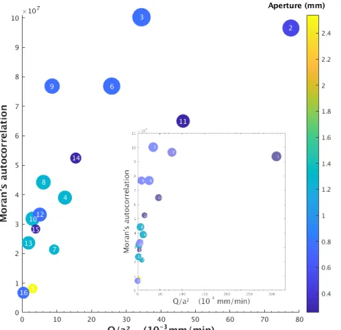
In fact, since the mixing fringe is related to the shear-thinning rheology of the solution (since it is not seen when displacing the saltwater with glycerol), the main control parameter
must be Q/a2. To check this dependence, we have plotted the Moran’s I autocorrelation as a function of Q/a2 in Figure 6. The Moran’s I autocorrelation is much more correlated to Q/a2 than it is to either Q or a separately, as seen in the phase diagram. This is confirmation that the existence of a mixing fringe and how marked the mixing fringe is are both shear-dependent.
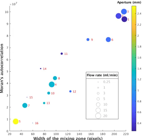
In addition, the presence of a mixing fringe, as inferred from the Moran’s I
autocorrelation, happens to be significantly correlated to the width of the mixing zone, as shown in Figure 7. The correlation between the two variables is quite striking.
3.2 Withdrawal Phase (Unstable Displacement)
3.2.1 Morphological Characterization of the Withdrawal Phase
In the withdrawal phase, the interface is expected to be viscously unstable since the displacing solution (saltwater) has a lower viscosity than the XG. An onset time for the
instability was observed as the withdrawal phase began, i.e. the time it took VF development to become apparent along the perimeter of the interface. Prior to the onset time, the regions of XG and water retreated toward the injection site while preserving a semi-radial interface before instability development became apparent. A dilute residual film of XG on the glass plates was observed. The film remained stationary as the rest of the solution moved towards the injection site (Figure 2B).
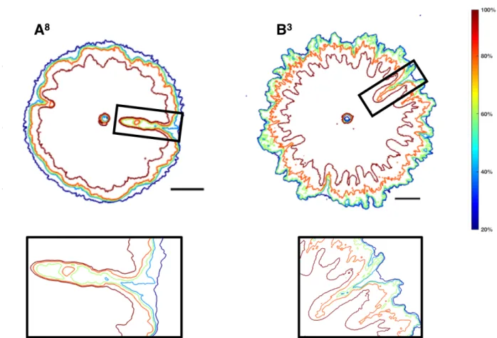
Stationary regions of XG were isolated as VF began to develop along the once stable interface (Figure 2B). The resident water invaded the XG and formed fingers, which were regions of lower XG concentration and water penetrating into the injected concentration of XG and were a function of the concentration gradient (Figure 8). Figure 8 shows two contour maps representative of what was observed in all the experiments with and without a mixing fringe. In experiments that had a mixing fringe present in the injection phase, contour lines of the
concentration field show concentric lines, which indicate a superposition of a moderate radial gradient in concentration to the VF geometry, resulting in three regions: one occupied by the pure water phase, one occupied by the XG phase, and between them a region of diluted mixing fringe phase. Note that in the following text, this geometry is sometimes referred to as
“concentric fingering.” The invading water was observed to penetrate through the center of the VF, made up of solution drawn from the mixing fringe, where concentrations of XG were low and created a poorly-defined inner-boundary, while the surrounding regions of higher XG concentrations outlined a second finger boundary (Figure 8). The outer-finger boundary, formed in the high-concentration regions of the VF, took on a smooth and well-defined finger shape, resembling that of a Saffman-Taylor finger (Saffman & Taylor, 1958). In contrast, the invading water finger inner-boundary, formed in the low concentration regions of the VF, took on an irregular variegated shape.
When the first finger reached the injection site (breakthrough), it formed a preferential water pathway where a stream made up primarily of water exited the Hele-Shaw cell through the injection site. A well-defined water channel then formed, and occasionally sheared off patches of the stationary regions of XG which would often move as blobs or islands surrounded by faster moving water. In addition to XG movement toward the injection site, XG was also sheared off by the moving water in multiple directions from the outer perimeter of the stationary XG regions and pushed through the existing water channel.
The VF geometry described above has not been documented for non-Newtonian solutions. Figure 9 highlights the differences in finger formation for a Newtonian and a
non-Newtonian solution, all experimental parameters being otherwise identical. The non-Newtonian fluid, glycerol, promoted the formation of VF almost everywhere along the solution interface. The non-Newtonian solution, XG, promoted the formation of a select few VF along the interface with most of the solution being stationary, which can be attributed to its shear-thinning nature (Figure 9). The shear-thinning nature allows for more pronounced flow localization of the shear-thinning solution when compared to creeping flow in a Newtonian solution (Lindner et al., 2002).
3.2.2 Morphological Quantification of the Withdrawal Phase
Perimeter of the XG interface and area of the XG region were determined for both the injection and withdrawal phases (Figure 10). Both the perimeter and area were calculated using Matlab’s built-in Regionprops function, which measures various properties of image regions. There was a time lag between the start of the injection phase and end of the withdrawal phase due to hysteresis of the syringe pump. Pressure data was collected to confirm that all solution was stationary during this lag time, until the syringe pump hysteresis ended (Online Resource 1.G). The pressure data was obtained using an inline pressure sensor that was developed for this project. A MS5803-02BA pressure sensor with operating temperatures from 30 kPa to 110 kPa, with accuracy of plus or minus 0.15 kPa, and precision of 0.00024 kPa was used. The sensor was fitted into a 3D printed adaptor to fit the experimental tubing (Measurement, 2017). After the withdrawal phase began, the solution interface decreased in perimeter as the regions of XG and water retreated toward the injection site while preserving the stable interface. The solution interface then started increasing in perimeter when the instabilities formed.
The onset of apparent instability development is observed in a plot of perimeter vs. volume of XG in the cell (Figure 11). For experiments with the same aperture, but different flow rate, instability formation occurred earlier for the lower flow rate. For experiments with the same flow rate, but different aperture, instability development occurred earlier for the lower aperture. The volume of XG which remained in the cell after breakthrough of the first finger is also a function of flow rate (Online Resource 1.H). This suggests that higher flow rates created a
relatively low viscosity ratio between the XG and the water since the XG experienced high shear. The viscosity ratio drives instability development. Therefore, the low viscosity ratio between the XG and the water delayed the formation of VF development along the interface during the withdrawal phase. The delay in finger formation allowed the interface to remain stable for longer, thus allowing more of the XG to exit the cell. The opposite holds true for low flow rates. Instability development occurred earlier for experiments with smaller apertures (with the same flow rate) because the smaller apertures allowed for a higher shear rate, which promoted the formation of the mixing fringe during the injection phase. In addition, the mixing fringe created more defects along the interface, thus allowing more locations of instability development to take shape and form earlier during the withdrawal phase.
To determine the impact of the mixing fringe on the withdrawal process, experiments with a slow injection rate of 1 mL/min and faster withdrawal rate were completed for an aperture of 0.762 mm. The slow injection rate was used to minimize the formation of the mixing fringe during the injection phase. The volume of XG left in the cell for experiments with a slow injection rate and fast withdrawal rate are also plotted in Online Resource 1.H. The slow
injection rate experiments (no mixing fringe) were found to have less XG volume left in the cell than their comparable fast injection rate experiments (mixing fringe). Thus, the push-pull experiments performed with a slow injection rate (no mixing fringe) began forming fingers at later times than the fast injection rate experiments (mixing fringe). In contrast, the fast injection
rate (mixing fringe) experiments formed fingers at earlier times. This can be attributed to the fact that when a mixing fringe is present at the beginning of the withdrawal phase, the initial
perturbation that results in finger growth is already finite and in some cases, quite developed. The mean radial distance of the interface was plotted as a function of time for the withdrawal phase. At early times, a good agreement with the predicted mean radial distance, assuming a simple mass conservation relationship, was found. From Eq. 2 above, integrated between time 0 at the start of the withdrawal phase (at which the radial distance is R0) and time t (at which the radial distance is r), one obtains
Eq.3
𝑟/01234512 = 6(𝑅9: −
𝑄𝑡 2𝜋𝑎)
where Q is the volumetric flow rate. As expected, the prediction works well for early times, before instabilities form (Online Resource 1.I). After instabilities form, the experimental mean radial distance becomes smaller than the predicted value for a stable withdrawal. Once the first finger reached the injection site, the system reached a quasi-steady state.
The number of fingers formed during each withdrawal experiment is shown in Figure 12 as a function of flow rate and aperture. Since, except for very small apertures, the number of fingers seems to depend more on the aperture than on the flow rate, we have performed an exponential fit of experimental number of fingers vs. aperture for all experiments (see inset in Figure 12) and show the fit values as colored squares around the disk-shaped data markers. As expected, this “prediction” works decently well (R2=0.82) except for the smallest apertures. It is observed that the actual number of fingers formed in a given experiment, is strongly dependent on the aperture.
The “concentric fingering” complicates the determination of a representative
characteristic finger width. To quantify individual finger widths, concentration thresholds were used to visualize the finger geometries at 50% and 90% XG concentrations. For a given
experiment, only the final time (interface/image) before the first finger reached the injection site was used since the fingers are well developed at this time. The 90% threshold finger widths represent the outer boundary of the VF and were found to have a larger width than the 50% threshold finger widths, which represent the inner boundary of the VF (Figure 13). Finger length was also determined and compared to width for 50% and 90% thresholds (Figure 14). The results show that there is no well-defined or representative finger width for a given experiment with respect to aperture, which makes comparisons to previous studies difficult. Finger width development with respect to time was investigated, but no pattern or relationship was found, which would be expected for a Newtonian solution (results not shown here). The observed morphology of VF during miscible displacement is considerably more complex and dynamic in the flow configuration addressed in this study than what has previously been described in the literature (Daccord & Nittmann, 1986; Obernauer et al., 2000).
4. Discussion
Although some dynamics and morphologies described above have not previously been explored, certain morphologies of fingers observed during our experiments are similar to those already described in the literature. As VF developed along the interface, one finger grew faster than others and reached the injection site first. This is known as finger competition, and has been documented before for Newtonian fluids (Miranda & Widom, 1998; Saffman & Taylor, 1958; Thomé et al., 1989). The residual film of the displaced solution (XG) on the glass plates has also been documented and studied for both Newtonian and non-Newtonian fluids (Lindner et al., 2002; Saffman & Taylor, 1958; White & Ward, 2014). The film did not interfere with image analysis techniques because its low concentration was not included in concentration thresholds and was therefore negligible in our current experiments. Future work should include
quantification of the film thickness on the glass plates to compare to Newtonian findings to determine if there are differences in the volume of film left behind. Our experimental data prior to the development of an instability followed the theoretical predictions for velocity and mean radial distance in both the injection and withdrawal phases, which is consistent with a
convergent/divergent flow at a constant imposed volumetric flow rate. Comparison of the results obtained in these experiments using XG to those obtained in experiments where the injected solution was glycerol, in the same Hele-Shaw cell, further show that our results are directly related to the shear-thinning nature of the XG.
4.2 Unexpected Patterns of the Injection & Withdrawal Phases
The mixing fringe formed during the stable injection phase for which the interface is viscously-stable, was unexpected and to the best of our knowledge, has not been previously observed in Newtonian or non-Newtonian fluids. Several factors could have influenced the formation of the mixing fringe: turbulence, diffusion, elongation and molecular structure. The mixing fringe forms at low creeping Reynolds numbers (Re<<1), therefore the mixing fringe does not result from non-linearities in the flow. The relaxation time of the XG is lower than the flow rates used, therefore elastic effects are not significant at the mixing fringe. The relaxation time of the XG solution was determined using a dynamic oscillatory shear experiment to measure the dynamic storage (G’) and loss moduli (G’’) as a function of frequency. The inverse of the crossover frequency (where G’= G’’), is often used to determine the maximum polymer relaxation time. The Weisenberg number (We#), defined as the shear rate x polymer relaxation time, is a measure of the expected importance of elastic effects in a flow field. We# > 1.0 is the point where elastic effects can be expected to become important. In the mixing fringe, the Weisenberg number is smaller than 1, so elastic effects are not expected to be significant. In addition, there is no measurable elastic normal stress in steady shear experiments at the shear rates observed in the mixing fringe. The molecular weight of XG has been reported in the range of 2-50 million Daltons (CPKelco, 2008; Dintzis et al., 1970). The hydrodynamic length of 600-2000 nm with a hydrodynamic diameter of 2 nm for XG are much smaller than the apertures used in our
experiments (Rodd et al., 2000). Note that the size of the XG molecules is listed as a range because the size and weight depends on the amount of molecular entanglements (CPKelco, 2008). This suggests that the mixing fringe is not related to an interaction between
hydrodynamics and the microstructure of the XG, but is a purely hydrodynamical phenomenon. In non-Newtonian fluids, dendritic and tip-splitting patterns arise from the characteristic anisotropic properties of the microstructure, specifically the shear rate dependence of viscosity (Fast et al., 2001). Given that the mixing fringe is a function of aperture and flow rate (Figure 4), the mixing fringe could be a result of the anisotropy of the XG. This is consistent with our
observation that the fringe formation is shear dependent (Figure 6), as the largest mixing fringe was observed in the highest injection rate and smallest aperture. At high shear rates, the XG solution experiences a large decrease in viscosity, leading to the XG’s diffusion coefficient to increase to a large extent in the solution, and thus hypothetically allowing it to disperse faster into the resident water. This may suggest that there is a shear threshold for the presence of the mixing fringe and should be investigated further. We note that the diffusion coefficient associated with such massive molecules, computed with the Einstein-Nernst equation, as expected, is very low and was found to be on the order of 10-17- 10-16 m2/s (Online Resource 2). Therefore, we conclude that diffusion does not play a significant role in the development of the mixing fringe.
To the best of our knowledge, such a mixing fringe has not previously been documented for non-Newtonian fluids. Fast et al. (2001) conducted a similar experiment with an immiscible non-Newtonian fluid in a radial Hele-Shaw cell and concluded that under certain cases elastic effects can be neglected, allowing shear-thinning fluid flow to simplify to that described by the generalized Darcy equation used for Newtonian fluids. The XG concentration used in our experiments is above the critical concentration (C*) to ensure polymer-polymer interactions and is therefore weakly viscoelastic. Our experimental results may complicate Fast et al.’s (Fast et al., 2001) simplification for miscible fluids, as the presence of the mixing fringe may inhibit the ability to simplify fluid flow for miscible cases.
The mixing fringe experiments show a slowly varying XG concentration on the boundary of the VFs, which is not observed in experiments with no mixing fringe present. This makes the prediction of a unique finger width and velocity difficult, which has been a primary way of characterizing instability development in the literature (data on VF velocity not shown). Therefore, a range of concentration and viscosity gradients needs to be analyzed when quantitatively characterizing instability development. Daccord & Nittmann (1986), studied a miscible non-Newtonian fluid with a shear-thinning exponent of n=0.15 and found the finger width to be linearly-dependent on the flow cell’s aperture, for apertures between 0.1 to 1.2 mm. Our experiments used aperture ranges from 0.254 to 2.54 mm and our results in (Figure 13 & 14) show that we do not observe such a trend since there is no well-defined finger width for a given aperture for either the 50% and the 90% thresholds. Therefore, it must be investigated as to why our miscible non-Newtonian solution has produced results at odds with those of Daccord & Nittmann (1986).
5. Conclusion
We have shown complex patterns and morphologies in miscible shear-thinning radial Hele-Shaw cell displacement, including an unexpected mixing fringe development during the injection phase and a dependence of the concentration gradient at the boundaries of VFs during the withdrawal phase, which depends on the imposed withdrawal rate and aperture. Current literature does not describe or predict the phenomena observed in our experiments.
Shear-thinning fluids are commonly used in the subsurface environment. To fully understand their dynamics we must use an analog experimental setup allowing for local
observation of the fluid-fluid interface displacement. Our study has done that by using miscible radial displacement and analysis of both the stable and unstable regimes. Most previous studies have examined the unstable regime. The mixing fringe observed in our study would not have been detected if our experiments did not include the stable regime (injection phase). Our study
suggests that the mixing fringe will have significant impacts on the development of VF during the withdrawal phase. The “concentric-fingering” observed complicates the definition of finger width. Future studies need to consider using a range of concentration and viscosity gradients when quantitatively characterizing instability development. Our study has shown that there is a lack of current understanding of radial miscible displacement in shear-thinning solutions and that there are many questions which still need to be addressed: future work will include answering the following questions. What is the cause of the mixing fringe and how does the mixing fringe impact the development of instabilities during the withdrawal phase? How does the residual film of xanthan gum on the glass plates and the water channel impact finger morphology? Can finger width and velocity be predicted and what is the relationship between the two variables? How does aperture and flow rate impact finger morphology? How does the roughness of rock fracture surfaces influence the dynamics of the observed instabilities?
Figures Captions:
Fig. 1 Image of the experimental setup. A) The syringe pump (model SPLab02 by Baoding
Shenchen precision Pump Co.). B) The tubing connecting the syringe pump to the injection/withdrawal point. C) The injection/withdrawal point. D) The transparent plates
G) Water outflow boundary. H) Overflow outlet. Note for scale that the diameter of the top glass plate was 305 mm
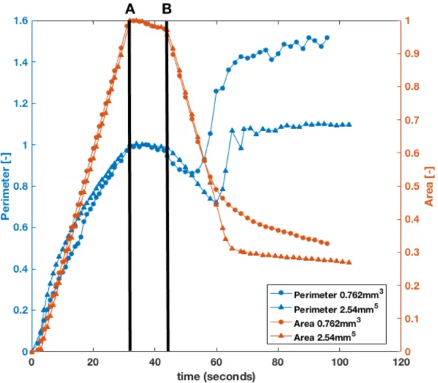
Fig. 2 (A, B, C, D) Concentration maps for two XG experiments with an aperture of 2.54mm and
a flow rate of 20mL/min (A and B), and with an aperture of 0.762mm and a flow rate of 20 mL/min (C and D). The white line in all four images represents a 20mm length scale. (A) and
(C) show the injection phase (viscously-stable displacement), while (B) and (D) illustrate the
withdrawal phase (viscously unstable displacement). The white box in (A) shows a magnification of the mixing zone and the white box in (C) shows a magnification of the
unexpected mixing fringe (within the mixing zone), which was observed at high shear. The black box in (B) outlines a viscous finger (VF) as it formed toward the withdrawal site. A film of XG and stationary regions of XG were also observed and are indicated by the white arrows
Fig. 3 Width of the mixing zone region normalized by the total radius of the space occupied by
the injected fluid, plotted as a function of the volume of injected fluid for four experiments. The 20 mL/min flow rate with a 0.762m aperture experiment (orange triangles) and the 5 mL/min flow rate with a 0.762mm aperture experiment (orange circles) had a mixing fringe present. The other two experiments, 20 mL/min flow rate with a 1.27mm aperture experiment (blue triangles) and the 5mL/min flow rate with a 1.27mm aperture experiment (blue circles) had no mixing fringe present. Even though the experiments had entirely different mixing zone processes, the mixing zone width grew at a similar rate for all experiments
Fig. 4 Mixing zone phase diagram for flow rate and aperture. The size of the data point
corresponds to the area of the mixing zone, normalized by the total area of the XG. The color of the data point corresponds to the spatial autocorrelation of concentration values in the mixing zone. Each experiment has a corresponding number, which is referenced as superscripts in later figures. A mixing zone was observed in all experiments. The mixing fringe is indicated by areas of high spatial autocorrelation, which are color coded as yellow in this diagram. The mixing fringe is a function of both aperture and flow rate. A marked mixing fringe was observed in experiments with a high flow rate and small aperture
Fig. 5 Concentration maps at the end of the injection phase and during the withdrawal phase for
various experiments. The white line in each image represents a 20mm reference scale. The number in the upper right corner of each image is the experiment number referenced in the phase diagram. (A) experiments with a constant 20 mL/min flow rate and various apertures. (B)
experiments with a constant 0.762 mm aperture and various flow rates. The presence of the mixing fringe is more marked with decreasing aperture and increasing volumetric flow rate
Fig. 6 Spatial Autocorrelation as a function of the ratio of the flow rate to the aperture. The size
of the symbol corresponds to the area of the mixing zone normalized by the total invaded area, and the color corresponds to the aperture
Fig. 7 Spatial Autocorrelation as a function of the width of the mixing zone. The size of the
Fig. 8 Contour maps of concentration values of XG for two experiments with the following
aperture and volumetric flow rate: 1.27mm and 10 ml/min (A) and 0.762mm and 20 ml/min (B). The black line in both A and B represents a 20mm reference scale. The color of the contour indicates the concentration of XG at a given location. In both (A) and (B) the first VF to form is indicated by the black box. The VF in the black box is magnified to better observe the
concentration contours. A mixing fringe was observed at injection in experiment B, but not in experiment A. The concentric lines in B show that a moderate radial gradient in concentration is superimposed to the finger structure, while in A the radial concentration gradient is much more abrupt. The blue contours represent the inner boundary of the resident water invading the VF. The dark red contours (100% XG concentration) represent the outer boundary of the VF
Fig. 9 (A, B) Binary images taken during the withdrawal phase of (A) glycerol and (B) XG
experiments. The white line in both images represents a 20mm reference length. Both experiments had a flow rate of 10 mL/min and 1.27mm aperture. (A) The glycerol interface formed instabilities all across the perimeter while in (B) the XG interface only formed
instabilities in a few locations only due to its shear-thinning behavior. This highlights a major difference in VF formation for miscible Newtonian and non-Newtonian fluids in a radial Hele-Shaw cell
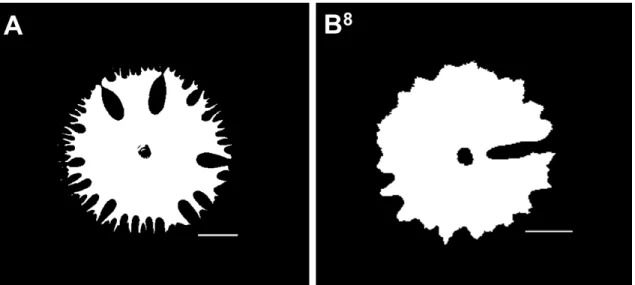
Fig. 10 Normalized perimeter and area data for two experiments with the same flow rate, 20
mL/min, and different apertures of 0.762mm and 2.54mm. The first black vertical line from the left, A, marks the end of the injection phase. The second black vertical line from the left, B, marks the start of the withdrawal phase. There was a time lag between the injection and withdrawal phases due to hysteresis of the syringe pump indicated between lines A and B. At early times after the withdrawal phase started (after line B), the interface advanced toward the injection site while preserving a radial interface, which is indicated by the initial decrease in perimeter. The apparent onset of instability formation is observed when the perimeter switched from decreasing to increasing
Fig. 11 Normalized perimeter and volume of XG in the Hele-Shaw cell during the withdrawal
phase for six experiments. Two experiments have the same flow rate of 3 mL/min and variable apertures of 1.27mm and 0.762mm. Another three experiments have the same flow rate of 20 mL/min and apertures of 2.54mm, 1.27mm, and 0.762mm. The slowest experiment was performed at a flow rate of 0.25 mL/min with an aperture of 0.762mm. The withdrawal phase began with a normalized XG volume and perimeter of 1. The transition from an initial decrease to increase in perimeter indicates the apparent formation of instabilities and is indicated in each experiment by the large data symbol. Instabilities formed earlier for the 3 mL/min experiment (green) than for the 20 mL/min experiment (blue) so less fluid was extracted for the 3 ml/min (green). It is also shown that instabilities formed earlier for smaller apertures when the flow rate was the same
Fig. 12 Experimental and predicted number of fingers formed, as a function of flow rate and
aperture. The color represents the number of fingers formed. The square data points indicate the number of fingers that is approximated from the curve fitted to the experimental data in the inset, i.e., assuming that the number of fingers is mostly dependent on the aperture. The circle data points indicate the actual experimental number of fingers formed.
Fig. 13 VF width comparison of the last interface for 50% and 90% concentration thresholds for
three experiments with 20 ml/min flow rates and apertures of 1.27mm, 0.762mm and 0.508mm. Only VF with both an identified 50% and 90% fingertip were used in this analysis. Each data point represents a finger. The triangle data points indicate the finger from each experiment that reached the injection site first. As expected, the 90% width was greater than the 50% widths. The 50% widths represent the inner water boundary while the 90% widths represent the outer
Fig. 14 Width and length of individual VF for three experiments (same as in Fig.11) with 20
ml/min flow rates and various apertures of 1.27mm, 0.762mm and 0.508mm. Width and length were recorded for both the 50% and 90% concentration thresholds. The dark-shaded symbols represent the 90% concentration thresholds while the light-shaded symbols represent the 50% concentration thresholds. The data points were obtained from the final interface (time) before the first finger reached the injection site.
Funding:
National Science Foundation under Grant No. NSF/EAR1446915. Any opinions, findings, and conclusions or recommendations expressed in this material are those of the author(s) and do not necessarily reflect the views of the National Science Foundation.Conflict of Interest:
the authors declare that they have no conflict of interest.References:
Abdulbaki, M., Huh, C., Sepehrnoori, K., Delshad, M., & Varavei, A. (2014). A critical review on use of polymer microgels for conformance control purposes. Journal of Petroleum
Science and Engineering, 122, 741–753. https://doi.org/10.1016/j.petrol.2014.06.034
Amar, M., & Poiré, E. (1999). Pushing a non-Newtonian fluid in a Hele-Shaw cell: From fingers to needles. Physics of Fluids, 11(7), 1757–1767. https://doi.org/10.1063/1.870041
Bonn, D., Kellay, H., Braunlich, M., Ben Amar, M., & Meunier, J. (1995). Viscous fingering in complex fluids. Physica A, 220, 60–73. https://doi.org/10.1016/0378-4371(95)00114-M Boschan, A., Charette, V. J., Gabbanelli, S., Ippolito, I., & Chertcoff, R. (2003). Tracer
dispersion of non-Newtonian fluids in a Hele-Shaw cell. Physica A: Statistical Mechanics
and Its Applications, 327(1–2), 49–53. https://doi.org/10.1016/S0378-4371(03)00437-0
Brown, E., & Jaeger, H. M. (2014). Shear thickening in concentrated suspensions:
Phenomenology, mechanisms and relations to jamming. Reports on Progress in Physics,
77(4). https://doi.org/10.1088/0034-4885/77/4/046602
Bunton, P. H., Tullier, M. P., Meiburg, E., & Pojman, J. A. (2017). The effect of a crosslinking chemical reaction on pattern formation in viscous fingering of miscible fluids in a Hele-Shaw cell. Chaos, 27(10). https://doi.org/10.1063/1.5001285
Chen, C. Y., Huang, C. W., Wang, L. C., & Miranda, J. A. (2010). Controlling radial fingering patterns in miscible confined flows. Physical Review E - Statistical, Nonlinear, and Soft
Matter Physics, 82(5), 1–8. https://doi.org/10.1103/PhysRevE.82.056308
Chen, J. Den. (1989). Growth of radial viscous fingers in a Hele-Shaw cell. Journal of Fluid
Mechanics, 201, 223–242. https://doi.org/10.1017/S0022112089000911
Chevalier, C., Amar, M. Ben, Bonn, D., & Lindner, A. (2006). Inertial effects on Saffman-Taylor viscous fingering. Journal of Fluid Mechanics, 552, 83–97.
https://doi.org/10.1017/S0022112005008529
Chui, J. Y. Y., De Anna, P., & Juanes, R. (2015). Interface evolution during radial miscible viscous fingering. Physical Review E - Statistical, Nonlinear, and Soft Matter Physics,
92(4), 1–5. https://doi.org/10.1103/PhysRevE.92.041003
Couder, Y., Gerard, N., & Rabaud, M. (1986). Narrow fingers in the Saffman-Taylor instability.
Physcial Review A, 34(6).
CPKelco. (2008). KELTROL® / KELZAN® Xanthan Gum Book 8th edition, 1–28.
Daccord, G., & Nittmann, J. (1986). Radial Viscous Fingers and Diffusion-Limited Aggregation: Fractal Dimension and Growth SItes. Physical Review Letters, 56(4), 336–339.
Dias, E. O., Alvarez-Lacalle, E., Carvalho, M. S., & Miranda, J. A. (2012). Minimization of viscous fluid fingering: A variational scheme for optimal flow rates. Physical Review
Letters, 109(14), 1–5. https://doi.org/10.1103/PhysRevLett.109.144502
Dintzis, F. R., Babcock, G. E., & Tobin, R. (1970). Studies on dilute solutions and dispersions of the polysaccharide from xanthomonas campestris NRRL B-1459. Carbohydrate Research,
13, 257–267.
Fall, A., Huang, N., Bertrand, F., Ovarlez, G., & Bonn, D. (2008). Shear thickening of cornstarch suspensions as a reentrant jamming transition. Physical Review Letters, 100(1).
https://doi.org/10.1103/PhysRevLett.100.018301
Fast, P., Kondic, L., Shelley, M. J., & Palffy-Muhoray, P. (2001). Pattern formation in non-Newtonian Hele-Shaw flow. Physics of Fluids, 13(5), 1191–1212.
https://doi.org/10.1063/1.1359417
Fu, W. J., Jiang, P. K., Zhou, G. M., & Zhao, K. L. (2014). Using Moran’s I and GIS to study the spatial pattern of forest litter carbon density in a subtropical region of southeastern China.
Biogeosciences, 11(8), 2401–2409. https://doi.org/10.5194/bg-11-2401-2014
Gleasure, R. ., & Phillips, C. . (1990). An Experimental Study of Non-Newtonian Polymer Rheology Effects on Oil Recovery and Injectivity. SPE Reservoir Engineering, an Official
Publication of the Society of Petroleum Engineers, 5(4), 481–486.
Gorell, S., & Homsy, G. M. (1983). A theory of the optimal policy of oil recovery by secondary displacement processes. Applied Mathematics, 43(1), 79–98.
Hebeler, F. (2016). Moran’s I version 1.0.0.0, Matlab File Exchange.
https://www.mathworks.com/matlabcentral/fileexchange/13663-moran-s-i
Hele-Shaw, H. (1898). Investigation of the nature of surface resistance of water and of stream-line motion under certain experimental conditions, 21–46.
Lecourtier, J., Chauveteau, G., & Muller, G. (1986). Salt-induced extension and dissociation of a native double-stranded xanthan. Int. J. Biol. Macromol., 8, 306–310.
https://doi.org/10.1016/0141-8130(86)90045-0
Lemaire, E., Levitz, P., Daccord, G., & Van Damme, H. (1991). From viscous fingering to viscoelastic fracturing in colloidal fluids. Physical Review Letters, 67(15), 2009–2012. https://doi.org/10.1103/PhysRevLett.67.2009
Lindner, A., Bonn, D., Poiré, E. C., Amar, M. Ben, & Meunier, J. (2002). Viscous fingering in non-Newtonian fluids. Journal of Fluid Mechanics, 469, 237–256.
https://doi.org/10.1017/S0022112002001714
Lovoll, G., Meheust Y., Maloy K.J., Aker, E., Schmittbuhl, J. (2005) Competition of gravity, capillary fluctuations and dissipation forces during drainage in a two dimensional porous medium, a pore-scale study. Energy, the International Journal, 30(6) 861-872
Malhotra, S., Sharma, M. M., & Lehman, E. R. (2015). Experimental study of the growth of mixing zone in miscible viscous fingering. Physics of Fluids, 27(1).
https://doi.org/10.1063/1.4905581
Martel, R., Hébert, A., Lefebvre, R., Gélinas, P., & Gabriel, U. (2004). Displacement and sweep efficiencies in a DNAPL recovery test using micellar and polymer solutions injected in a five-spot pattern. Journal of Contaminant Hydrology, 75(1–2), 1–29.
https://doi.org/10.1016/j.jconhyd.2004.03.007
Measurement Specialities, MS5803-02BA Miniature Altimeter Module Datasheet.
https://www.te.com/commerce/DocumentDelivery/DDEController?Action=srchrtrv&DocNm=MS5803-02BA&DocType=Data+Sheet&DocLang=English, 2017 (accessed 1.30.19)
Meheust, Y., Lovoll, G., Maloy, K.J., Schmittbuhl, J.(2002). Interface scaling in a
two-dimensional poros medium under combined viscous, gravity, and capillary effects. Physical
Review. E, 66, 051603.
Mezger, T. (2014). Applied Reology (2nd ed.). Austria: Anton Paar GmbH.
Miranda, J. A., & Widom, M. (1998). Radial fingering in a Hele-Shaw cell: a weakly nonlinear analysis. Physica D, 120, 315–328.
Mishra, M., Trevelyan, P. M. J., Almarcha, C., & De Wit, A. (2010). Influence of double diffusive effects on miscible viscous fingering. Physical Review Letters, 105(20), 2–5. https://doi.org/10.1103/PhysRevLett.105.204501
Obernauer, S., Drazer, G., & Rosen, M. (2000). Stable – unstable crossover in non-Newtonian radial Hele – Shaw flow, 283, 187–192.
Paterson, L. (1985). Fingering with miscible fluids in a Hele Shaw cell. Physics of Fluids, 28(1), 26–30. https://doi.org/10.1063/1.865195
Pons, M.-N., Weisser, E. M., Vivier, H., & Boger, D. V. (1999). Characterization of viscous fingering in a radial Hele-Shaw cell by image analysis. Experiments in Fluids, 26(1–2), 153–160. https://doi.org/10.1007/s003480050274
Rodd, A. B., Dunstan, D. E., & Boger, D. V. (2000). Characterization of xanthan gum solutions using dynamic light scattering and rheology. Carbohydrate Polymers, 42(2), 159–174. https://doi.org/10.1016/S0144-8617(99)00156-3
Sader, J. E., Chan, D. Y. C., & Hughes, B. D. (1994). Non-Newtonian effects on immiscible viscous fingering in a radial Hele-Shaw cell. Physical Review E, 49(1), 420–433.
Saffman, P. G., & Taylor, G. I. (1958). The penetration of a fluid into a porous medium or Hele-Shaw cell containing a more viscous liquid. Proc. R. London Ser, 245, 312–329.
Sumner, R. (2014). Processing RAW Images in MATLAB. Retrieved from https://rcsumner.net/raw_guide/RAWguide.pdf
Swann, B. (2017). Leveraging fluids with weak yield stress for directed alignment and distribution of magnetic disks in novel inks. (Masters thesis, Oregon State University, Corvallis, USA)
Thomé, H., Rabaud, M., Hakim, V., & Couder, Y. (1989). The Saffman-Taylor instability: From the linear to the circular geometry. Physics of Fluids A, 1(2), 224–240.
https://doi.org/10.1063/1.857493
Tosco, T., & Sethi, R. (2010). Transport of non-Newtonian suspensions of highly concentrated micro and nanoscale iron particles in porous media: a modeling approach. Environmental
Science and Technology, 44(23), 9062–9068.
Toussaint, R., Måløy, K. J., Méheust, Y., Løvoll, G., Jankov, M., Schäfer, G., & Schmittbuhl, J. (2012). Two-Phase Flow: Structure, Upscaling, and Consequences for Macroscopic
Transport Properties. Vadose Zone Journal, 11(3). https://doi.org/10.2136/vzj2011.0123 White, A. R., & Ward, T. (2014). Constant pressure gas-driven displacement of a shear-thinning
liquid in a partially filled radial Hele-Shaw cell: Thin films, bursting and instability. Journal
of Non-Newtonian Fluid Mechanics, 206, 18–28.
https://doi.org/10.1016/j.jnnfm.2014.02.002
Yang, Z., Méheust, Y., Neuweiler, I., Hu, R., Niemi, A., & Chen, Y.-F. (2019). Modeling immiscible two-phase flow in rough fractures from capillary to viscous fingering. Water
Resources Research, 2033–2056. https://doi.org/10.1029/2018WR024045
Zhong, L., Oostrom, M., Truex, M. J., Vermeul, V. R., & Szecsody, J. E. (2013). Rheological behavior of xanthan gum solution related to shear thinning fluid delivery for subsurface remediation. Journal of Hazardous Materials, 244–245, 160–170.