HAL Id: hal-01698477
https://hal.archives-ouvertes.fr/hal-01698477
Submitted on 31 Oct 2020
HAL is a multi-disciplinary open access
archive for the deposit and dissemination of
sci-entific research documents, whether they are
pub-lished or not. The documents may come from
teaching and research institutions in France or
abroad, or from public or private research centers.
L’archive ouverte pluridisciplinaire HAL, est
destinée au dépôt et à la diffusion de documents
scientifiques de niveau recherche, publiés ou non,
émanant des établissements d’enseignement et de
recherche français ou étrangers, des laboratoires
publics ou privés.
Distributed under a Creative Commons Attribution - NoDerivatives| 4.0 International
users to flash flood events
Saif Shabou, Isabelle Ruin, Céline Lutoff, Samuel Debionne, Sandrine
Anquetin, Jean-Dominique Creutin, Xavier Beaufils
To cite this version:
Saif Shabou, Isabelle Ruin, Céline Lutoff, Samuel Debionne, Sandrine Anquetin, et al.. MobRISK: a
model for assessing the exposure of road users to flash flood events. Natural Hazards and Earth System
Sciences, European Geosciences Union, 2017, 17 (9), pp.1631 - 1651. �10.5194/nhess-17-1631-2017�.
�hal-01698477�
https://doi.org/10.5194/nhess-17-1631-2017 © Author(s) 2017. This work is distributed under the Creative Commons Attribution 3.0 License.
MobRISK: a model for assessing the exposure of road users
to flash flood events
Saif Shabou1, Isabelle Ruin1, Céline Lutoff2, Samuel Debionne1, Sandrine Anquetin1, Jean-Dominique Creutin1, and
Xavier Beaufils1
1Université Grenoble Alpes, CNRS, IGE, 38000 Grenoble, France
2Université Grenoble Alpes, CNRS, PACTE, 38000 Grenoble, France
Correspondence to:Isabelle Ruin ([email protected])
Received: 10 January 2017 – Discussion started: 14 March 2017
Revised: 17 July 2017 – Accepted: 11 August 2017 – Published: 25 September 2017
Abstract. Recent flash flood impact studies highlight that road networks are often disrupted due to adverse weather and flash flood events. Road users are thus particularly exposed to road flooding during their daily mobility. Previous exposure studies, however, do not take into consideration population mobility. Recent advances in transportation research provide an appropriate framework for simulating individual travel-activity patterns using an travel-activity-based approach. These activity-based mobility models enable the prediction of the sequence of activities performed by individuals and locating them with a high spatial–temporal resolution. This paper de-scribes the development of the MobRISK microsimulation system: a model for assessing the exposure of road users to extreme hydrometeorological events. MobRISK aims at providing an accurate spatiotemporal exposure assessment by integrating travel-activity behaviors and mobility adtation with respect to weather disruptions. The model is ap-plied in a flash-flood-prone area in southern France to as-sess motorists’ exposure to the September 2002 flash flood event. The results show that risk of flooding mainly occurs in principal road links with considerable traffic load. How-ever, a lag time between the timing of the road submersion and persons crossing these roads contributes to reducing the potential vehicle-related fatal accidents. It is also found that sociodemographic variables have a significant effect on indi-vidual exposure. Thus, the proposed model demonstrates the benefits of considering spatiotemporal dynamics of popula-tion exposure to flash floods and presents an important im-provement in exposure assessment methods. Such improved characterization of road user exposures can present valuable information for flood risk management services.
1 Introduction
Flash flooding is considered one of the most dangerous natu-ral hazard in terms of human losses. The rapidness and sud-denness of this hydrometeorological phenomenon makes it hardly predictable and decreases the efficiency of rescue op-erations and the available time for people to protect them-selves and to adapt their daily activities and mobility behav-iors. Therefore, several vehicle-related accidents occur dur-ing flash floods. Death circumstances investigations showed that in postindustrial countries over half of flood victims are motorists trapped by road flooding (Ashley and Ashley, 2007; Sharif et al., 2012; Terti et al., 2017). Hence, daily mo-bility is pointed out as one of the primary causes of popula-tion exposure and vulnerability to flash floods (Ruin, 2010). However, mobility aspects are not systematically included in studies assessing human exposure and vulnerability to natural hazards. In order to integrate social vulnerability in risk measurement, population density data is often used as-suming a static distribution, which contrasts with the fast dynamics of the flash flood phenomenon. Recently, it has progressively been acknowledged that variation of popula-tion distribupopula-tion may provide a more accurate assessment of human exposure to natural hazards. Aubrecht et al. (2012) stressed the importance of including temporal variations of social vulnerability in every phase of the disaster manage-ment cycle. For instance, Freire and Aubrecht (2012) con-sidered nighttime- and daytime-specific population densities for assessing population exposure to earthquake hazard in the Lisbon Metropolitan Area. Results showed that people are potentially at risk in the daytime period. In the context of flash floods, Terti et al. (2015, 2017) and Spitalar et al. (2014) showed that daily and sub-daily variation of population
dis-tribution may provide an appropriate assessment of human exposure to such short-fuse weather events.
In fact, motorists’ exposure to flood events is directly re-lated to disruption and degradation of the road network. Road network studies use graph theory and more specifically di-rected graphs (called network) where the so-called edges or arcs represent the road segments linking the nodes or ver-tices corresponding to the road intersections. Several stud-ies in transportation research focused on road network vul-nerability to adverse weather conditions (Koetse and Ri-etveld, 2009; Transportation Research Board, 2008). Dif-ferent methods were developed in order to identify critical road segments where disruptions would lead to severe conse-quences. Berdica (2002) defined road segment vulnerability as a function of the probability of occurrence of hazardous events and the importance of related impacts in terms of ser-viceability of road links. Jenelius et al. (2006) quantified the road network vulnerability by introducing the concept of crit-icality of the network constituents (e.g., link, node, groups of links and/or nodes), which includes both the probability of the constituents failing and the consequences of that fail-ure for the system as a whole. Link criticalities depend on their weakness and their importance for the functioning of the whole network measured by the increased generalized travel cost when these links are closed.
Recently, Versini et al. (2010a) proposed a method for assessing road susceptibility to flooding in the Gard region (France) based on an inventory of observed flooded road sec-tions over the last 40 years. The risk of road flooding is com-puted by combining susceptibility to flooding on a given road with simulated stream discharge of the corresponding river segment (Versini et al., 2010b). Naulin et al. (2013) extended the road flooding forecasting tool to the entire Gard region and proposed a method for allocating probabilities of flood-ing to road–river intersections (called “road cuts”) depend-ing on return periods of stream discharges (Naulin, 2012). Versini and Naulin’s studies contribute to better forecasting the chance of road flooding, hence providing a strong base to further analyze the impact of road users’ exposure.
To consider the risk for mobile people during flash flood there is a need to integrate travel-activity behaviors and indi-vidual responses to weather disruptions. Recently, impacts of extreme weather events on traffic flow and travel behaviors received much attention in transportation research (Böcker et al., 2013; Al Hassan and Barker, 1999; Koetse and Ri-etveld, 2009; Chung et al., 2005). Böcker et al. (2013) pro-vided an extensive literature review on the potential impacts of weather on individual daily travel behaviors such as trip generation, travel destination and mode choices. Tsapakis et al. (2013) showed that high intensity of snow and rain de-creases travel speed and inde-creases travel time in the Greater London area. They also found that the impacts of weather conditions largely depend on drivers’ attitudes, socioeco-nomic characteristics and other contextual factors. Andrey et al. (2013) investigated the effect of exposure frequency to
adverse weather conditions on drivers’ adaptation behaviors and concluded that drivers do not tend to acclimatize to lo-cal weather patterns. Based on a survey on travel decisions, Khattak and De Palma (1997) showed that adverse weather has a strong impact on travel decision changes such as route choice, transport mode choice and departure time.
These decisions partly depend on individual risk percep-tion and personal evaluapercep-tion of the environmental threat, which largely vary between individuals. Ruin et al. (2007) examined the effects of sociodemographic characteristics on perceived risk related to driving under heavy rain and through flooded roads. It was found that young male drivers have a clear tendency to underestimate the corresponding risk. Other factors seem to have a significant effect on mobil-ity adaptation to flood events such as flood danger knowl-edge, flooding experience and route familiarity (Drobot et al., 2007; Ruin et al., 2009). In addition to risk perception, daily constraints related to professional and family activities are strong drivers of mobility regardless of the weather con-ditions (Ruin et al., 2007, 2014). The perceived importance and flexibility of planned and scheduled activities might play an important role in mobility adaptation capacities. Cools et al. (2010) demonstrated that travel change decisions related to weather conditions depend on trip purposes, with leisure and shopping activities being more likely to be canceled and postponed than work or school activities.
Thus, these findings highlight the relevance of considering both individual sociodemographic characteristics and daily activity schedules and constraints to establish an accurate as-sessment of population exposure to road flooding. Recent ad-vances in mobility modeling following an activity-based ap-proach offer an appropriate framework to microsimulate in-dividual travel-activity patterns (Rasouli and Timmermans, 2014). These activity-based models consider travel behavior as derived from the demand of activity participation and aim at predicting the sequence of activities conducted by individ-uals (McNally, 1995). Activity-based models gain increasing interest in dynamic exposure assessment research, which is especially illustrated in air pollution exposure studies (Beckx et al., 2008, 2009; Pebesma et al., 2013) and homeland secu-rity applications (Henson et al., 2009). Flood exposure stud-ies can also benefit from the wealth of information provided by this kind of mobility modeling approach. Indeed, the com-bination of individual travel-activity simulations with road flooding forecasts makes a thorough assessment of motorists’ exposure and their evolution in time and space regarding the flood hazard possible.
In this paper we present the so-called MobRISK model, which aims at providing an assessment of motorists’ expo-sure to flash floods by taking into account travel-activity behaviors and mobility adaptation with respect to weather disruptions and roads flooding. MobRISK is considered a microsimulation system since each individual of the popu-lation is represented individually, similarly to agent-based models (Gilbert, 2007). It is also an activity-based
mobil-ity model in which the full individual travel-activmobil-ity pat-terns are simulated. We illustrate the potential benefits of the proposed model through an application of MobRISK in the Gard region, which is a flash-flood-prone administrative area (French department) located in southern France. The objec-tive of the proposed case study is to quantify motorists’ expo-sure to the 8–9 September 2002 major flash flood event that resulting in 24 victims in the Gard area.
The remainder of the paper is organized as follows. The next section describes the conceptual modeling approach used in the MobRISK model. Section 3 details the required input data together with the description of the individual ex-posure measurement method. The case study area and results from MobRISK simulations are illustrated in Sect. 4. Finally, Sect. 5 discusses the results and provides insights for further research and potential improvements of the model.
2 MobRISK modeling approach
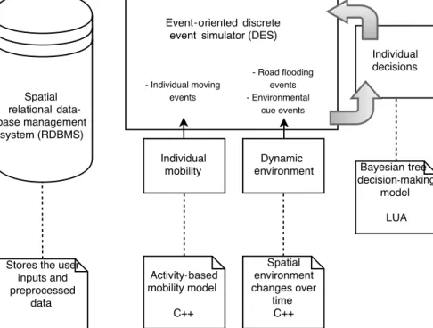
MobRISK is a model for assessing and simulating road users’ exposure to road flooding due to extreme flash flood events by combining travel-activity simulations following an activity-based approach with hydrometeorological data. The MobRISK architecture includes (i) the simulated environ-mental changes considered for the study such as road flood-ing, (ii) an activity-based mobility model reproducing pop-ulation travel-activity behaviors and (iii) a decision-making model predicting individual responses to weather disrup-tions. A discrete event simulator (DES) runs the main tem-poral loop of the simulations. In addition, the user input data is stored in a spatial relational database management system (Fig. 1).
2.1 Discrete event simulation
The core of the MobRISK simulator is a parallel discrete event simulator that runs the main temporal loop of the simu-lation. The pending event set is organized as a priority queue, sorted by event time and therefore handled in chronological order (Fujimoto, 1999; Robinson, 2004). Event-driven sim-ulations are efficient in terms of computation time as they avoid unnecessary time steps. Four types of events are han-dled in MobRISK:
– road flooding: records different changes in probabilities of road flooding during a simulation period;
– environmental cue: reports the changes in environment and weather conditions that might be perceived by indi-viduals such as precipitation intensities;
– broadcast: contains diverse warning and alert informa-tion that can be received by individuals and may affect their travel decisions; and
– travel activity: records changes of individual locations (at the road nodes resolution) and the travel purposes.
2.2 Mobility modeling
As explained in Sect. 1, to better understand and analyze mo-bility behaviors under environmental perturbations, we need to integrate daily travel motivations in the mobility modeling. Following an activity-based approach for mobility modeling, travel demand is considered to derive from the human need to perform different activities distributed in time and space (Recker et al., 1986). Recently, activity-based models have been gaining increasing attention due to the wealth of infor-mation they provide and the incorporation of behavioral and psychological components and decision-making processes.
The activity-based approach in travel modeling emerged in the 1970s as a complement to the concept of time geography of Hägerstrand (1970) and Chapin (1974), which introduced the importance of various spatial and temporal constraints on individuals’ mobility behavior. While classical trip-based models, commonly referred to as “four step models”, are fo-cusing essentially on the quantification of trips generated by population mobility without considering the sequential char-acteristics and the behavioral dimension, activity-based mod-els aim at predicting how, why, when, how often, where and with whom the different activities are conducted by the indi-viduals (Bhat and Koppelman, 1999). McNally (1995) iden-tified the most important specificities of activity-based mod-eling: (i) travel is derived from the demand for activity partic-ipation; (ii) sequences and patterns of travel behavior are the units of analysis instead of individual trips in trip-based mod-els; (iii) household and sociodemographic characteristics af-fect travel-activity behavior; and (iv) spatial, temporal and in-terpersonal factors that constrain travel-activity patterns are taken into account.
Over the last years, several activity-based models have been developed: TRANSIMS (Smith et al., 1995), ALBA-TROSS (Arentze and Timmermans, 2000), CEMDAP (Bhat et al., 2004), MATSim (Balmer et al., 2006) and ADAPTS (Auld and Mohammadian, 2009). Although the mentioned models follow the same activity-based paradigm and provide useful frameworks for modeling individual motilities, they have some differences regarding the activity scheduling ap-proach used, the decision-making process integration and the required input data structure. These differences depend es-sentially on research purposes and data availability.
Whereas the mentioned models are essentially applied for transport forecasting and urban planning, the main objective of MobRISK is to assess population mobility exposure to road flooding, which requires the combination of the travel-activity simulation with hydrometeorological data and road flooding impact data. Census data and travel-activity survey data are needed in order to assign daily activity programs to the population. Then, by locating the different activity ar-eas, the population mobility is generated when individuals at-tempt to implement their activity programs. Finally, individ-ual exposure over the flash flood event is defined by the
prob-Figure 1. The MobRISK model architecture includes (i) the simulated environmental changes considered for the study such as road flooding, (ii) an activity-based mobility model reproducing population travel-activity behaviors and (iii) a decision-making model predicting individual responses to weather disruptions. A discrete event simulator (DES) runs the main temporal loop of the simulations. In addition, the user input data is stored in a spatial relational database management system.
ability (given the location and timing) of crossing flooded roads along each individual’s route.
3 Data and methods
The MobRISK microsimulator was developed to measure the exposure of inhabitants and people working in the Gard ad-ministrative area, a region of southern France that has a long flash flood history. This region is characterized by a typical Mediterranean climate with heavy rainfall events during the autumn season (Delrieu et al., 2005; Gaume et al., 2009). In fact, since 1225, the Gard region suffered 506 floods. A total of 66 % of the 353 municipalities experienced at least 10 ref-erenced flood events and some of them were affected more than hundreds of times (CG30, 2016). Between 1316 and 1999, Antoine et al. (2001) recorded 27 fatal flood episodes and 277 deaths in Gard. Since 1999, five fatal events added about 30 casualties to the toll. In 2015, nearly 65 % of the businesses and 35 % of the population of the Gard area were located in a flood-prone zone.
In 2010, 726 783 inhabitants were living in the Gard
ad-ministrative area, which has a surface of 5852 km2. Among
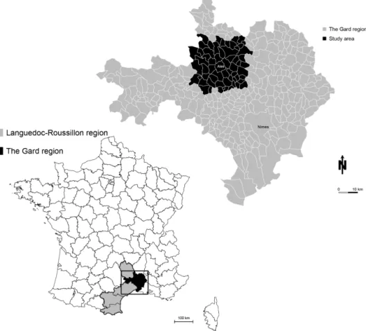
the 353 municipalities, 267 are essentially rural. Urban areas are mostly located next to Nîmes, the capital of the depart-ment consisting of 145 501 inhabitants, and Alès (41 118 in-habitants; Fig. 2). The road network of the Gard region amounts to 12 322 km of roads likely taken by commuters
(paved roads), distributed between local roads (83.8 %), prin-cipal roads (4.8 %), regional roads (10.3 %) and highways (1.1 %). The river network is composed of 6443 river sections totaling 7087 km in length. Based on the work of Versini et al. (2010), a total of 1970 potential road cuts, which would be called “low-water crossing” in the USA, have been iden-tified based on road–river intersections that are sensitive to flooding (see the detailed description in Sect. 3.2; Debionne et al., 2016). Even though the points exposed to flooding may be of three distinct types: river crossings, low accumulation points and river-adjacent points. Low-accumulation points and river-bordering points are much more difficult to iden-tify as they are mostly due to very local settings that are not detectable on the digital terrain model (Versini et al., 2010). Therefore, those two types were not considered in Versini’s work or in the study presented in this paper.
This section provides an overview of the required input data used in the MobRISK model. MobRISK makes max-imum use of existing national databases, both geographi-cal and social. SpatiaLiTE, the spatial extension of SQLiTe (a free relational database management system contained in the C programming library), is used extensively for input database building and preprocessing. The goal of input data preprocessing is to (i) identify the sociodemographic charac-teristics of individuals and households corresponding to the study area, (ii) attribute daily schedules to every individual and (iii) locate the areas where they are likely to conduct
Figure 2. Maps of the study area with (i) the location of the Gard department (black) within the Languedoc-Roussillon region (grey) in France and (ii) the location of the 61 municipalities of the case study area among the 353 municipalities of the Gard department. Source: compiled by author from BD TOPO for regions’ and municipalities’ boundaries (http://professionnels.ign.fr/bdtopo).
their activities. Concerning the geographical data, road and river network data are used for identifying the vulnerability of road sections to flooding.
3.1 Population data
Sociodemographic description of the population is based on census data provided by Insee in 2010 (French National Institute of Statistics and Economic Studies). We use es-pecially the INDCVI dataset, which contains the descrip-tion of sociodemographic characteristics of the individuals, their household composition and household geographical lo-cation at the municipality resolution. In addition, we com-bine MOBPRO (professional mobility) and MOBSCO (stu-dent mobility) datasets issued from the Insee complementary exploration of census data. In addition to individual sociomographics and household characteristics, these datasets de-scribe individuals’ commuting patterns. They include in-formation about the municipalities of residence, work and school activities, traveled distances and usual commuting modes of professionals in five categories: (1) no transport; (2) on foot; (3) two-wheel vehicle; (4) car, truck and van; and (5) public transport. These data are stored into
“individ-ual” and “household” tables and every individual is assigned to one household.
The description of individual activity schedules is based on travel-activity data, provided by the French National Transport and Travel Survey (ENTD) carried out by Insee from 2007 to 2008. In this survey, the responders were asked to indicate their sociodemographic characteristics (age, gen-der, professional status, etc.), their household composition and their mobility description during 1 weekday and 1 week-end. They were instructed to mention the different trips they made during the days of the survey, transport modes, trips’ purposes, and time of departure and arrival. Based on these data, the individuals’ schedules were retrieved, representing a sequence of activities mentioned by responders as trip pur-poses. Ten main activities are proposed in the survey: home, school, working, shopping, medical appointment, adminis-trative procedure, visiting, accompanying persons, leisure and holiday activities.
The main objective of using the ENTD data is to assign daily schedules to the individuals described by the census data based on the effects of sociodemographic variables on schedules dissimilarities. The dissimilarities between
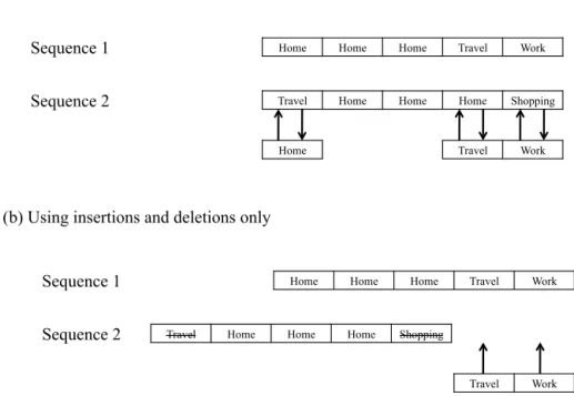
sched-ules and pairs of sequences are measured by counting the number and type of operations needed to transform one se-quence into the other (to match them). The operations con-sidered are insertions, deletions or substitutions of activities. Figure 3 illustrates the matching of a pair of sequences in two different ways regarding the type of operation: (i) us-ing only substitutions by replacus-ing the different elements of one sequence with those in the second one and (ii) using a combination of insertion and deletion operations. The opti-mal matching (OM) distance metric allowing both substitu-tions and insertion/deletion of activities (Lesnard et al., 2011) is used in this study. Moreover, a method proposed by Studer et al. (2011) called the “discrepancy analysis” allows mea-suring the relationships between categorical variables (e.g., gender, age, education level, professional status) and a set of sequences described by the matrix of dissimilarities (mea-sured with the OM method). It consists of measuring the pair-wise dissimilarities between different activity sequences and implementing an ANOVA test to identify sociodemographic variables that explain the discrepancy of the sequences.
In addition to measuring the effect of sociodemographic variables on sequence dissimilarities, Studer et al. (2010, 2011) proposed a complementary regression tree analysis, which consists of a recursive partitioning of the sequences based on splitting criteria derived from the dissimilarity anal-ysis. All individual activity sequences are grouped in the first node of the tree (root node). A discrepancy analysis is dis-played to identify the variable explaining the greatest part of the sequence discrepancies. The sequences are then par-titioned based on this variable in such a way that the
result-ing child1nodes are as homogeneous as possible (with a low
within dissimilarity). This operation is repeated recursively until no significant effect of sociodemographic variables is registered in the nodes’ sequences. Hence, the schedule at-tribution rules can be extracted from the obtained tree with respect to the strength of relationships between sociodemo-graphic characteristics and activity sequences. Then, every individual in the study area is connected to an average week schedule and an average weekend schedule based on these attribution rules. The proposed framework is implemented into a free package in R software called TraMineR (Gabad-inho et al., 2011). Sequence discrepancy analysis methods have been especially used for exploring individual life tra-jectories (Studer et al., 2010; Widmer and Ritscard, 2009). Recent applications of sequence analysis methods on activ-ity schedules and diary data have revealed the advantages of these approaches for capturing the complex structures of ac-tivity patterns and providing more accurate schedule classifi-cations (Lesnard and Kan, 2011; Kim, 2014).
1A child node is a node directly connected to another node when
moving away from the root node of the tree.
3.2 Geographical data
The next step in preprocessing the data for activity-based mo-bility modeling consists of locating the different areas where individuals might conduct their activities. Concerning hous-ing activities, census data provide the municipality of resi-dency of every household. In order to have a more precise spatial resolution, we use the RFL data (Revenus Fiscaux lo-calisés – household localized taxes) published by Insee in 2010. The RFL data concerns the number of households and individuals living in them and their sociodemographic de-scription provided at 200 m × 200 m resolution for the en-tire French territory. Then, each household is located in the grid with respect to household densities by pixel. Concern-ing work and school activities, MOBPRO and MOBSCO datasets provide the municipalities’ codes of both work and school places for workers and students. In order to enhance the spatial resolution, work and school places are assumed to be mostly located close to municipalities’ administrative cen-ters. Therefore, we assign a road node inside a buffer with a radius of 200 m around administrative centers of work and school municipalities to every worker and student. Finally, since we do not have reliable data for the locations of other activities (shopping, leisure, visiting, etc.), we randomly as-sign a road node inside a buffer of 500 m around the adminis-trative center of every individual’s municipality of residency. The road network sensitivity to flooding is based on the connection of three datasets providing the description of the road and river networks and a list of the road sections sus-ceptible to flooding called road cuts. Road network data is
provided in the BD CARTO®database by the IGN (French
National Mapping Agency), describing the road segments that compose the entire French road network by specify-ing their characteristics (regional, principal or local roads) and their locations in 2010. The second geographic infor-mation layer used refers to the river network provided by
the BD CARTHAGE® database. It contains the different
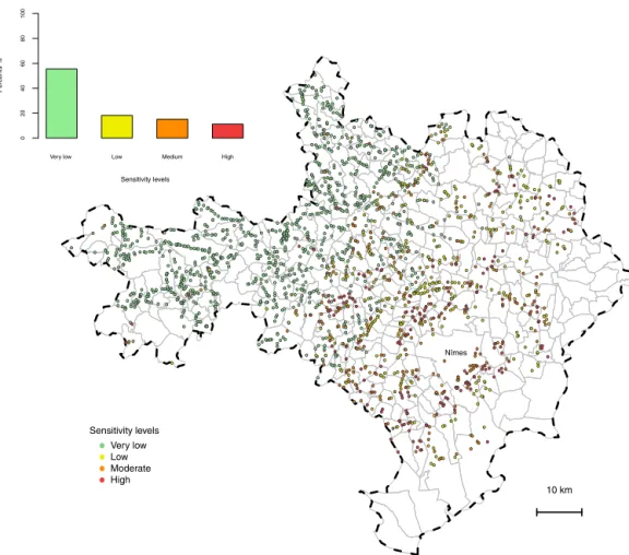
hydrographic segments and their attributes. The road cuts (low water crossings) dataset is derived from the intersec-tion of river and road networks and calibrated using an in-ventory of road flooding during the last 40 years provided by the Gard road management services. Based on this dataset, Versini et al. (2010a) identified 1970 road cuts in the Gard road network and produced a classification of these road sec-tions according to their susceptibility to flooding (Fig. 4).
The four susceptibility classes range from s0to s3,
measur-ing 1093, 359, 297 and 221 points respectively. The “very
low” susceptibility to flooding class s0corresponds to road–
river intersections that have empirical return periods of
flood-ing exceedflood-ing 40 years. The “weak” s1, “medium” s2 and
“high” s3 susceptibility classes have an empirical flooding
return period smaller than 1 year in 20, 35 and 65 % of their points respectively. Based on road cut classification, Naulin et al. (2013) developed a method to compute a probability of submersion for each road cut by combining the susceptibility
Home Home Home Travel Work
Travel Home Home Home Shopping
Home Travel Work
( a) Using substitutions only Sequence 1
Sequence 2
Home Home Home Travel Work
Travel Home Home Home Shopping
Travel Work
( b) Using insertions and deletions only Sequence 1
Sequence 2
Figure 3. Schematic representation of sequence-matching operations. This figure illustrates the matching of a pair of sequences in two different ways regarding the type of operation: (a) using only substitutions by replacing the different elements of one sequence with those in the second one and (b) using a combination of insertion and deletion operations.
classes and simulated stream discharges at the section of river responsible for the road cut. Therefore, an interval of prob-ability of submersion is assigned to every road cut for each combination susceptibility class and return period of stream discharge. In order to have one value of probability of sub-mersion, the probability intervals are simplified in this study by considering the average value within interval probability limits (Table 1).
3.3 Route choice and exposure measurement methods
Once the different activities of each individual schedule are located and road section attributes are specified, the route se-lection criteria needs to be defined. Although various factors are involved in the route choice process, several studies in-dicated that minimizing travel time is the principal criterion for selecting routes (Papinski et al., 2009; Ramming, 2002; Bekhor et al., 2006). Therefore, we chose to use the classical Dijkstra algorithm – a single source shortest path algorithm that provides trees of minimal total length and time in a con-nected set of nodes (Dijkstra, 1959). The activity pattern at-tributions concern only the starting times and durations of the activities’ sequences, which means that travel duration is computed based on the distance between the different activ-ity locations for each individual. Therefore, the implemented schedules may be distorted compared to the assigned ones in terms of travel durations. Finally, motorists’ exposure to road submersion can be measured based on the probability to encounter one or several flooded road cuts on their route
during the simulated event period. The more important the probability of crossing submerged road cuts is, the higher the individual exposure is. Since individuals are likely to cross several road cuts with different probabilities of submersion, total exposure is computed by calculating the joint probabil-ity of submersion of all the crossed road cuts. The individual exposure index is calculated with the following Eq. (1):
E(ind) = 1 −Y
k
(1 − P (Subk)), (1)
where E(ind) refers to the computed individual exposure and
P(Subk)is the probability of submersion in the kth road cut
crossed. An example of exposure measurement is illustrated and explained in Fig. 5.
4 Results
Even though MobRISK model development is at the scale of the Gard department, we present in this section a first appli-cation of the model in the subregion of Alès located in the north of the Gard administrative area (Fig. 2).
4.1 Case study
The objective of this case study is to assess road users’ expo-sure to road flooding during the 8–9 September 2002 event, which is considered to be one of the most catastrophic flash floods in the area since the one from 1958. In this first
ap-Very low Low Medium High
Percents of sensitivity levels of road cuts
Sensitivity levels Percents % 0 20 40 60 80 100 ● ● ● ● ● ● ● ● ● ● ● ● ● ●● ● ● ● ● ● ● ● ● ● ● ● ● ● ● ● ● ● ● ● ● ● ● ● ● ● ●● ● ● ● ● ● ● ● ● ● ● ● ● ● ● ● ● ● ● ● ● ● ● ● ● ● ●● ● ● ● ● ● ● ● ● ● ● ● ● ● ● ●● ● ● ● ● ● ● ● ● ● ● ● ● ● ● ● ● ● ● ● ● ● ● ● ● ● ● ● ● ● ● ● ● ● ● ● ● ● ●● ● ● ● ● ● ● ● ● ● ● ● ● ● ● ● ● ● ● ● ● ● ● ● ● ● ● ● ● ● ●●● ● ● ● ● ●● ● ● ● ● ● ● ● ● ● ● ● ● ● ● ● ● ● ● ● ● ● ● ● ● ● ● ● ● ● ● ● ● ● ● ●●● ●● ● ● ● ● ● ● ● ● ● ●●● ● ● ● ● ● ● ● ● ● ● ● ● ● ● ● ● ● ● ● ● ● ● ● ● ● ● ● ● ● ● ● ● ● ● ● ● ● ● ● ● ● ● ● ● ● ● ● ● ● ●● ● ● ●● ● ● ● ● ● ● ● ● ● ●● ● ● ● ● ● ● ● ● ● ● ● ● ● ● ● ● ● ● ● ● ● ● ● ● ●● ● ● ● ● ● ● ● ● ● ● ● ● ● ● ● ● ● ● ● ● ● ● ● ● ●● ● ● ● ● ● ● ● ● ● ● ●● ● ● ● ● ● ● ● ● ● ● ● ● ● ● ● ● ● ● ● ● ● ● ● ● ● ●● ● ● ● ● ● ● ● ● ● ● ● ● ● ● ● ● ● ● ● ● ● ● ● ● ● ● ● ● ● ● ● ● ● ● ● ● ● ● ● ● ● ●● ● ● ● ● ● ● ● ● ● ● ● ● ● ● ● ● ● ● ● ● ● ● ● ●● ● ● ● ● ● ● ● ● ● ● ● ● ● ● ● ● ● ● ● ● ● ● ● ● ● ● ● ● ● ● ● ● ● ● ● ● ● ● ● ● ● ● ● ● ● ● ● ● ● ● ● ● ● ● ● ● ● ● ● ● ● ● ● ● ● ● ● ● ● ●● ● ● ● ● ● ● ● ● ● ● ● ●●● ● ● ●● ● ● ● ● ● ● ● ● ● ● ● ● ● ● ●● ● ● ● ● ● ● ● ● ● ● ● ● ● ●● ● ● ● ● ● ● ●● ● ● ● ● ● ● ● ● ● ●● ● ● ● ● ● ● ● ● ● ● ● ● ● ● ● ● ● ● ● ● ●● ● ● ● ● ● ● ● ● ● ● ● ● ● ● ●● ● ● ● ● ● ● ● ● ● ● ● ● ● ● ●● ● ● ● ● ● ● ● ● ● ● ● ● ● ● ● ● ● ● ● ● ● ● ● ● ● ● ● ● ● ● ● ● ● ● ● ● ● ● ● ● ● ● ● ● ● ● ● ● ● ● ● ● ● ● ● ● ● ● ● ● ● ● ● ● ● ● ● ● ● ● ● ● ● ● ● ● ● ● ● ● ● ● ● ● ● ● ● ●●● ● ● ● ● ● ● ● ● ● ● ● ● ● ● ● ● ● ● ● ● ● ● ● ● ● ● ● ● ● ● ● ● ● ● ● ● ● ● ● ● ● ● ● ● ● ● ● ● ● ● ● ● ● ● ● ● ● ● ● ● ● ● ● ● ● ● ● ● ● ● ● ● ● ● ● ● ● ● ● ● ● ● ● ●● ● ● ● ● ● ● ● ● ● ● ● ● ● ● ● ●●● ● ● ● ● ● ● ● ● ● ● ● ● ● ● ● ● ● ● ● ● ● ● ● ● ● ● ● ● ● ● ● ● ● ● ● ● ● ● ● ● ● ● ● ● ● ● ● ● ● ● ● ● ● ● ●● ● ●● ● ● ● ● ● ● ●● ● ● ● ● ● ● ● ● ● ● ● ● ● ● ● ●● ● ● ● ● ● ● ● ● ● ● ● ● ● ● ● ● ● ● ● ● ●● ● ● ● ● ● ● ●● ● ● ● ● ● ● ● ● ● ● ● ● ●● ● ● ● ● ● ● ● ● ● ● ● ● ● ● ● ● ● ● ● ● ● ● ● ● ● ● ● ● ● ● ● ● ● ● ● ● ● ● ● ● ● ●● ● ● ● ● ● ● ● ● ● ● ● ● ● ● ● ● ● ● ● ● ● ● ● ● ● ● ● ● ● ● ● ● ● ● ● ● ● ● ● ●● ● ● ● ● ● ● ● ● ● ● ● ● ● ● ● ● ● ● ● ● ● ● ● ● ● ● ●●● ● ● ● ● ● ● ● ● ● ● ● ● ● ●●● ● ● ● ● ● ● ● ● ● ● ● ● ● ● ● ●● ● ● ● ● ● ● ● ● ● ● ● ● ● ● ● ● ● ● ● ● ● ● ● ● ● ● ● ● ● ● ● ● ● ● ● ●● ● ● ● ● ● ● ● ● ● ● ● ● ● ● ● ● ● ●● ● ● ● ● ● ● ● ● ● ● ●● ●● ● ● ● ● ● ● ● ● ● ● ● ● ● ● ● ● ● ● ● ● ● ● ● ● ● ● ● ● ● ● ● ● ● ● ● ● ● ● ● ● ● ● ●● ● ● ● ● ● ● ● ● ● ● ● ● ● ●● ● ● ● ● ● ● ● ● ● ● ● ● ● ● ● ● ● ● ● ●● ● ● ● ● ●● ● ● ● ● ● ● ● ● ● ● ● ● ● ● ● ● ● ● ● ● ● ● ● ● ● ● ● ● ● ● ● ● ● ● ●● ● ● ● ● ● ● ● ● ● ● ● ● ● ● ● ● ● ● ● ● ● ● ● ● ● ● ● ● ● ● ● ● ● ● ● ● ● ● ● ● ● ● ● ● ● ● ● ● ● ● ● ● ● ● ● ●● ●● ● ● ● ● ● ● ● ● ● ● ● ● ● ● ● ● ● ● ● ● ● ●● ● ● ● ● ● ● ● ● ● ● ●● ● ●● ● ● ● ● ● ● ● ● ● ● ● ● ● ● ● ● ● ● ● ● ● ● ● ● ● ● ● ● ● ● ● ● ● ● ● ● ● ● ● ● ● ● ● ● ● ● ● ● ● ●●●● ● ● ●● ● ● ● ●● ● ● ● ● ● ● ● ● ● ● ● ● ● ● ● ● ● ● ● ● ●● ● ● ● ● ● ● ● ● ● ●● ● ● ● ● ● ● ● ● ● ● ●● ● ● ● ● ● ● ● ● ● ● ● ● ● ● ● ● ● ● ● ● ● ● ● ● ● ● ● ● ● ● ● ● ● ● ● ● ● ● ● ● ● ● ● ● ● ● ● ● ● ● ● ● ● ● ● ● ● ● ● ● ● ● ● ● ● ● ● ● ● ● ● ● ● ●● ● ● ● ● ● ● ● ● ● ● ● ● ● ● ● ● ● ● ● ● ● ● ● ● ● ● ● ● ● ● ● ● ● ● ● ● ● ● ● ● ● ● ● ● ● ● ● ● ● ● ● ● ● ● ● ● ● ● ● ● ● ● ● ● ● ● ● ● ● ● ● ● ● ● ● ● ● ● ● ● ● ● ● ● ● ● ● ● ● ● ● ● ● ● ● ● ● ● ● ● ● ● ● ● ● ● ● ● ● ● ● ● ● ● ● ● ● ● ● ● ● ● ● ● ● ● ● ● ● ● ● ● ● ● ● ● ● ● ● ● ● ● ● ●● ● ● ● ●● ● ● ● ● ● ● ● ● ● ● ● ● ● ● ● ● ● ● ● ● ● ● ● ● ● ● ● ● ● ● ●● ● ● ● ● ● ● ● ● ● ● ● ●● ●● ● ● ● ● ●● ● ● ● ● ●● ● ● ● ● ● ● ● ●● ● ● ● ● ● ● ● ● ● ● ● ● ● ● ● ● ● ● ● ● ● ●●● ● ● ● ● ● ● ● ● ● ● ● ● ● ● ● ● ● ● ● ● ● ● ● ● ● ● ● ● ● ● ● ● ● ● ● ● ● ● ● ● ● ● ● ● ● ● ● ● ● ● ● ● ● ● ● ● ● ● ● ● ● ● ● ● ● ● ● ● ● ● ● ● ● ● ● ● ● ● ● ● ● ● ● ● ● ● ● ● ● ● ● ● ● ● ● ● ● ● ● ● ● ● ● ● ● ● ● ● ● ● ● ● ● ● ● ● ● ● ● ● ● ● ● ● ● ● ● ● ● ● ● ● ● ● ● ● ●● ● ● ● ● ● ● ● ● ● ● ● ● ● ● ● ● ● ● ●● ● ● ● ● ● Sensitivity levels Very low Low Moderate High 10 km Nîmes
Sensitivity levels of road cut points
Figure 4. The spatial distribution of the 1970 road cuts identified in the Gard region with the different flooding susceptibility levels. The top-left bar plot represents the distribution of the road cuts (low water crossings) according to the 4 levels of flooding susceptibility. Source:
compiled by author from BD CARTHAGE®for the hydrographic network (http://professionnels.ign.fr/bdcarthage), BD CARTO®for the
road network (http://professionnels.ign.fr/bdcarto) and Versini et al. (2010a) for the road cut locations and susceptibility levels.
Table 1. Probabilities of submersion of the road cuts depending on the return periods of stream discharge, Q, and the susceptibility levels as defined by Naulin (2012) with the average values used in our case study.
Return periods
Q2/2 < Q < Q2 Q2< Q < Q10 Q10< Q < Q50 Q > Q50
Susceptibility Probability Utilized Probability Utilized Probability Utilized Probability Utilized
levels of submersion value of submersion value of submersion value of submersion value
High 0 to 67 % 33.5 % 67 to 100 % 83.5 % 100 % 100 % 100 % 100 %
Moderate 0 to 33 % 16.5 % 33 to 57 % 45 % 57 to 61 % 59 % 61 to 100 % 80.5 %
Low 0 to 20 % 10 % 20 to 34 % 27 % 34 to 35 % 34.5 % 35 to 100 % 67.5 %
Very low 0 % 0 % 0 % 0 % 0 % 0 % 0 to 100 % 50 %
plication, adaptation decisions generated by the decision-making model are not considered and we assume that indi-viduals’ travel plans do not change with the weather condi-tions and encountered flooded roads. The selected domain of this case study is composed of 61 municipalities around
Alès, which is the second largest municipality of the Gard region in terms of demography (Fig. 2). This first simulation provides an estimation of motorists’ exposure to submersion based on their daily mobility for the Sunday and Monday of the 2002 flash flood event. During this event, the rainfall
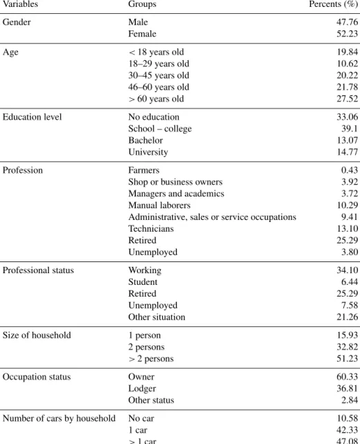
ac-Table 2. Description of the sociodemographic characteristics of the population in the case study area. Source: Insee (Census data, 2010, www.insee.fr).
Variables Groups Percents (%)
Gender Male 47.76
Female 52.23
Age <18 years old 19.84
18–29 years old 10.62
30–45 years old 20.22
46–60 years old 21.78
>60 years old 27.52
Education level No education 33.06
School – college 39.1
Bachelor 13.07
University 14.77
Profession Farmers 0.43
Shop or business owners 3.92
Managers and academics 3.72
Manual laborers 10.29
Administrative, sales or service occupations 9.41
Technicians 13.10
Retired 25.29
Unemployed 3.80
Professional status Working 34.10
Student 6.44
Retired 25.29
Unemployed 7.58
Other situation 21.26
Size of household 1 person 15.93
2 persons 32.82
>2 persons 51.23
Occupation status Owner 60.33
Lodger 36.81
Other status 2.84
Number of cars by household No car 10.58
1 car 42.33
>1 car 47.08
cumulation exceeded 600 mm in 12 h, causing 24 deaths and economic damages estimated at EUR 1.2 billion. A more de-tailed hydrometeorological description of this event is pro-vided in Delrieu et al. (2005). In terms of human impacts and death circumstances, more than half of the victims were outside buildings and five of them were vehicle-related fa-talities (Ruin et al., 2008). The flash flood event started on a Sunday evening, which might have limited the number of victims related to car driving accidents.
In order to evaluate daily mobility exposure to flash flood risk, the MobRISK output contains a record of the different road nodes crossed by the individuals on their route (includ-ing the road cuts), the time at which they passed these nodes and the individual exposure index (Eq. 1). The results are
presented in three main sections: (i) results of population mo-bility simulation, (ii) analysis of road submersion risk, and (iii) analysis of population exposure to road submersion.
4.2 Population mobility
The study area resident population is 111 511 individuals. An overview of the population sociodemographic characteristics is displayed in Table 2. As explained in Sect. 3.1, we used travel-activity data from the National Transport and Travel Survey to attribute programs of activities to the population in our study area. In order to respect the regional statistical rep-resentativeness of the survey sample and benefit from an ex-tensive schedule library with satisfactory variability, we se-lect travel-activity data corresponding to survey responders
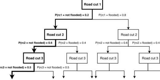
Figure 5. Probability tree diagram representing the method of measuring motorists’ flood risk exposure. The highlighted (bold lines) path
represents the example of a motorist who crossed 3 road cuts (rc) with the following probabilities of submersion: P (rc1=0.8), P (rc2=0.4)
and P (rc3=0.5). His/her exposure is represented as a probability tree diagram where the nodes are the encountered road cuts and the arcs
represent the probability of submersion in each road cut as shown in the Figure. First, we calculate the probability that the driver does not cross a flooded rod cut, which corresponds to the product of probability of no submersion in the crossed road cuts: P (not submerged road
cuts) = (1 − P (rc1)) ·(1 − P (rc2)) · (1 − P (rc3)) =0.06. Then, the final exposure corresponds to 1 − P (not submerged road cuts) = 0.94.
living in the Languedoc-Roussillon region (one of the 22 French Regions further divided into 5 “departments” includ-ing Gard). Since we are interested in motorists’ exposure, only individuals using principally motorized transport modes are selected: representing 1240 weekday schedules and 1087 weekend schedules.
We conducted a multi-factor discrepancy analysis on the different schedules in order to assess the effect of sociodemo-graphic variables on the activity sequence dissimilarities. We analyzed the effects of six variables: gender, age, education level, professional status, profession and household compo-sition. The choice of these variables is based on previous studies on the effect of sociodemographic characteristics on daily travel-activity behavior (Pas, 1984). These variables are considered the independent variables, and the matrix of
dis-similarities (dij)between sequences are the dependent
vari-ables. Similar to the ANOVA test, individuals are grouped based on the selected factors and we attempt to compare the inter-group and intra-group variance to measure how much the chosen factors explain the total variance. The variance is then calculated based on Eq. (2), where the sum of squares (SS) is expressed using the average pairwise squared dissim-ilarities (Anderson, 2001): SS = n X i=1 (yi− ¯y)2= 1 2n n X i=1 n X j =1 (yi−yj)2 = 1 n n X i=1 n X j =i+1 dij2. (2)
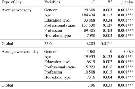
We observed that these selected variables explain 20 %
(R2=0.20) of the total discrepancy for the weekday
sched-ules and only 3 % (R2=0.03) for weekend schedules
(Ta-ble 3). Globally, there is a statistically significant effect of the selected variables on schedule discrepancy (p value < 0.05). For an average weekday, the most significant variable is the professional status (F = 157 530 and p < 0.05). For the weekend, results indicate that the majority of the variables provide moderate but significant contributions to explain the total discrepancy, except gender, which is not significant (F = 4060, p > 0.05).
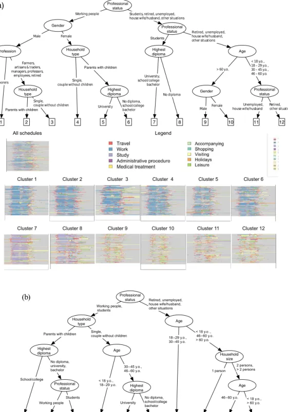
We displayed a regression tree analysis generating 12 clusters for weekday schedules representing three classes of working men schedules (clusters 1, 2 and 3), three classes of working women schedules (clusters 4, 5 and 6), two classes of students (clusters 7 and 8) and four classes of non-working persons depending on their age and gender (clusters 9, 10, 11 and 12; Fig. 6a). For weekend schedules, the regression tree generated 10 clusters composed of a class of students (clus-ter 3), five classes of working persons depending on their household type and age (clusters 1, 2, 4, 5 and 6), and four classes of non-working persons depending on their age and household size (clusters 7, 8, 9 and 10; Fig. 6b). These results are used to produce “if–then” rules for assigning 1 weekday schedules and 1 weekend schedules to the individuals living in the study area. Each individual, according to his sociode-mographic profile, is randomly assigned to one of the list of schedules corresponding to the appropriate cluster.
The MobRISK mobility model is implemented to simulate population mobility during 1 average weekend followed by an average weekday in order to simulate mobility patterns similar to the 8–9 September 2002 event, which happened to be a Sunday and a Monday. MobRISK generated in total 737 135 trips in total: 333 453 trips on Sunday and 403 682
Cluster 1 Cluster 2 Cluster 3 Cluster 4 Cluster 5 Cluster 6
Cluster 7 Cluster 8 Cluster 9 Cluster 10 Cluster 11 Cluster 12
All schedules Legend
(a) University No diploma school/college bachelor School/college No diploma, university, bachelor Single, couple without children
Working people Students 30– 45 y.o , 46– 60 y.o 18 – 29 y.o , 30 – 45 y.o Retired, unemployed, house wife/husband, other situations < 18 y.o , 18– 29 y.o < 18 y.o , 46– 60 y.o > 60 y.o 46 – 60 y.o 1 person 2 persons, > 2 persons < 18 y.o , > 60 y.o Working people, tudents (b) . . . . . . . . . . . . , s
Figure 6. Regression tree results for weekday schedules (a) and weekend schedules (b) indicating 12 and 10 clusters of schedules respec-tively. The upper part of the figure displays the regression tree: each node represents the variable splitting the schedules into two groups and each arc represents the group/category. A visual representation of the weekday schedules corresponding to each cluster is displayed at the bottom of (a) each activity, represented by a color, and each line, representing a sequence of activities.
Table 3. Results of the discrepancy analysis of activity sequences for each covariate in an average weekday and an average weekend. (SST)
is the sum of all schedule pairwise distances divided by the number of schedules; (SSW)is the sum of all schedule pairwise distances within
groups divided by the number of schedules; (R2)refers to the part of the discrepancy explained by the variables; (a) refers to the number of
groups in each variables; (N ) is equal to n(n − 1)/2, where n is the sample size. R2= SSB
SSt ;F =
SSB/(a−1)
SSW/(N −a). Formulas to calculate F and
R2for the total model are provided in Studer et al. (2011) and Anderson (2001).
Type of day Variables F R2 pvalue
Average weekday Gender 29 308 0.005 0.001***
Age 184 434 0.113 0.001*** Education level 33 868 0.034 0.001*** Professional status 157 530 0.127 0.001*** Profession 89 305 0.103 0.001*** Household type 7098 0.003 0.001*** Global 33.64 0.203 0.01**
Average weekend day Gender 4060 0 0.079
Age 19 935 0.153 0.001*** Education level 6819 0.007 0.001*** Professional status 15 923 0.016 0.001*** Profession 10 508 0.015 0.001*** Household type 7316 0.004 0.001*** Global 3.96 0.033 0.001***
* Significance level: p < 0.1; ** significance level: p < 0.05; *** significance level: p < 0.01.
Home Shopping Medical Administrative Visiting Accompanying Leisure Holidays Work Study
Travel goals P ercents 0 10 20 30 40 50 Sunday Monday
Figure 7. Distribution of simulated travel purposes between an av-erage Sunday and an avav-erage Monday. Over the Alès case study area, 737 135 trips were generated by the MobRISK model: 333 453 trips on Sunday and 403 682 on Monday.
on Monday. The average number of trips per individual was 3.06 on Sunday and 3.64 on Monday. When we examine the trip goals, we observe that more than 40 % of individuals’ trips are made to reach home. Obviously, the main difference between the weekdays and weekend in terms of trip goals is seen in the commuting trips, which are more important dur-ing weekdays, whereas visitdur-ing and leisure travels are more important during the weekend (Fig. 7).
4.3 Road network sensitivity to flooding
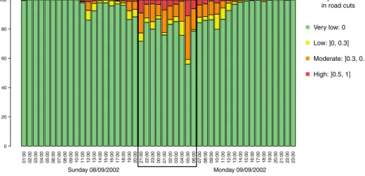
As mentioned in Sect. 3.2, a probability of submersion is assigned to every road cut by combining the flooding sus-ceptibility level of the road section and the return period of stream discharge in the river section. The CVN (Cevenne) distributed hydrological model (Vannier et al., 2016; Branger et al., 2010; Viallet et al., 2006) is used to compute the discharge at the 738 road cuts identified in the Alès case study in hourly time steps for the 2002 flash flood. The CVN model is especially developed for simulating hydrological re-sponses in flash flood events in the Cévennes region (south of France). Moreover, the implementation of the CVN model for reconstructing the 8 and 9 September 2002 event in the Gard region has provided satisfactory results (Braud et al., 2010; Anquetin et al., 2010). Discharge return periods are then computed at each road cut for hourly time steps and translated to submersion probabilities thanks to the relation-ship proposed by Naulin (2012, p. 93–94). Figure 8 shows that the period with the highest probability of road submer-sion takes place during the night of Sunday to Monday (8– 9 September), leading to “weak” population exposure since less people are on the roads in the middle of a Sunday night. The spatial distribution of the simulated road submersion hazard for the whole flash flood event period, computed by summing up the hourly probabilities of flooding, shows a concentration of high flooding hazard in the south of the Alès municipality.
01:00 02:00 03:00 04:00 05:00 06:00 07:00 08:00 09:00 10:00 11:00 12:00 13:00 14:00 15:00 16:00 17:00 18:00 19:00 20:00 21:00 22:00 23:00 00:00 01:00 02:00 03:00 04:00 05:00 06:00 07:00 08:00 09:00 10:00 11:00 12:00 13:00 14:00 15:00 16:00 17:00 18:00 19:00 20:00 21:00 22:00 23:00 P ercent of submersion r isk 0 20 40 60 80 100 Sunday 08/09/2002 Monday 09/09/2002 Probability of submersion in road cuts Very low: 0 Low: ]0, 0.3] Moderate: ]0.3, 0.5] High: ]0.5, 1]
Figure 8. Temporal distribution of the simulated probability of submersion at road cuts. Results obtained by the simulation of the MobRISK model for the 8–9 September 2002 flash flood event in the Alès study area (Gard).
4.4 Exposure analysis
A first method for assessing road users’ exposure to road flooding consists of quantifying the simulated traffic load in the potential road cuts identified in the study area during the 2 selected days. The computed exposure corresponds to the maximal exposure since the whole daily trips are assumed to be motorized. The results reveal that motorists were essen-tially exposed to road cuts corresponding to the two lowest levels of susceptibility (Table 4).
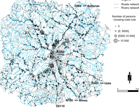
The spatial distribution of traffic load on potential road cuts shows a high motorist exposure on the main roads con-necting Alès to the other major cities of the area: road D6110, road N106, road D981 and road D904 (Fig. 9). Figure 10 shows the dynamics of road users’ exposure to potential road cuts represented by two peaks on Sunday, one at 10:00 lo-cal time (LT) and the other one at 16:00 LT, indicating, for the first peak, more than 25 000 motorists crossing potential road cuts per hour. On Monday 9 September, three peaks are detected at 07:00 LT, 13:00 LT, and 16:00 LT, correspond-ing to commutcorrespond-ing trips and reachcorrespond-ing 40 000 people crosscorrespond-ing potential road cuts per hour. The comparison between tem-poral dynamics of roads submersion probabilities and traffic load in potential road cuts indicates a clear lag time between the period corresponding to high road submersion probabili-ties and the one with a larger number of exposed road users (Fig. 11). Indeed, this lag time is considered an important factor contributing to reducing vehicle-related accidents and fatalities for the 2002 flash flood event in this area.
This exposure measurement provides an estimation of traf-fic load on potential road cuts. Hence, by combining the flood hazard, represented by the hourly probabilities of submer-sion at road cuts, with human exposure, given by maximal traffic load passing these road cuts, it is possible to iden-tify the number of persons who might have been endangered by crossing road cuts at the time they were submerged. The
proposed risk index (Eq. 3) characterizes the number of mo-torists who could be in effective danger by multiplying the probability of submersion in road cuts with the number of motorists crossing them for every hour time step.
N (Inddanger)rc,t=
Xnrc
i P (submersion)rc,t
·N (Indexposed)rc,t, (3)
where (rc) refers to the crossed road cut and (t ) is the time period.
In Fig. 11, the time evolution of the risk index reveals a different pattern from those associated with flooding haz-ard or with the traffic load at road cuts. The figure clearly illustrates that the period corresponding to the highest risk of flooding for road users occurred on 9 September from 05:00 LT to 11:00 LT with a peak at 07:00 LT, representing
more than 1500 motorists h−1in significant danger of
flood-ing. The spatial distribution of the risk index determined for the whole event shows that the majority of road cuts pre-senting a considerable danger in terms of potential victims are located around the Alès municipality (Fig. 12). The re-sults of the simulation for the entire event show that on aver-age 15 individuals might have crossed dangerous road cuts. Geolocated vehicle-related fatal accident data provided by Ruin et al. (2008) are used as a first evaluation of this re-sult. One vehicle-related victim (Fig. 12) was identified in our study area at a location that effectively corresponds to a road cut with high risk level (the 16th most dangerous road
cut, N (Inddanger) =162). The proposed risk index mapping
might thus provide an efficient indicator of flood risk magni-tude in the road network since it combines both environmen-tal and social parameters.
Finally, we investigate the effect of sociodemographic variables on individual exposure to road submersion. The MobRISK simulation of the probability, of each individual crossing submerged road sections on his daily route
indi-Alès D6110 N106 => Nîmes D981 => Uzès D904 => Aubenas Legend Roads network Rivers network Number of persons
crossing road cuts 0
]0, 5000] ]5000,10 000] > 10 000
0 10 km
Figure 9. Spatial distribution of simulated traffic load at road cuts during the flash flood event period. Results obtained by the simulation of the MobRISK model for the 8–9 September 2002 flash flood event in the Alès study area (Gard).
04:00 05:00 06:00 07:00 08:00 09:00 10:00 11:00 12:00 13:00 14:00 15:00 16:00 17:00 18:00 19:00 20:00 21:00 22:00 23:00 00:00 01:00 02:00 03:00 04:00 05:00 06:00 07:00 08:00 09:00 10:00 11:00 12:00 13:00 14:00 15:00 16:00 17:00 18:00 19:00 20:00 21:00 22:00 23:00 0 10 000 20 000 30 000 40 000 50 000 Number of e xposed persons Sunday 08/09/2002 Monday 09/09/2002
Figure 10. Temporal distribution of simulated traffic load at road cuts, which represent the hourly number of exposed persons. Results obtained by the simulation of the MobRISK model for the 8–9 September 2002 flash flood event in the Alès study area (Gard).
cates that the average individual exposure (Eq. 1) is 0.17 (a probability of 17 % of crossing submerged roads during the event period) with a variance of 0.10. A total of 75 % of the road users have a zero risk of crossing submerged road cuts. Individual exposure varies with sociodemographic characteristics such as age, gender, professional status and profession. For instance, men are more exposed than women
(Exposuremen=0.18; Exposurewomen=0.15). Not
surpris-ingly, workers are the most exposed, with an average risk of 0.28, while retired and unemployed individuals have an av-erage risk of 0.10. Managers, laborers and professors seem to be the most exposed professionals with an average ex-posure of 0.27 (Table 5). An analysis of variance (one-way ANOVA test) showed that the effects of the four selected variables are statistically significant (Table 6). The most ex-posed individuals are mainly young working males whose
Table 4. Maximal number of motorists crossing potential road cuts during the event period (individuals can be counted several times if they crossed many road cuts in their itineraries).
Sensitivity levels Number of Percent of road cuts Number of motorists Percent of motorists
of road cuts road cuts by sensitivity level (%) crossing road cuts (pers) crossing road cuts (%)
Very low 523 70.87 327 603 63.88 Low 103 13.96 81 488 15.89 Moderate 75 10.16 98 021 19.11 High 37 5.01 5742 1.12 Total 738 100 512 854 100 01:00 02:00 03:00 04:00 05:00 06:00 07:00 08:00 09:00 10:00 11:00 12:00 13:00 14:00 15:00 16:00 17:00 18:00 19:00 20:00 21:00 22:00 23:00 00:00 01:00 02:00 03:00 04:00 05:00 06:00 07:00 08:00 09:00 10:00 11:00 12:00 13:00 14:00 15:00 16:00 17:00 18:00 19:00 20:00 21:00 22:00 23:00 P ercent of submersion r isk 0 20 40 60 80 100 08/09/2002 09/09/2002 0 5000 10 000 15 000 20 000 25 000 30 000 35 000 40 000 45 000 Number of e xposed persons 0 500 1000 1500 2000
Number of persons potentially in danger
Probability of submersion in road cuts Very low: 0 Low: ]0, 0.3] Moderate: ]0.3, 0.5] High: ]0.5, 1] Exposed persons Persons potentially in danger
Figure 11. Time lag between the temporal distribution of the probability of submersion (colored bars) and the traffic load at road cuts (line). The dotted line represents the temporal distribution of the risk index referring to the number of persons potentially in danger (resulting from the combination of both the probabilities of submersion and traffic load). Results obtained by the simulation of the MobRISK model for the 8–9 September 2002 flash flood event in the Alès study area (Gard).
trips are generally more motorized and commute longer dis-tances daily (Debionne et al., 2016). These results confirm the benefit of integrating mobility behaviors into social vul-nerability assessment. This integration points out different socioeconomic vulnerability profiles that are usually not con-sidered when dealing with static (resident) vulnerability. The classic static social vulnerability index usually attributes a high vulnerability level to women, elders and persons with low professional status (Cutter et al., 2000). These social pro-files seem to be less exposed to road flash flooding.
5 Discussion and perspectives
The MobRISK microsimulator is to our knowledge the first of its kind in combining social and hydrometeorological state-of-the-art knowledge to understand the dynamics of hu-man exposure and behavioral response to short-fuse weather events. This first implementation of MobRISK shows the po-tential of this tool for emergency planning and road manage-ment in crisis situations. Other examples of microsimulations often use a multi-agent platform to simulate such dynamic in-teractions (see for instance, Dawson et al., 2011) nevertheless those models do not allow addressing the scale of a French
department (c.a. about 6000 km2) involving about 700 000
agents. Because MobRISK has just recently been developed, several improvements are planned for improving its reliabil-ity, optimizing its functioning and moving toward a more op-erational tool.
The next step of its development is to better reproduce the travel durations observed in the ENTD dataset. In fact, the activity-based mobility modeling approach requires data de-scribing the location of different activities conducted by the individuals. Whereas work and school activity locations are identified based on census data, it is more complicated to lo-cate secondary activities such as shopping and leisure activ-ities. We assume for this first application that secondary ac-tivities are located within a buffer of 500 m around the place of residency. However, future efforts are needed to improve the secondary activity location rules by taking into consider-ation travel costs and places knowledge (Marchal and Nagel, 2005). The buffer size used for secondary activity locations may affect the simulated travel durations. A comparison be-tween simulated trip duration in MobRISK and observed trip duration retrieved from the ENTD data indicates an under estimation of simulated travel durations, corresponding es-pecially to secondary activity travels (Fig. 13). This
underes-Alès D6110 N106 => Nîmes D981 => Uzès D904 => Aubenas Legend Roads network Rivers network Number of persons potentially in danger 0 ]0, 15] ]15,100] > 100 0 10 km Location of the vehicle-related victim
Figure 12. Spatial distribution of the risk index computed with the MobRISK simulator for the 8–9 September 2002 flash flood event in the Alès study area (Gard). It represents the potential number of endangered motorists who crossed flooded roads during the event period. The location of the past victim (black square) corresponds to a road cut with a high risk index.
Table 5. Motorists’ exposure mean and standard deviation per sociodemographic characteristics. The bold numbers refer to the most exposed groups by variable.
Variables Groups Exposure Exposure
(mean) (standard deviation)
Gender Male 0.18 0.31
Female 0.15 0.34
Age <18 years old 0.14 0.30
18–29 years old 0.21 0.36
30–45 years old 0.23 0.37
46–60 years old 0.20 0.35
>60 years old 0.11 0.26
Profession Farmers 0.16 0.32
Shop or business owners 0.21 0.36
Managers and academics 0.28 0.40
Manual laborers 0.27 0.39
Administrative, sales or service occupations 0.27 0.39
Technicians 0.22 0.36
Retired 0.10 0.25
Unemployed 0.13 0.29
Professional status Working 0.28 0.39
Student 0.22 0.36
Retired 0.10 0.25
Unemployed 0.10 0.26
House wife/husband 0.09 0.25
Commuting travel duration (weekday) Travel duration (mn) Frequency (%) 1 10 100 0 10 20 30 40 50 60 70 80 90 100 MobRISK simulations ENTD data
Commuting travel duration (weekend)
Travel duration (mn) Frequency (%) 1 10 100 0 10 20 30 40 50 60 70 80 90 100 MobRISK simulations ENTD data
Secondary activities travel duration (weekday)
Travel duration (mn) Frequency (%) 1 10 100 0 10 20 30 40 50 60 70 80 90 100 MobRISK simulations ENTD data
Secondary activities travel duration (weekend)
Travel duration (mn) Frequency (%) 1 10 100 0 10 20 30 40 50 60 70 80 90 100 MobRISK simulations ENTD data
Figure 13. Comparison of travel duration distributions obtained from the MobRISK simulations and ENTD data for a weekday and a weekend and corresponding to commuting and secondary activity trips (we presented only trips with duration less than 60 min, which represents more than 94 % of all the trips).
Table 6. Results of analysis of variance (ANOVA) for testing the effect of sociodemographic variables on individual submersion risk. Formulas to calculate the F and p value are provided in Anderson (2001). Variables pvalue Gender F (1, 32 637) = 48.03 0.00*** Age F (4, 32 634) = 166.5 0.00*** Professional status F (5, 32 633) = 366.9 0.00*** Profession F (7, 32 631) = 174.6 0.00***
* Significance level: p < 0.1; ** significance level: p < 0.05; *** significance level: p < 0.01.
timation may be explained by the buffer size selected for sec-ondary activity location, which seems to be too small com-pared to the real size of activities’ space and the shortest path criteria used for route choice. As a consequence, our model currently underestimates the computed motorist exposure.
Another important issue is the investigation of the link be-tween exposure and human impact. The individual exposure measurement is merely defined as the probability of encoun-tering flooded roads without taking into account the water height and flow level. This limitation is due to the difficulty in providing the necessary information because of the large number of parameters that need to be integrated regarding road infrastructures and geomorphologic specificities of road cuts. On the social side, understanding behavioral responses is key to the estimation of human impacts. Recently, this as-pect has been taken into account in MobRISK, which now incorporates a decision-making module to consider possi-ble activity rescheduling decisions and mobility adaptation to weather disruptions. The integration of individual deci-sions and coping capacities enables us to shift from expo-sure meaexpo-surement to social vulnerability quantification (Terti et al., 2015). To advance in this direction, the use of well-described, geolocalized, time-stamped and reliable human