HAL Id: dumas-02011699
https://dumas.ccsd.cnrs.fr/dumas-02011699
Submitted on 8 Feb 2019
HAL is a multi-disciplinary open access archive for the deposit and dissemination of sci-entific research documents, whether they are pub-lished or not. The documents may come from teaching and research institutions in France or abroad, or from public or private research centers.
L’archive ouverte pluridisciplinaire HAL, est destinée au dépôt et à la diffusion de documents scientifiques de niveau recherche, publiés ou non, émanant des établissements d’enseignement et de recherche français ou étrangers, des laboratoires publics ou privés.
submersions of roads due to flash floods in the Gard
region
Kim Thanh Nguyen
To cite this version:
Kim Thanh Nguyen. Spatio-temporal analysis of the exposure of motorists to submersions of roads due to flash floods in the Gard region. Life Sciences [q-bio]. 2018. �dumas-02011699�
Analyse spatio-temporelle de l'exposition des
automobilistes aux submersions des routes dues
aux crues rapides dans le département du Gard
Par : Kim Thanh NGUYEN
Soutenu à Rennes le 27/06/2018 Devant le jury composé de :
Hervé Nicolas Samuel Corgne
Maître de stage : Isabelle Ruin
Les analyses et les conclusions de ce travail d'étudiant n'engagent que la responsabilité de son auteur et non celle d’AGROCAMPUS OUEST
Ce document est soumis aux conditions d’utilisation
«Paternité-Pas d'Utilisation Commerciale-Pas de Modification 4.0 France» disponible en ligne http://creativecommons.org/licenses/by-nc-nd/4.0/deed.fr AGROCAMPUS OUEST CFR Angers CFR Rennes Année universitaire : 2017 - 2018 Spécialité : TELENVI
Spécialisation (et option éventuelle) : ………
Mémoire de fin d’études
d’Ingénieur de l’Institut Supérieur des Sciences agronomiques, agroalimentaires, horticoles et du paysage
de Master de l’Institut Supérieur des Sciences agronomiques, agroalimentaires, horticoles et du paysage
Fiche de confidentialité et de diffusion du mémoire
Confidentialité
Non Oui si oui : 1 an 5 ans 10 ans
Pendant toute la durée de confidentialité, aucune diffusion du mémoire n’est possible (1). Date et signature du maître de stage (2) :
(ou de l’étudiant-entrepreneur)
A la fin de la période de confidentialité, sa diffusion est soumise aux règles ci-dessous
(droits d’auteur et autorisation de diffusion par l’enseignant à renseigner).
Droits d’auteur
L’auteur(3) Nom Prénom -NGUYEN Kim Thanh-
autorise la diffusion de son travail (immédiatement ou à la fin de la période de confidentialité)
Oui Non
Si oui, il autorise
la diffusion papier du mémoire uniquement(4)
la diffusion papier du mémoire et la diffusion électronique du résumé
la diffusion papier et électronique du mémoire (joindre dans ce cas la fiche de conformité du mémoire numérique et le contrat de diffusion)
accepte de placer son mémoire sous licence Creative commons CC-By-Nc-Nd (voir Guide du mémoire Chap 1.4 page 6)
Date et signature de l’auteur :
Autorisation de diffusion par le responsable de spécialisation ou son
représentant
L’enseignant juge le mémoire de qualité suffisante pour être diffusé (immédiatement ou à la fin de la période de confidentialité)
Oui Non
Si non, seul le titre du mémoire apparaîtra dans les bases de données. Si oui, il autorise
la diffusion papier du mémoire uniquement(4)
la diffusion papier du mémoire et la diffusion électronique du résumé la diffusion papier et électronique du mémoire
Date et signature de l’enseignant :
(1) L’administration, les enseignants et les différents services de documentation d’AGROCAMPUS OUEST s’engagent à respecter cette confidentialité.
(2) Signature et cachet de l’organisme
(3).Auteur = étudiant qui réalise son mémoire de fin d’études
(4) La référence bibliographique (= Nom de l’auteur, titre du mémoire, année de soutenance, diplôme, spécialité et spécialisation/Option)) sera signalée dans les bases de données documentaires sans le résumé
Résumé
Les crues rapides sont considérées comme l'une des catastrophes naturelles les plus meurtrières en raison de leur courte échelle temporelle qui laisse peu de temps aux personnes exposées pour réagir. Des études récentes ont montré qu’un peu près de la moitié des victimes sont liées au véhicule et que la mobilité quotidienne devient un facteur important qui affecte l'exposition sociale aux crues rapides.
Ce rapport présente le travail du stage de fin d’études de NGUYEN Kim Thanh. Le rapport est présenté dans 5 parties principales:
Etat de l’art et positionnement de recherche
La partie 2 aborde les facteurs pouvant affecter les décisions d'adaptation de chaque individu : les facteurs contextuels (intensité des précipitations, niveau de submersion de la route, visibilité, alertes informations, etc.) et les facteurs cognitifs (évaluation du danger ou évaluation de l'importance de la flexibilité du motif de déplacement de chaque individu, etc.).
Cette partie présente également des résultats de la mise en œuvre du modèle de prise de décision dans MobRISK - un modèle de mobilité activité-centré utilisé pour simuler l'exposition des automobilistes dans les crues rapides en intégrant les comportements d'adaptation de la mobilité aux perturbations environnementales dans la thèse de Shaif Shabou.
Donc l’objectif du stage est basé sur les résultats précédents: la compréhension et la calibration du modèle MobRISK
Tester l'influence de différents facteurs sur l'exposition individuelle (évaluation de la flexibilité du motif du voyage, effet de l’âge et du sexe des individus en ce qui concerne leurs attitudes face aux risques, les conditions de la visibilité, niveau de la confiance dans les informations d’alerte)
Cas d’étude
La première application du MobRISK modèle est réalisée pour évaluer l’exposition des automobilistes aux submersions des routes dans la région d'Alès dans le département du Gard dans le sud de la France lors d’une crue éclair du 8 au 9 septembre 2002.
Cette partie présente des caractéristiques naturelles et sociales du département du Gard ainsi que l’évènement de crue rapide le 8-9 Septembre 2002. Cet évènement est considère comme l’un des évènements hydrométéorologiques les plus importants de la région et a 23 blessés.
La zone d’étude sélectionnée dans le Gard département comprends 61 communes situées autour la commune d’Alès. Une victime a été enregistrée dans cette zone d’étude.
MASTER 2 TELENVI
Données et méthodes
La partie 3 décrit les données d'entrée du modèle MobRISK: données géographiques et données sociales. Ils sont stockés et connectés dans une base de données. Les données géographiques contiennent les informations spatiales des réseaux fluviaux et routiers, la probabilité de submersion aux coupures de routes, les niveaux de précipitations, etc. Alors que les données sociales contiennent des informations sur les caractéristiques sociodémographiques des individus et leur mobilité (leurs emplois du temps).
Cette partie décrit également les 3 composants principaux du modèle (module de simulation des mobilités, des changements environnementaux et des décisions d’adaptation), ainsi que les méthodes utilisées pour créer le modèle des décisions et la méthode pour tester l'influence de facteurs différents sur l'exposition individuelle (changer les paramètres pour évaluer leurs effets de ces facteurs sur l'exposition des automobilistes).
Résultats et discussion
La partie 4 présente les étapes du travail du stage par un schéma de calcul. Il y a deux étapes principales : la première étape consiste à lancer les simulations des scenarios différents dans MobRISK, la deuxième étape consiste à utiliser les résultats de sortie de MobRISK pour analyser l'exposition de la population.
Les résultats du lancement de différentes simulations pour les scénarios différents montrent qu'il existe une variabilité importante entre chaque simulation et entre chaque exposition individuelle et que les changements de paramètres dans le modèle de décision n'ont pas vraiment affecté le résultat final. Les travaux futurs devront continuer à comprendre et expliquer les résultats des simulations du modèle et étudier des façons différentes de réduire la variabilité de l'exposition entre différentes simulations.
Acknowledgments
I would like to express my very great appreciation to Dr. Isabelle Ruin, my supervisor of my internship who have patiently guided me throughout 5 months of my internship with enthusiastic encouragement. I would also like to thank all my colleagues from the laboratory IGE, especially the members of HMCIS team.
My special thanks are extended to the members of Master 2 TELENVI 2017-2018, two dedicate supervisors Hervé Nicolas and Samuel Corgne and my fellow colleagues, especially Valentine Aubard, Laurène Torterat and Ou Jie who have supported me throughout my master.
Finally, I wish to thank my Vietnamese friends at home, in Grenoble and of course my family for their support and encouragement throughout my study.
MASTER 2 TELENVI GLOSSARY ENTD IGE IGN IFSTTAR INDCVI INSEE LTHE OHMCV RFL
Enquêtes Nationales Transports et Déplacements Institut des Géosciences de l’Environnement
Institut national de l'information géographique et forestière
Institut français des sciences et technologies des transports, de l'aménagement et des réseaux
Individus localisés au canton-ville
Institut National de la Statistique et des Etudes Economiques Laboratoire d’étude des Transferts en Hydrologie et Environnement Observatoire Hydrométérologique Méditerranéen Cévennes-Vivarais Revenus Fiscaux Localisés
Table of materials
1. Introduction ... 1
2. State of the art and research positioning ... 1
3. Case study ... 3
4. Data and methods ... 4
4.1. Input data ... 4
4.2. How the MobRISK model works? ... 6
5. Results and discussion ... 10
5.1. Calculation scheme ... 11
5.2. Results of simulations and discussion ... 13
6. Conclusion ... 19
List of figures ... 20
List of tables ... 21
References ... 22
1. Introduction
Flash floods are among the world’s most dangerous natural disasters, according to World Meteorological Organization, flash floods are the cause for more than 5000 lives lost annually with many damages to property. There are many definitions of flash floods, however, Montz and Gruntfest (2002) has distinguished several characteristics of flash floods that are generally agreed like: sudden, fast, violent, rare, occurring in small spatial scale and associated with other events such as storms, riverine floods or mudslides. Because of the notably short temporal scales of flash floods, forecasting flash flooding is still a challenge.
Many studies have shown that the circumstances in which flood fatalities most often occurred are vehicle-related (Ruin et al., 2008; Jonkman and Kelman, 2005; Terti et al., 2017). However, the development of a tool to estimate the social exposure to these hydro-meteological events, more particularly the exposure of motorists who represent a large part of the victims is still limited.
In terms of flash flooding modeling, many hydro-meteorological models have been developed. These models help to represent and simulate physical processes to understand and predict the dynamics of the natural hazard. On the other hand, these physical processes need to be combined with the daily mobility of people in order to assess their exposure to such short-fuse event. Modeling mobility behaviors has been a goal for the planning and management of transport demand to simulate daily trips at individual level.
A model called MobRISK has been developing at LTHE as part of the MobiClimEx project to meet the needs of coupling physical and social dynamics. MobRISK is an activity-based mobility model which is specifically used to simulate motorists’ exposure in flash flood events by integrating mobility adaptation behaviors with environmental perturbations. The model has 3 versions. In the first version (version 1.0), a database was created to connect the sociodemographic characteristics of the population, their daily mobility with the geographic data. In the second version (version 2.0), the temporalities of displacements and road submersions were added. Finally, the third version (version 2.1) integrated the adaptation of the mobility behaviors by developing a decision-making model in the case of environmental perturbations. The MobRISK model mentioned hereafter is the final version with the decision model implemented.
This report presents the work has been done in the internship effectuated at IGE, which is the merge of 2 laboratories, one of them is LTHE. This internship continues the work of the PhD thesis of Saif Shabou.
2. State of the art and research positioning
Concerning the behaviors of individuals when facing situation of flash flooding, there are two main types of factors that can affect the decisions of adaptation: contextual factors and cognitive factors. The contextual factors are the information that can be observed or received by the individuals such as intensity of precipitation, road submersion level, visibility (day / night), reactions of people around; damages of roads, cars…; alerts information. The cognitive factors are related to the internal perception of each individual such as the
2 evaluation of threat and danger; or the evaluation of the importance of flexibility of the travel motive. The evaluation of danger can depend on not only the contextual factors but also the sociodemographic characteristics (age, sex, etc…) of the individuals (Mileti, 1995; Ruin, 2007).
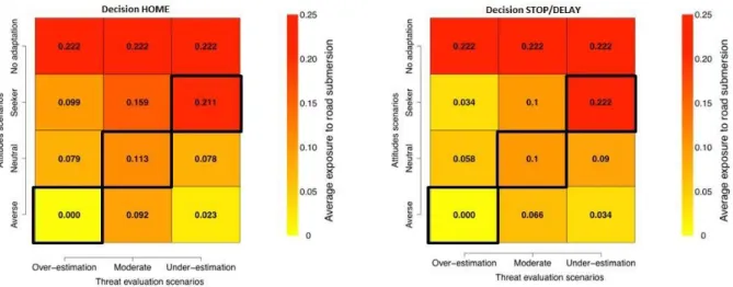
Shabou (2016) in his PhD thesis has implemented the decision-making model into the MobRISK model in order to evaluate the effect of different levels of evaluation of danger and different attitudes to risks on motorists’ exposure. By testing different scenarios with four levels of attitudes to risk (“No adaptation”, “Risk seeker”, “Risk neutral” and “Risk averse”), three levels of evaluation of danger (“High risk perception”, “Moderate risk perception” and “Low risk perception”) and two types of decisions “HOME” (return home) or “STOP/DELAY” (stop or delay the next activity), he finds that the adoption of "risk averse” attitude reduces the average exposure of motorists by half and divides the percentage of people exposed by three; over-estimation of danger (high risk perception) reduces drivers’ exposure by half compared to a moderate estimate; the adoption of an attitude of risk aversion with an over-estimation of the danger makes it possible to completely cancel the exposure of the motorists. Concerning the effect of the types of decision, Shabou (2016) finds that decisions to stop (an hour) or wait (30 minutes) in front of a submerged road or to shift travel by re-planning daily activities (STOP/DELAY) reduce the average exposure of motorists more than returning to the place of residence (HOME). Figure 1 shows the results of Shabou (2016)
Figure 1:Results of implementation of the decision-making component into MobRISK
(Shabou, 2016)
The main objective of the internship is then understanding and exploiting the potentialities of the MobRISK model, especially the decision-making model to evaluate the effects of different factors on the motorists’ exposure to road submersion in flash floods events.
The first factors is the evaluation of the flexibility of the travel’s motive, which is one of three main components that can play a significant role in the mobility adaptation’s decisions (Cools and Creemers, 2013; Ruin, 2007; Terti et al., 2015), alongside with the evaluation of the effect of different levels of evaluation of danger and different attitudes to
MASTER 2 TELENVI
3 risks which have been tested in the PhD thesis of Shabou (2016). If the activity has strong flexibility, it means that the activity is more easily modified or canceled. The study of Shabou (2016) has defined the flexibility of activities according to Cools and Creemers (2013) and Ruin et al. (2014), which means that people more easily cancel trips related to leisure or shopping than trips to work and study. Thus, it would be interesting to see how the exposure of the population change if all the types of activities are considered flexible or not flexible.
The second factor is taking into account the effect of age and sex of individuals with respect to their attitudes toward risks. According to Jonkman and Kelman (2005) and Coates (1999), age and sex are discriminating factors in increasing the vulnerability and exposure of individuals to flash floods in mobility situations. Many studies have shown that the majority of the victims are the male motorists and younger than 60 years old (Terti et al, 2017; Ruin et al., 2008; Abramovich et al., 1995).
The third factor is the visibility conditions which affects the driving conditions and has a significant effect on travel choices (Kilpeläïnen and Summala, 2007). In the thesis of Shabou (2016), he considered that visibility depends on rainfall level and luminosity (day or night) so it would be interesting to take into account the time of dusk and dawn which has also proved to be a risk factor for drivers in flash flood conditions (Terti et al., 2017).
The fourth factor to be evaluated is the level of trust in alert information. In fact, the level of trust affects the level of risk perception so it definitely affects the decision of the drivers in the case of flash floods (Mileti, 1995).
3. Case study
The MobRISK model was designed to estimate the exposure of population in the Gard department, in the Languedoc-Roussillon region now part of the new Occitanie in southeastern France. According to INSEE’s data, there were 736 029 inhabitants living in 5853 km2 surface of the Gard department in 2014. The most populated municipalities are Nȋmes and Alès with 154,349 and 41,249 inhabitants respectively.
The region has a typical Mediterranean climate characterized by frequent and very strong storms that occur mostly in autumn (Delrieu et al., 2005, Gaume et al., 2009). On the other hand, the southeastern half of the region consisted of calcareous plateaus at altitudes ranging from 50 to 300 m above sea level, while the northwestern half is mountainous with various bedrocks and reaches 1700 m ASL at its highest points (Versini & al., 2010). These characteristics often create flash floods which are violent and deadly in this region. Since the middle of the 13th century until 2013, Gard has experienced more than 500 recorded floods1. From 1316 to 1999, Antoine et al., (2001) censed 27 fatal flood episodes which caused 277 deaths in the Gard area.
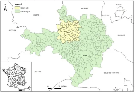
The first application of the MobRISK model is to evaluate the exposure of motorists to road submersions that are due to the major flash flood event of 8-9 September 2002 in a study area of the northwest Gard department. The selected study area within the Gard consists of 61 municipalities located around Alès (Figure 2). The study area includes 111,511 residents.
4
1
http://www.noe.gard.fr
Figure 2: Map of the study area around Alès
The event on September 8th and 9th, 2002 is considered one of the most important hydro-meteorological events in the region. It caused 23 casualties and the economic damage estimated is 1.2 billion euros. The study of Ruin et al. (2008) shows that among 23 victims, 13 of them occurred outside (5 motorists trapped in their vehicles, 5 people camping and 3 people walking) and the other 10 victims lost their lives in their homes. The only victim recorded in the study area was a motorist located in St Christol les Ales (the commune south of Alès).
4. Data and methods 4.1. Input data
The input data required in the MobRISK model consists of both geographical and social data; they are stocked and connected in a database by using SpatiaLite, the spatial extention of SQLiTe (a library written in C language that proposes a relational database engine accessible by the SQL language).
The geographical data contains the spatial information of the river and road networks, probability of submersion at road cuts, precipitation levels, locations of activities, etc... Table 1 provides a short description and sources of the data. Concerning the data of activities’ areas, the data from RFL which contains information about the number of households or individuals and their sociodemographic description is provided at 200 m x 200m resolution; the work and school activities’ data are generated by assigning a road node inside a buffer with a radius of 200 m around the administrative centers of work and school municipalities, provided by MOBPRO (professional mobility) and MOBSCO (school mobility) datasets; and a road node inside a buffer of 500 m around the administrative center of each individual’s residence is randomly assigned for other activities’ location (shopping, leisure,…).
MASTER 2 TELENVI
5
Table 1:Geographical input data of MobRISK
Data Description Sources
Administrative units Administrative boundaries BD GEOFLA Activities’ areas Location of the various activities’ zones:
- Household: RFL: tiles/squares de 200m
- Work/Study: MOBPRO and MOBSCO: buffer of 200 m around the administrative centers.
- Other (leisure, shopping, etc...): buffer of 500m around their place of residence.
INSEE
Hydrographic network Hydrographic network: 6 large watersheds BD
CARTHAGE Road network Road sections that are characterized by various attributes: the
vocation (informs the importance of the section for road traffic), the number of lanes, the administrative class (motorway, national road or departmental road) ...
BD CARTO - IGN
Road cuts (Versini et al., 2010; Naulin et al., 2012)
Identification of the different road-river intersections sensitive to flooding, their sensitivity levels (very low/ low/ moderate/ high), and the range of discharge’s return periods for which there are susceptible to be submerged.
IFSTTAR
Precipitation Rainfall levels recorded during past events OHMCV Road submersion Simulation of the dynamic of submersion probabilities at road cuts
based on the CVN distributed hydrological model outputs for past events (2002, 2005, 2008)
LTHE/IGE
Concerning the road cuts (road sections susceptible to flooding) dataset, Versini et al. (2010) carried out a discriminant analysis of the geomorphological characteristics of an inventory of road flooding during the last 40 years according to three main factors: the attitude, the local slope and the drained area. 1970 road cuts are then classified into 4 sensibility levels to flooding: very low s0 (1093 points) which has the return period of
flooding more than 40 years, weak s1 (359 points), medium s2 (297 points) and high s3 (221
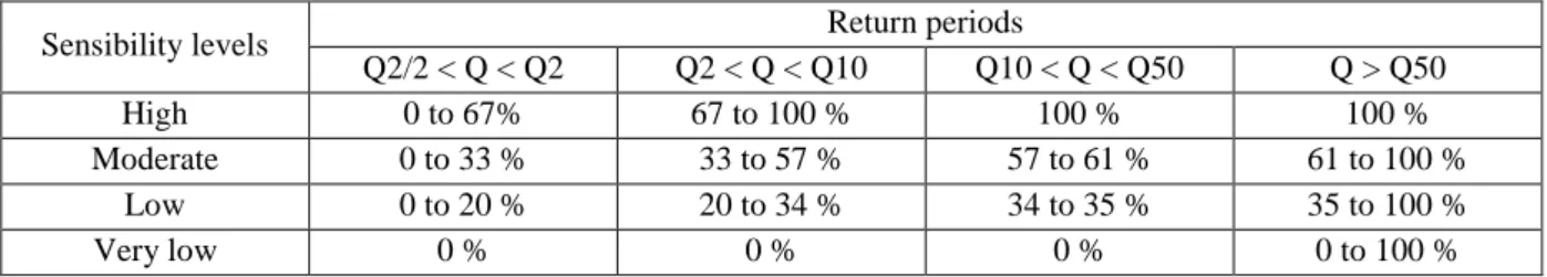
points) have the empirical return period smaller than 1 year in 20, 35 and 65 % of the points respectively. Naulin (2012) analyzed the probability of submersion for each road cut by combining the sensibility classes, defined by Versini et al. (2010), with the simulated peak flows (using a rain-flow hydrological model) at the river sections containing these road cuts (Table 2). For the case of the September 2002 flash flood event in the Gard, The CVN distributed hydrological model developed at LTHE (Vannier et al., 2016) was run for each sensitive road cuts of the study area to define the chronology of the probability of submersion.
6
Table 2: Probability of submersion associated with different sensibility classes according to
the return period of peak flow (Naulin et al., 2012)
Sensibility levels Return periods
Q2/2 < Q < Q2 Q2 < Q < Q10 Q10 < Q < Q50 Q > Q50 High 0 to 67% 67 to 100 % 100 % 100 % Moderate 0 to 33 % 33 to 57 % 57 to 61 % 61 to 100 %
Low 0 to 20 % 20 to 34 % 34 to 35 % 35 to 100 %
Very low 0 % 0 % 0 % 0 to 100 %
On the other hand, the description of the social data which is used in MobRISK is shown in Table 3. The social data contains information about the sociodemographic characteristics of individuals and their mobility (daily schedules). The former is the combination of INDCVI, MOBPRO and MOBSCO datasets while the latter is based on ENTD data. 10 categories of travel reasons are proposed: home, school, working, shopping, medical appointment, administrative procedure, visiting, accompanying, leisure and holiday activities.
Table 3: Social input data of MobRISK
Data Description Sources Details
Census (Rp)
Socio-demographic
characteristics of individuals and households
INSEE Sex, age, highest degree, professional situation, profession, number of persons in household, number of children, mode of transport…
Mobility (ENTD)
Mobility of the population INSEE Description of sociodemographic characteristics of individuals and their households (profession, age, sex, number of persons…)
Description of their mobility on 1 weekday and 1 weekend (number of trips, mode of transport, trips’ purposes, time of departure and arrival)
4.2. How the MobRISK model works?
The MobRISK model includes 3 principal components: (i) an activity-based mobility
model generates individual road trips; (ii) an environmental changes model simulates different
changes of environment such as road submersions, precipitation levels … and (iii) a
decision-making model predicts individual decisions according to different scenarios. The first two
components are created in the C++ programming language and the last one is coded in LUA language.
The different simulations are managed by a Discrete Event Simulator (DES) - a computer modeling technique that represents the state changes of a given system as a series of discrete events.
MASTER 2 TELENVI
7
Figure 3: Architecture of MobRISK (Shabou, 2016)
The MobRISK model use the activity-based approach, an approach that incorporate behavioral and psychological components and decision-making processes (Shabou et al., 2017) for mobility modeling. From the mobility data (ENTD) that is mentioned in the previous section, Shabou et al (2017) measured the level of similarity between sociodemographic variables (gender, age, education level, professional status) and the sequences of activities by using the discrepancy analysis method proposed by Studer et al. (2011). Based on the results of the dissimilarity analysis, Shabou et al. (2017) produced a classification of the activity sequences according to the socio-demographic variables by using the regression tree analysis method also proposed by Studer et al. (2011). This means that the activity sequences that have more similarities in their sociodemographic characteristics would be put in to the same classification.Each individual of the population is then connected to an average weekend schedule (to simulate the Sunday September 8, 2002) and an average weekday schedule (to simulate the Monday September 9, 2002).
The MobRISK model considers four kinds of events in its simulations. These events are moments when there is a change in the state of the system and the decision-making model is implemented:
- Bottleneck: the individual meets one of a possible submerged road section (road cuts). - Activity-end: the end of the current activity and change of the travel purpose of the
individual.
- Environmental cue: the individual’s perception of a sign of changes in environmental or weather conditions.
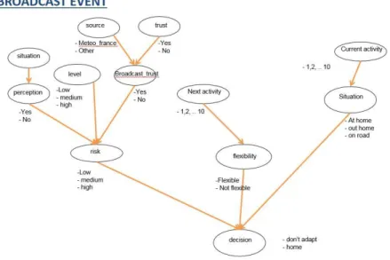
- Broadcast: the individual receives alert information.
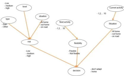
The decision-making modeling is based on Bayesian networks (Belief Networks) or probabilistic graphical models – allowing to visualize the dependencies (and independences) between the variables used and also provide an intuitive visual tool of representation (Shabou, 2016).
8 The basic equations of Bayesian networks are presented below:
( | ) ( ) ( )
where: ( | ) is the probability of event X knowing the observation of event Y; ( ) is the probability of the intersection of events X and Y (realization of X and Y);
( ) is the prior probability of event Y.
The equation to calculate the probabilities joined on all the variables is: ( ) ∏ ( | ( ))
The Bayesian networks of 4 events (Bottleneck, Activity end, Environment cue and Broadcast) that were built are shown in Figure 4, 5, 6 and 7.
Figure 4: Bayesian network of Bottleneck event (Shabou, 2016)
MASTER 2 TELENVI
9
Figure 6: Bayesian network of Environment cue event (Shabou, 2016)
Figure 7: Bayesian network of End of activity event (Shabou, 2016)
The creation of the decision-making model consists of not only defining the variables and their relations in the Bayesian network but also defining the parameters of the model which are represented in the conditional probability tables. All the conditional probability tables are presented in Annexes.
Once the simulation of MobRISK model is started, the environmental cues events and broadcast events are imported and placed on the time axis (called "scheduler"). Then, for each individual, the first activity planned in the schedule is recorded. At the end of the first activity (activity-end event), if MobRISK identifies that the individual decides to continue his/her plan, MobRISK identifies the place of the next activity and use the Dijkstra algorithm to calculate the shortest route in time to reach the location by moving the individual on the nodes of the road network. The model records the arrival times at each road node. If one of these nodes corresponds to a road cut point, the decision-making model is implemented to identify the decision of the individual in relation to the next activity (Bottleneck events). This procedure is repeated for all individuals until the end of the simulated flash flood event period.
10 The motorists’ exposure to road submersion is finally calculated from the probability of submersion at road cuts that can be encounter by individuals according to their itineraries:
( ) ∏ ( ( ))
where: ( ) is the individual’s exposure
( ) is the probability of submersion at the kth
road cuts crossed by individual.
For example, if the individual meets three road cuts on his/her routes with the probability of submersion at each road cut is 0,3; 0,7 and 0,2 respectively. Then his/her exposure to road flooding is calculated as:
E(ind) = 1 – [(1 – 0,3)*(1 – 0,7)*(1 – 0,2)] = 0,832
5. Results and discussion
In order to better understand the Bayesian networks, an example of the calculation from the values of the conditional probabilities of all the parameters to the probability of the decisions. Supposing we are in the “bottleneck” event and the scenario of attitude to risk is “risk averse”, the Bayesian network of this event is presented in Figure 4 and the tables of conditional probabilities are in Annexes.
We suppose that luminosity = “day”, rain = “high”, the probabilities of level of visibility can be found in the table of conditional probabilities are:
P(visibility = “good” | luminosity = “day”, rain = “high”) = 0.3 P(visibility = “bad” | luminosity = “day”, rain = “high”) = 0.7
If the submersion = “high”, then:
P(risk = “low”)
= P(risk = “low” ∩ visibility = “good” ∩ submersion = “high”) + P(risk = “low” ∩ visibility = “bad” ∩ submersion = “high”)
= P(risk = “low” | visibility = “good”, submersion = “high”) x P(visibility = “good”) + P(risk = “low” | visibility = “bad”, submersion = “high”) x P(visibility = “bad”)
= 1 x 0.3 + 1 x 0.7 = 1
We also suppose that the individual is in an activity of type = “study”, so:
P(flexibility = “flexible” | activity = “medical”) = 0.4 P(flexibility = “not flexible” | activity = “medical”) = 0.6
The probability of decision knowing level of risk, flexibility and attitude according to the conditional probability table:
P(decision = “keep planned” | risk = “low”, flexibility = “flexible”, attitude = “risk averse”) = 0.5
P(decision = “stop” | risk = “low”, flexibility = “not flexible”, attitude = “risk averse”) = 0.5
MASTER 2 TELENVI
11
= P(D = “keep planned” ∩ R = “low” ∩ F = “flexible” ∩ A = “risk averse”) + P(D = “keep planned” ∩ R = “low” ∩ F = “not flexible” ∩ A = “risk averse”)
= (P(D = “keep planned”| R = “low” ∩ F = “flexible” ∩ A = “risk averse”) x P(R = “low” ∩ F = “flexible” ∩ A = “risk averse”)) + (P(D = “keep planned”| R = “low” ∩ F = “not flexible” ∩ A = “risk averse”) x P(R = “low” ∩ F = “not flexible” ∩ A = “risk averse”))
= (P(D = “keep planned”| R = “low” ∩ F = “flexible” ∩ A = “risk averse”) x P(R = “low”) x P(F = “flexible”) x P(A = “risk averse”)) + (P(D = “keep planned”| R = “low” ∩ F = “not flexible” ∩ A = “risk averse”) x P(R = “low”) x P(F = “not flexible”) x P(A = “risk averse”))
= (0.5 x 1 x 0.4 x 1) + (0.5 x 1 x 0.6 x 1) = 0.5
P(D= “stop”) = 1 - 0.5 = 0.5
The previous sections describe the comprehension of the model MobRISK, its input data, its methods and the results of the premier application in the Gard region during the flash flood event on 8-9 September 2002. Based on the understanding of the model and its codes (in R and LUA programming language), the next section will present the results obtained from testing different new scenarios, which involving changes in four factors mentioned in section 2 (flexibility of travel’s motive, the risk attitude related to age and sex, visibility and trust in broadcasts).
5.1. Calculation scheme
The first step is running the simulations in MobRISK. In order to run the model’s simulations; we have to define the database (test.traffix) and the decision-making model (scripts LUA). 20 simulations are run for each scenario. Shabou (2016) have 4 levels of attitude to risk (“risk averse”, “risk neutral”, “risk seeker” and “no adaptation”). Each type of attitude is associated with a conditional probability table where the chances of taking the decision KEEP PLANNED and HOME or KEEP PLANNED and STOP/DELAY vary (see an example in Annex p.28). For instance, if the scenario is “risk averse”, there are more people to return home or stop-and-wait than in the scenario “risk seeker”. We decided that we will develop new scenarios testing the same 2 types of decisions HOME/KEEP-PLANNED and “STOP-DELAY/KEEP-PLANNED but keeping the same conditional probability table for the decisions, meaning that the chances to KEEP PLANNED and HOME/STOP-DELAY would stay equal to 0,5. The purpose of this choice is to make sure that the changes of the parameters (flexibility of travel’s motive, the risk attitude related to age and sex, visibility and trust in broadcasts) will lead to changes in exposure, not the decisions. In addition, the new scenarios will take into account a level of evaluation of danger varying between 2 states “low risk perception” (R1) and “high risk perception” (R3).
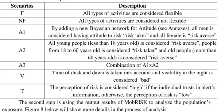
The new scenarios and how we named them are listed in Table 4 below, while their conditional probability tables are in Annexes:
12
Table 4: Name and description of the new scenarios
Scenarios Description
F All types of activities are considered flexible
NF All types of activities are considered not flexible
A1 By adding a new Bayesian network for Attitude (see Annexes), all men is considered having attitude to risk “risk taker” and all female is “risk averse” A2
All young people (less than 18 years old) is considered “risk averse”, people from 18 to 60 years old is considered “risk taker” and old people (more than
60 years old) is considered “risk averse”
A3 Combination of A1xA2
V Time of dusk and dawn is taken into account and visibility in the night is considered “bad”
T The perception of risk is considered “high” if the individual trusts in alert’s information, otherwise, the perception of risk is “low”
The second step is using the output results of MobRISK to analyze the population’s exposure. Figure 8 below will show more details in the process of analysis.
Figure 8: Calculation scheme
Twenty simulations of MobRISK are launched one at a time using the for loops in R. Each simulation usually takes about 1.5 minutes to 16 minutes, so it takes about 30 minutes to 5-6 hours to finish all 20 simulations. To shorten the time of execution, we tried using the
doParallel package with the foreach function, which allows the simulations to be executed in
parallel on multiple processors/cores of the computer (Weston and Calaway, 2017), the simulations can be run 5 at a time, so the running time is now about 20 minutes to 3 hours for all 20 simulations.
MASTER 2 TELENVI
13
5.2.Results of simulations and discussion
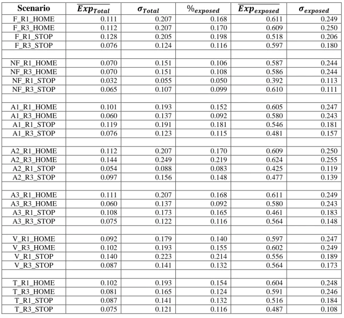
Table 5 below shows the results of analysis of the output of the model: the average exposure of the entire population ̅̅̅̅̅̅̅̅̅̅̅, standard deviation of the exposure , the percentage of the exposed people , the average exposure of the exposed people
̅̅̅̅̅̅̅̅̅̅̅̅̅̅, and its standard deviation .
Table 5: Results of the simulations
Scenario ̅̅̅̅̅̅̅̅̅̅̅ ̅̅̅̅̅̅̅̅̅̅̅̅̅̅ F_R1_HOME 0.111 0.207 0.168 0.611 0.249 F_R3_HOME 0.112 0.207 0.170 0.609 0.250 F_R1_STOP 0.128 0.205 0.198 0.518 0.206 F_R3_STOP 0.076 0.124 0.116 0.597 0.180 NF_R1_HOME 0.070 0.151 0.106 0.587 0.244 NF_R3_HOME 0.070 0.151 0.108 0.586 0.244 NF_R1_STOP 0.032 0.055 0.050 0.392 0.113 NF_R3_STOP 0.065 0.107 0.099 0.610 0.111 A1_R1_HOME 0.101 0.193 0.152 0.605 0.247 A1_R3_HOME 0.060 0.137 0.092 0.580 0.243 A1_R1_STOP 0.119 0.191 0.181 0.546 0.181 A1_R3_STOP 0.076 0.123 0.115 0.481 0.157 A2_R1_HOME 0.112 0.207 0.170 0.609 0.250 A2_R3_HOME 0.144 0.249 0.219 0.624 0.255 A2_R1_STOP 0.054 0.088 0.083 0.425 0.119 A2_R3_STOP 0.097 0.156 0.148 0.477 0.139 A3_R1_HOME 0.111 0.207 0.168 0.611 0.249 A3_R3_HOME 0.060 0.137 0.092 0.580 0.243 A3_R1_STOP 0.108 0.173 0.165 0.461 0.183 A3_R3_STOP 0.075 0.122 0.116 0.564 0.148 V_R1_HOME 0.092 0.179 0.140 0.597 0.247 V_R3_HOME 0.102 0.193 0.155 0.602 0.249 V_R1_STOP 0.140 0.223 0.214 0.556 0.189 V_R3_STOP 0.087 0.141 0.132 0.564 0.173 T_R1_HOME 0.102 0.193 0.154 0.604 0.248 T_R3_HOME 0.081 0.165 0.124 0.591 0.246 T_R1_STOP 0.087 0.141 0.132 0.516 0.184 T_R3_STOP 0.075 0.121 0.116 0.487 0.108
The results of the simulations show that motorists’ exposure of scenarios F are significantly larger than scenarios NF, which seems illogical with the conditional probability table where we defined the same values for both flexible and not flexible. Moreover, the scenarios A2_HOME (test the effect of age on attitude to risk) have the highest exposure among the scenarios done. However, the total standard deviation of the entire population is high, which means that there is a strong variability between simulations and between individuals.
14 On the other hand, according to Shabou (2016), the adoption of an overestimation of risk (“high risk perception”) will reduce the average exposure. Looking at the table of results above, we find that the scenario F, A1, A3, V_STOP, T follow this tendency but not the scenarios of NF, A2 and V_HOME.
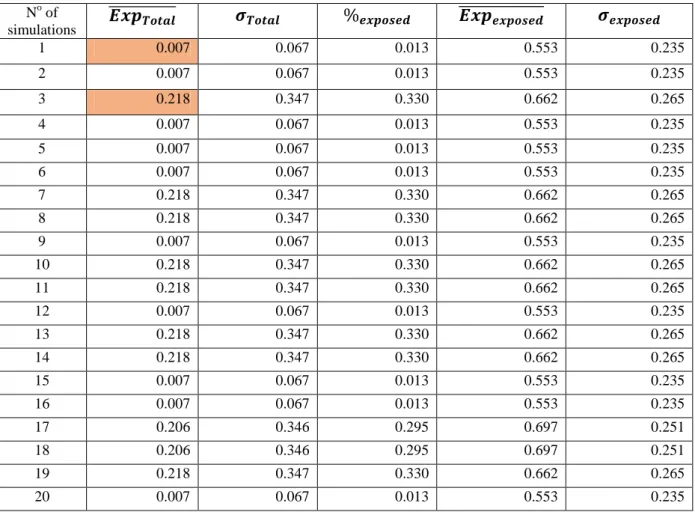
In order to understand the results of simulations, we tried to look more closely into the result each simulation. Firstly, looking at the analysis’s results of 20 simulations of the scenario F_R1_HOME (Table 6), we find that the variability of the exposure is very big, for example the first simulation gives us the average exposure of 0.007 but the third simulation is 0.218.
Table 6: Results of all 20 simulations of the scenario F_R1_HOME
No of simulations ̅̅̅̅̅̅̅̅̅̅̅ ̅̅̅̅̅̅̅̅̅̅̅̅̅̅ 1 0.007 0.067 0.013 0.553 0.235 2 0.007 0.067 0.013 0.553 0.235 3 0.218 0.347 0.330 0.662 0.265 4 0.007 0.067 0.013 0.553 0.235 5 0.007 0.067 0.013 0.553 0.235 6 0.007 0.067 0.013 0.553 0.235 7 0.218 0.347 0.330 0.662 0.265 8 0.218 0.347 0.330 0.662 0.265 9 0.007 0.067 0.013 0.553 0.235 10 0.218 0.347 0.330 0.662 0.265 11 0.218 0.347 0.330 0.662 0.265 12 0.007 0.067 0.013 0.553 0.235 13 0.218 0.347 0.330 0.662 0.265 14 0.218 0.347 0.330 0.662 0.265 15 0.007 0.067 0.013 0.553 0.235 16 0.007 0.067 0.013 0.553 0.235 17 0.206 0.346 0.295 0.697 0.251 18 0.206 0.346 0.295 0.697 0.251 19 0.218 0.347 0.330 0.662 0.265 20 0.007 0.067 0.013 0.553 0.235
We also tried to compare these two simulations spatially and temporally, Figure 9 shows the map of the simulated traffic load at road cuts during the flash flood event (8-9/9/2002). We can say that there is a considerable difference between the two simulations; the number of simulated traffic of the first simulation is a lot less than the third simulation.
MASTER 2 TELENVI
15
Figure 9: Spatially comparison of two simulation of scenario F_R1_HOME. The map above
is from the first simulation and the map below is from the third simulation.
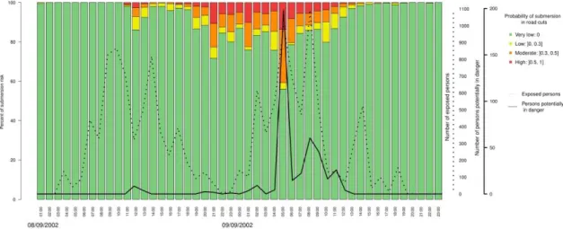
Concerning the temporal comparison of the two simulations, Figure 10 shows the result of this analysis. We find that the total number of exposed people (the dotted line) and number of people potentially in danger of the first simulation is no more than 1100 and 200 respectively, comparing to the third simulation with more than 40000 and 2100 respectively.
16
Figure 10: Spatially comparison of two simulation of scenario F_R1_HOME. The map above
is from the first simulation and the map below is from the third simulation.
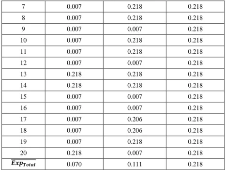
Secondly, we do the scenario F one more time but changing the conditional probability table driving the distribution of the HOME/KEEP-PLANNED and “STOP-DELAY/KEEP-PLANNED decisions. Scenario D1 refers to a larger tendency to go back HOME instead of KEEP PLANNED and scenario D5 is the opposite, D3 is the neutral scenario implemented earlier. The results are shown in Table 7.
Table 7: Comparison of the average exposure (ExpTotal) of 20 simulations for D1, D3 and
D5 for the decision HOME/KEEP PLANNED, a low risk perception (R1) and all activities considered as Flexible (F).
No of simulations
D1_F_R1_HOME D3_F_R1_HOME D5_F_R1_HOME
1 0.007 0.007 0.218 2 0.007 0.007 0.218 3 0.218 0.218 0.218 4 0.218 0.007 0.218 5 0.218 0.007 0.218 6 0.007 0.007 0.218
MASTER 2 TELENVI 17 7 0.007 0.218 0.218 8 0.007 0.218 0.218 9 0.007 0.007 0.218 10 0.007 0.218 0.218 11 0.007 0.218 0.218 12 0.007 0.007 0.218 13 0.218 0.218 0.218 14 0.218 0.218 0.218 15 0.007 0.007 0.218 16 0.007 0.007 0.218 17 0.007 0.206 0.218 18 0.007 0.206 0.218 19 0.007 0.218 0.218 20 0.218 0.007 0.218 ̅̅̅̅̅̅̅̅̅̅̅̅ 0.070 0.111 0.218
We find that although the probabilities of going back HOME or KEEP PLANNED change, the result of each simulation only varies between 2 values (0.007 and 0.218). The main difference between the D1, D3, D5 scenarios is that the value of 0.218 appears more frequently from D1 to D5, so that the total mean exposure ̅̅̅̅̅̅̅̅̅̅̅ also increases.
We think that when MobRISK chooses the route for the individuals, the model have chosen the exact same route for different simulations, in order to verify that hypothesis, we compare the itinerary of 1 individual between 2 simulations where is total exposure is similar. The comparison shows that the itinerary is the same if exposure is the same (Table 8 and 9). Note that the tables below just show the time, road-cut location and cumulated individual vulnerability for the day and for the event (2 days in the case of the 8-9 September flash flood) when the individual is confronted to a potentially submerged road cut.
Table 8: Comparison of simulation n°1 and n°2 for individual 1004570, with “time” is the
time that individual crosses road cuts, “location” is the code identity of the road cut; “daily_vulnerability” is the exposure of the individual calculated for one day and “event_vulnerability” is the exposure of the individual cumulated for the event period (exposure = 0.345)
Simulation n°1
time 2002-Sep-09 08:47:05 2002-Sep-09 08:47:12 2002-Sep-09 08:47:50 2002-Sep-09 08:47:55 location 2690 4017 2983 4637 daily_vulnerability 0.345 0.345 0.345 0.345 event_vulnerability 0.345 0.345 0.345 0.345 Simulation n°2
time 2002-Sep-09 08:46:44 2002-Sep-09 08:47:05 2002-Sep-09 08:47:12 2002-Sep-09 08:47:50 location 2690 4017 2983 4637 daily_vulnerability 0.345 0.345 0.345 0.345 event_vulnerability 0.345 0.345 0.345 0.345
18
Table 9: Comparison of simulation n°3 and n°7 (exposure = 0.1)
Simulation n°3
time 2002-Sep-09 11:57:57 2002-Sep-09 11:58:35 2002-Sep-09 11:58:40
loc 4017 2983 4637
daily_vulnerability 0.100 0.100 0.100 event_vulnerability 0.100 0.100 0.100 Simulation n°7
time 2002-Sep-09 11:57:57 2002-Sep-09 11:58:35 2002-Sep-09 11:58:40
loc 4017 2983 4637
daily_vulnerability 0.100000 0.100000 0.100000 event_vulnerability 0.100000 0.100000 0.100000
Third, we also compare the result given by running the simulations with the for loops with the foreach loops (Table 10). Even though the result still give the same tendency (exposure of R3 < R1), which is not corresponding with the result of Shabou (2016), we can find that the differences is pretty noticeable. Thus, the foreach loops which allows us to run 5 simulations in parallel (at the same time), may seem to run MobRISK not in the same way as the for loops.
Table 10: Comparison of results of simulations using the for loops and foreach loops for
scenario NF_R1_STOP and NF_R3_STOP
scenario ̅̅̅̅̅̅̅̅̅̅̅ ̅̅̅̅̅̅̅̅̅̅̅̅̅̅
foreach for foreach for foreach for foreach for foreach for
NF_R1 _STOP 0.032 0.087 0.055 0.141 0.050 0.132 0.391 0.585 0.113 0.130 NF_R3 _STOP 0.065 0.098 0.107 0.157 0.099 0.148 0.610 0.509 0.111 0.138
Finally, when comparing the average exposure ̅̅̅̅̅̅̅̅̅̅̅ result of scenario R1_HOME
of each scenario (F, NF, A1, A2, A3, V, T) (Table 11), the exposure also seem to give only three values 0.218; 0.206 or 0.007. Hence, we think that the changes of the parameters in the decision-making model somehow are too small and cannot make a difference to the final average values of the exposure.
Table 11: Comparison of the average exposure of all 20 simulations result of scenario
D3_R1_HOME of each scenario (F, NF, A1, A2, A3, V, T) N° of simulation R1_HOME F NF A1 A2 A3 V T 1 0.007 0.007 0.206 0.218 0.007 0.007 0.218 2 0.007 0.007 0.218 0.218 0.007 0.218 0.218 3 0.218 0.206 0.007 0.007 0.007 0.007 0.007 4 0.007 0.007 0.007 0.218 0.218 0.007 0.007 5 0.007 0.007 0.218 0.007 0.007 0.007 0.007 6 0.007 0.007 0.007 0.007 0.007 0.007 0.007 7 0.218 0.007 0.218 0.007 0.007 0.007 0.007
MASTER 2 TELENVI 19 8 0.218 0.007 0.007 0.218 0.206 0.007 0.218 9 0.007 0.218 0.007 0.206 0.218 0.007 0.218 10 0.218 0.007 0.218 0.218 0.007 0.007 0.218 11 0.218 0.007 0.007 0.007 0.218 0.218 0.007 12 0.007 0.218 0.007 0.007 0.218 0.218 0.007 13 0.218 0.218 0.218 0.007 0.007 0.218 0.206 14 0.218 0.007 0.007 0.218 0.218 0.218 0.218 15 0.007 0.218 0.007 0.218 0.218 0.218 0.007 16 0.007 0.007 0.007 0.007 0.218 0.007 0.007 17 0.206 0.007 0.218 0.007 0.218 0.007 0.007 18 0.206 0.218 0.218 0.218 0.007 0.218 0.007 19 0.218 0.007 0.007 0.007 0.206 0.218 0.218 20 0.007 0.007 0.206 0.218 0.007 0.007 0.218 6. Conclusion
This report is about understanding and exploits the MobRISK model, developed to measure the exposure of motorists to road submersion in flash floods events, the model integrating the mobility’s simulation component, the environmental simulation component and the mobility adaptation decisions component which can simulate individual’s decision in flash flooding events. The model allows us to analyze the spatial and temporal dynamics of simulated traffic flow and submersion probability, so that we also know the spatial-temporal dynamics of exposure in the flash flood event periods. The first application of the model is conducted in the Alès area of the Gard department in southern of France for the flash flood event on 8-9 September 2002. MobRISK has been proved that has many potentialities and can be applied to road management, security operations, psychology research, etc.
However, the results of exploitation the decision-making components of MobRISK show that this components still need some improvements: (i) there is a big variation between the average exposures of the simulations in each scenario, which is possibly related to the simulation of the mobility which involved too much randomness in the location of the destinations of the individuals; (ii) the use of the foreach function in order to improve the time of calculation of MobRISK might not be the best way; and (iii) the changes of the parameters in the Bayesian network of the decision-making model have not really affected the final result.
The next steps of this research will have to continue to understand and explain the results of the simulations by playing with the parameters entered in the decision conditional probability table to change the weight of different variables in the final decision to KEEP_PLANNED or go HOME. It would also be interesting to investigate further ways to reduce the variability of the total exposure between simulations of the same scenarios.
20 List of figures
Figure 1: Results of implementation of the decision-making component into MobRISK
(Shabou, 2016) ... 2
Figure 2: Map of the study area around Alès ... 4
Figure 3: Architecture of MobRISK (Shabou, 2016) ... 7
Figure 4: Bayesian network of Bottleneck event (Shabou, 2016) ... 8
Figure 5: Bayesian network of Broadcast event (Shabou, 2016) ... 8
Figure 6: Bayesian network of Environment cue event (Shabou, 2016) ... 9
Figure 7: Bayesian network of End of activity event (Shabou, 2016) ... 9
Figure 8: Calculation scheme ... 12
Figure 9: Spatially comparison of two simulation of scenario F_R1_HOME. The map above is from the first simulation and the map below is from the third simulation. ... 15
Figure 10: Spatially comparison of two simulation of scenario F_R1_HOME. The map above is from the first simulation and the map below is from the third simulation. ... 16
MASTER 2 TELENVI
21 List of tables
Table 1: Geographical input data of MobRISK ... 5
Table 2: Probability of submersion associated with different sensibility classes according to the return period of peak flow (Naulin et al., 2012) ... 6
Table 3: Social input data of MobRISK ... 6
Table 4: Name and description of the new scenarios ... 12
Table 5: Results of the simulations ... 13
Table 6: Results of all 20 simulations of the scenario F_R1_HOME ... 14
Table 7: Comparison of the average exposure (ExpTotal) of 20 simulations for D1, D3 and D5 for the decision HOME/KEEP PLANNED, a low risk perception (R1) and all activities considered as Flexible (F). ... 16
Table 8: Comparison of simulation n°1 and n°2 for individual 1004570, with “time” is the time that individual crosses road cuts, “location” is the code identity of the road cut; “daily_vulnerability” is the exposure of the individual calculated for one day and “event_vulnerability” is the exposure of the individual cumulated for the event period (exposure = 0.345) ... 17
Table 9: Comparison of simulation n°3 and n°7 (exposure = 0.1) ... 18
Table 10: Comparison of results of simulations using the for loops and foreach loops for scenario NF_R1_STOP and NF_R3_STOP ... 18
Table 11: Comparison of the average exposure of all 20 simulations result of scenario D3_R1_HOME of each scenario (F, NF, A1, A2, A3, V, T) ... 18
22 References
Antoine, J.-M. D. (2001). Les crues meurtrières, du roussillon aux cévennes/casualty-causing flood : from the roussillon region to the cevennes country. Annales de géographie, 597–623.
Coates, L. (1999). Flood fatalities in Australia, 1788-1996. Australian Geographer, 30(3), 391-408.
Cools, M., & Creemers, L. (2013). The dual role of weather forecasts on changes in activity-travel behavior. Journal of Transport Geography, 28, 167-175.
Delrieu, G., Nicol, J., Yates, E., Kirstetter, P.-E., Creutin, J.-D., Anquetin, S., . . . Ducrocq, V. G. (2005). The castastrophic flash-flood event of 8-9 september 2002 in the Gard region, France: A first case study for the cevennes-vivarais mediterranean hydrometeorological observatory. Journal of Hydrometeorology, 6(1), 34-52.
Jonkman, S., & Kelman, I. (2005). An analysis of the causes and circumstances of flood disaster deaths. Disasters, 29(1), 75-97.
Kilpeläïnen, M., & Summala, H. (2007). Effects of weather and weather forecasts on driver behaviour. Transportation research part F: traffic psychology and behaviour, 10(4), 288-299.
Mileti, D. (1995). Factors related to flood warning response. US-Italy Research Workshop on
the Hydrometerology, Impacts, and Management of Extreme Floods, 1-17.
Montz, B. E., & Grunfest, E. (2002). Flash flood mitigation: recommendations for research and applications. Global Environmental Change Part B: Environmental Hazards 4(1), 15-22.
Naulin, J.-P., Payrastre, O., & Gaume, E. (2013). Spatially distributed flood forecasting in flash flood prone areas : Application to road network supervision in Southern France.
Journal of hydrology, 486, 88-99.
Ruin, I. (2007). Conduite à contre-courant. Les pratiques de mobilité dans le Gard: facteur de vulnérabilité aux crues rapides. PhD Thesis.
Ruin, I., Creutin, J.-D., Anquetin, S., & Lutoff, C. (2008). Human exposure to flash floods – Relation between flood parameters and human vulnerability during a storm of September 2002 in Southern France. Journal of Hydrology, 361(1), 199-213.
Ruin, I., Lutoff, C., Boudevillain B., C. J.-D., Anquetin, S., B., R. M., Boissier, L., . . . O., P. (2014). Social and Hydrological Responses to Extreme Precipitations: An Interdisciplinary. Weather, climate, and society, 6(1), 135-153.
Shabou, S. (2016). Extrême hydro-métorologiques & Exposition dur les routes. Contribution à MobRISK: Modèle de simulation de l'exposition des mobilités quotidiennes aux crues rapides. PhD thesis.
MASTER 2 TELENVI
23 Shabou, S., Ruin, I., Lutoff, C., Debionne, S., Anquetin, S., Creutin, J.-D., & Beaufils, X. (2017). MobRISK: a model for assessing the exposure of road users to flash flood events. Natural Hazards and Earth System Sciences, 17, 1631-1651.
Studer, M., Ritschard, G., Gabadinho, A., & Müller, N. S. (2011). Discrepancy analysis of state sequences. Sociological Methods & Research, 40(3), 471–510.
Terti, G., Ruin, I., Anquetin, S., & Gourley, J. (2017). A situation-based analysis of flash flood fatalities in the United States. Bulletin of the American Meteorological Society,
98, 333-345.
Terti, G., Ruin, I., Anquetin, S., & J., G. J. (2015). Dynamic vulnerability factors for impact-based flash flood prediction. Natural Hazards, 79(3), 1481-1497.
Vannier, O. A. (2016). Investigating the role of geology in the hydrological response of Mediterranean catchments prone to flash-floods: regional modelling study and process understanding. Journal of Hydrology, 541, 158-172.
Versini, P.-A. G. (2010). Assessment of the susceptibility of roads to flooding based on geographical information–test in a flash flood prone area (the Gard region, France).
Natural Hazards and Earth System Science, 10(4), 793-803.
Weston, S., & Calaway, R. (2017). Getting started with doParallel and foreach.
24 Annexes
Tables of Conditional probability
Common tables: these tables are the same for all the scenarios (F, NF, A1, A2, A3, except scenario V and T)
1. Scenario D3_R1
1.1.Decision STOP
1.1.1. Bottleneck event
Visibility: P(visibility | luminosity, rain)
luminosity day night dusk_dawn
rain low medium high low medium high low medium high visibility good 0.8 0.5 0.3 0.4 0.2 0 0.4 0.2 0
bad 0.2 0.5 0.7 0.6 0.8 1 0.6 0.8 1
Risk: P(risk | visibility, submersion)
visibility good bad
submersion low medium high low medium high
risk low 1 1 1 1 1 1
medium 0 0 0 0 0 0
high 0 0 0 0 0 0
Decision: P(decision | risk, flexibility, attitude)
risk low medium high
flexibility flexbible not flexible flexbible not flexible flexbible not flexible attitude take avoid take avoid take avoid take avoid take avoid take avoid deci sion keep planned 0.5 0.5 0.5 0.5 0.5 0.5 0.5 0.5 0.5 0.5 0.5 0.5 skip 0 0 0 0 0 0 0 0 0 0 0 0 home 0 0 0 0 0 0 0 0 0 0 0 0 stop 0.5 0.5 0.5 0.5 0.5 0.5 0.5 0.5 0.5 0.5 0.5 0.5 1.1.2. Broadcast event
Broadcast_trust: P(broadcast_trust | type, trust)
source Meteo_france Other
trust yes no yes no
Broadcast_trust yes 1 0 0.8 0.2
MASTER 2 TELENVI
25 Perception: P(perception | situation)
situation at_home out_home on_road perception yes 0.8 0.2 0.5
no 0.2 0.8 0.5
Risk: P(risk | perception, level, broadcast_trust)
perception yes no
level low medium high low medium high broadcast_trust yes no yes no yes no yes no yes no yes no ris
k
low 1 1 1 1 1 1 1 1 1 1 1 1 medium 0 0 0 0 0 0 0 0 0 0 0 0 high 0 0 0 0 0 0 0 0 0 0 0 0
Decision: P(decision | risk, flexibility, situation)
risk low medium high
flexibility flexbible not_flex flexbible not_flex flexbible not_flex situation at ho me out ho me on ro ad at ho me out ho me on ro ad at ho me out ho me on ro ad at ho me out ho me on ro ad at ho me out ho me on ro ad at ho me out ho me on ro ad de ci si on kee p curr ent 0.5 0.5 0. 5 0.5 0.5 0. 5 0.5 0.5 0. 5 0.5 0.5 0. 5 0.5 0.5 0. 5 0.5 0.5 0. 5 ho me 0.5 0.5 0. 5 0.5 0.5 0. 5 0.5 0.5 0. 5 0.5 0.5 0. 5 0.5 0.5 0. 5 0.5 0.5 0. 5
1.1.3. Environment cue event Risk: P(risk| level, situation)
type rain other
level low medium high low medium high situation at ho me out ho me on ro ad at ho me out ho me on ro ad at ho me out ho me on ro ad at ho me out ho me on ro ad at ho me out ho me on ro ad at ho me out ho me on ro ad ri s k low 1 1 1 1 1 1 1 1 1 1 1 1 1 1 1 1 1 1 medi um 0 0 0 0 0 0 0 0 0 0 0 0 0 0 0 0 0 0 high 0 0 0 0 0 0 0 0 0 0 0 0 0 0 0 0 0 0
Decision: P(decision | risk, flexibility, situation)
risk low medium high
flexibility flexbible not_flex flexbible not_flex flexbible not_flex situation at ho me out ho me on ro ad at ho me out ho me on ro ad at ho me out ho me on ro ad at ho me out ho me on ro ad at ho me out ho me on ro ad at ho me out ho me on ro ad de ci kee p 0.5 0.5 0. 5 0.5 0.5 0. 5 0.5 0.5 0. 5 0.5 0.5 0. 5 0.5 0.5 0. 5 0.5 0.5 0. 5
26 si on curr ent ho me 0.5 0.5 0. 5 0.5 0.5 0. 5 0.5 0.5 0. 5 0.5 0.5 0. 5 0.5 0.5 0. 5 0.5 0.5 0. 5
1.1.4. End of activity event Risk: P(risk | rain, luminosity)
rain low medium high
luminosity day night dusk_dawn day night dusk_dawn day night dusk_dawn
risk low 1 1 1 1 1 1 1 1 1
medium 0 0 0 0 0 0 0 0 0
high 0 0 0 0 0 0 0 0 0
Decision: P(decision | risk, flexibility, attitude)
risk low medium high
flexibility flexbible not flexible flexbible not flexible flexbible not flexible attitude take avoid take avoid take avoid take avoid take avoid take avoid deci sion keep planned 0.5 0.5 0.5 0.5 0.5 0.5 0.5 0.5 0.5 0.5 0.5 0.5 delay 0.5 0.5 0.5 0.5 0.5 0.5 0.5 0.5 0.5 0.5 0.5 0.5 skip 0 0 0 0 0 0 0 0 0 0 0 0 home 0 0 0 0 0 0 0 0 0 0 0 0 1.2.Decision HOME 1.2.1. Bottleneck event
Decision: P(decision | risk, flexibility, attitude)
risk low medium high
flexibility flexbible not flexible flexbible not flexible flexbible not flexible attitude take avoid take avoid take avoid take avoid take avoid take avoid deci sion keep planned 0.5 0.5 0.5 0.5 0.5 0.5 0.5 0.5 0.5 0.5 0.5 0.5 skip 0 0 0 0 0 0 0 0 0 0 0 0 home 0.5 0.5 0.5 0.5 0.5 0.5 0.5 0.5 0.5 0.5 0.5 0.5 stop 0 0 0 0 0 0 0 0 0 0 0 0 1.2.2. Broadcast event
Decision: P(decision | risk, flexibility, situation)
risk low medium high
flexibility flexbible not_flex flexbible not_flex flexbible not_flex situation at ho me out ho me on ro ad at ho me out ho me on ro ad at ho me out ho me on ro ad at ho me out ho me on ro ad at ho me out ho me on ro ad at ho me out ho me on ro ad de kee 0.5 0.5 0. 0.5 0.5 0. 0.5 0.5 0. 0.5 0.5 0. 0.5 0.5 0. 0.5 0.5 0.
MASTER 2 TELENVI 27 ci si on p curr ent 5 5 5 5 5 5 ho me 0.5 0.5 0. 5 0.5 0.5 0. 5 0.5 0.5 0. 5 0.5 0.5 0. 5 0.5 0.5 0. 5 0.5 0.5 0. 5
1.2.3. Environment cue event Decision: P(decision | risk, flexibility, situation)
risk low medium high
flexibility flexbible not_flex flexbible not_flex flexbible not_flex situation at ho me out ho me on ro ad at ho me out ho me on ro ad at ho me out ho me on ro ad at ho me out ho me on ro ad at ho me out ho me on ro ad at ho me out ho me on ro ad de ci si on kee p curr ent 0.5 0.5 0. 5 0.5 0.5 0. 5 0.5 0.5 0. 5 0.5 0.5 0. 5 0.5 0.5 0. 5 0.5 0.5 0. 5 ho me 0.5 0.5 0. 5 0.5 0.5 0. 5 0.5 0.5 0. 5 0.5 0.5 0. 5 0.5 0.5 0. 5 0.5 0.5 0. 5
1.2.4. End of activity event
Decision: P(decision | risk, flexibility, attitude)
risk low medium high
flexibility flexbible not flexible flexbible not flexible flexbible not flexible attitude take avoid take avoid take avoid take avoid take avoid take avoid deci sion keep planned 0.5 0.5 0.5 0.5 0.5 0.5 0.5 0.5 0.5 0.5 0.5 0.5 delay 0 0 0 0 0 0 0 0 0 0 0 0 skip 0 0 0 0 0 0 0 0 0 0 0 0 home 0.5 0.5 0.5 0.5 0.5 0.5 0.5 0.5 0.5 0.5 0.5 0.5
2. Scenario D3_R3: this scenario is basically the same with scenario R1, except the
table of risk perception where the level is “high” (in R1, the level is “low”) 2.1.Bottleneck event
P(risk | visibility, submersion)
visibility good bad
submersion low medium high low medium high
risk low 0 0 0 0 0 0
medium 0 0 0 0 0 0
28 2.2.Broadcast event
P(risk | perception, level, broadcast_trust)
perception yes no
level low medium high low medium high broadcast_trust yes no yes no yes no yes no yes no yes no risk low 1 1 1 1 1 1 1 1 1 1 1 1
medium 0 0 0 0 0 0 0 0 0 0 0 0 high 0 0 0 0 0 0 0 0 0 0 0 0
2.3.Environment cue event P(risk| level, situation)
type rain other
level low medium high low medium high situation at ho me out ho me on ro ad at ho me out ho me on ro ad at ho me out ho me on ro ad at ho me out ho me on ro ad at ho me out ho me on ro ad at ho me out ho me on ro ad ri s k low 1 1 1 1 1 1 1 1 1 1 1 1 1 1 1 1 1 1 medi um 0 0 0 0 0 0 0 0 0 0 0 0 0 0 0 0 0 0 high 0 0 0 0 0 0 0 0 0 0 0 0 0 0 0 0 0 0
2.4.End of activity event P(risk | rain, luminosity)
rain low medium high
luminosity day night dusk_dawn day night dusk_dawn day night dusk_dawn
risk low 1 1 1 1 1 1 1 1 1
medium 0 0 0 0 0 0 0 0 0
high 0 0 0 0 0 0 0 0 0
3. Scenario D1 and D5: These 2 scenarios are different from scenario D3 in the
Decision table of each event. For example in Bottleneck event:
Scenario D1:
risk low medium high
flexibility flexbible not flexible flexbible not flexible flexbible not flexible attitude take avoid take avoid take avoid take avoid take avoid take avoid decisio n keep planne d 0,25 0,25 0,25 0,25 0,125 0,125 0,125 0,125 0 0 0 0 skip 0 0 0 0 0 0 0 0 0 0 0 0 home 0 0 0 0 0 0 0 0 0 0 0 0 stop 0,75 0,75 0,75 0,75 0,875 0,875 0,875 0,875 1 1 1 1
MASTER 2 TELENVI
29
Scenario D5
risk low medium high
flexibility flexbible not flexible flexbible not flexible flexbible not flexible attitude take avoid take avoid take avoid take avoid take avoid take avoid decision keep planned 1 1 1 1 0,875 0,87 5 0,87 5 0,87 5 0,75 0,75 0,75 0,75 skip 0 0 0 0 0 0 0 0 0 0 0 0 home 0 0 0 0 0 0 0 0 0 0 0 0 stop 0 0 0 0 0,125 0,12 5 0,12 5 0,12 5 0,25 0,25 0,25 0,25
4. Scenario F: in this scenario, all the activities are flexible in all 4 events.
Flexibility: P(flexibility | activity)
activity 1 home 2 shop ping 3 medic al 4 administrati ve 5 visitin g 6 accompanyi ng 7 leisur e 8 holiday s 9 work 10 study flexibili ty flex 1 1 1 1 1 1 1 1 1 1 not_flex 0 0 0 0 0 0 0 0 0 0
Scenario NF: all the activities are not flexible in all 4 events.
Flexibility: P(flexibility | activity)
activity 1 home 2 shoppi ng 3 medic al 4 administrati ve 5 visitin g 6 accompanyi ng 7 leisur e 8 holida ys 9 work 10 study flexibili ty flex 0 0 0 0 0 0 0 0 0 0 not_fl ex 1 1 1 1 1 1 1 1 1 1
5. Bayesian network of Attitude
To test the effect of age and sex of individual, we have to create the Bayesian network for Attitude: