O
pen
A
rchive
T
OULOUSE
A
rchive
O
uverte (
OATAO
)
OATAO is an open access repository that collects the work of Toulouse researchers and makes it freely available over the web where possible.This is an author-deposited version published in : http://oatao.univ-toulouse.fr/ Eprints ID : 13869
To link to this article : DOI: 10.1080/02626667.2014.909596 URL :http://dx.doi.org/10.1080/02626667.2014.909596
To cite this version : Garambois, Pierre-André and Roux, Hélène and Larnier, Kévin and Labat, David and Dartus, Denis Characterization of catchment behaviour and rainfall selection for flash flood
hydrological model calibration: catchments of the eastern Pyrenees. (2015) Hydrological sciences journal, vol. 60 (n° 3). pp. 424-447. ISSN 0262-6667
Any correspondance concerning this service should be sent to the repository administrator: [email protected]
Characterization of catchment behaviour and rainfall selection for flash
flood hydrological model calibration: catchments of the eastern
Pyrenees
P.A. Garambois1,2, H. Roux1,2, K. Larnier1,2, D. Labat1,3 and D. Dartus1,2
1Université de Toulouse, INPT, UPS, IMFT (Institut de Mécanique des Fluides de Toulouse), F-31400 Toulouse, France 2
CNRS, IMFT, F-31400 Toulouse, France
3
Géosciences Environnement Toulouse, Université de Toulouse-CNRS-IRD-OMP, F-31400 Toulouse, France
Abstract Accurate flash flood prediction depends heavily on rainfall data quality and knowledge of catchment behaviour. A methodology based on global sensitivity analysis and hydrological similarity is proposed to analyse flash storm-flood events with a mechanistic model. The behaviour of medium-sized catchments is identified in terms of rainfall–runoff conservation. On the basis of this shared behaviour, rainfall products with questionable quantitative precipitation estimation (QPE) are excluded. This facilitates selection of rainfall inputs for calibra-tion, whereas it can be difficult to choose between two rainfall products by direct comparison. A substantial database of 43 flood events on 11 catchment areas was studied. Nash-Sutcliffe efficiencies for this dataset are around 0.9 in calibration and 0.7 in validation for flash flood simulation in 250-km2 catchments with selected QPE. The resulting calibration framework and qualification of possible losses for different bedrock types are also interesting bases for flash flood prediction at ungauged locations.
Key words flash floods; global sensitivity analysis; catchment behaviour; QPE; hydrological model calibration; regionalization; bedrock loss
Caractérisation de comportements de bassins versants et sélection de pluies pour la calibration de modèles hydrologiques dans le cas de crues éclair : bassins de l’est des Pyrénées
Résumé La précision des prévisions de crues éclair dépend largement de la qualité des données de pluie et de la connaissance du comportement des bassins versants. Une méthodologie basée sur de l’analyse de sensibilité globale et des similarités hydrologiques est proposée afin d’analyser des évènements de crues éclair à l’aide d’un modèle pluie débit mécaniste. Le comportement de bassins versants de taille moyenne est identifié en termes de conservation du volume d’eau entre la pluie et le débit. A partir d’un comportement hydrologique, les produits de pluie présentant des estimations quantitatives de précipitation (EQP) douteuses sont exclus. Ainsi, la sélection de données de pluie pour la calage est facilitée alors qu’il peut être difficile de choisir un produit de pluie plutôt qu’un autre par une comparaison directe. Une base de données conséquente et composée de 43 évènements de crues sur 11 bassins versants a été étudiée. Les performances (Nash) sont de l’ordre de 0,9 en calage et de 0,7 en validation pour des crues éclair survenues sur des bassins de 250 km2et modélisées à l’aide d’EQP sélectionnées. La méthode de caage et l’identification de pertes potentielles vers le socle rocheux sont des bases intéressantes pour la prévision de crues éclair sur des bassins non jaugés.
Mots clefs crue éclair ; analyse de sensibilité globale ; comportement hydrologique de bassin versant ; EQP ; calage de modèle hydrologique ; régionalisation ; perte vers le socle rocheux
1 INTRODUCTION: PROBLEM FRAMEWORK
Like the storms that cause them, flash floods are very variable and nonlinear phenomena in time and space, with the result that understanding and anticipating
flash flood genesis is far from straightforward. Flash floods are generally triggered by intense and localized storms, and water depth in the drainage network can reach peak levels in a few minutes or a few hours (Georgakakos 1992). Monitoring flash
floods is particularly difficult (Borga et al. 2008), as conventional measurement networks monitoring rain-fall and river discharges cannot sample effectively due to problems of scale (Creutin and Borga 2003). That is why hydrological forecasts focus increasingly on remote sensing techniques, such as radar (Krajewski and Smith 2002), high-resolution hydro-meteorological prediction models (Seity et al. 2011, Vincendon et al.2010,2011), knowledge of climatic antecedents of a catchment or region and initializa-tion of event models (Tramblay et al. 2010, Roux et al. 2011). Taking into account the uncertainty due to the model structure itself or to spatio–temporal rainfall is recognized as important in hydrological modelling (Kirstetter et al. 2010, Delrieu et al. 2014). As highlighted by Looper and Vieux (2012), flood prediction accuracy is linked to the quality of rainfall estimates and forecasts. The robustness of rainfall–runoff models might be increased and knowledge of uncertainty might be improved by the availability, the anteriority and the quality of hydro-meteorological time series, and, in several cases, by their space–time resolution.
Estimated precipitation can be considered as one of the most important inputs required for hydrologi-cal prediction. Rainfall distribution and amount deter-mine surface hydrological processes and therefore catchment response dynamics. An adequate charac-terization of rainfall input is fundamental for success in rainfall–runoff modelling: no model, however well founded in physical theory or empirically justified by past performance, can produce accurate runoff pre-dictions forced by inaccurate rainfall data (e.g. Beven 2002, Moulin et al.2009).
Although radar-based weather coverage has increased considerably over the last two decades enabling high-resolution spatial and temporal mea-surements of rainfall, quantitative precipitation esti-mation (QPE) still presents difficulties due to the limitations of radar measurements. Radar QPE there-fore still currently relies strongly on gauge measurements.
An important question is how many raingauges are needed to get a correct QPE and to model error, or what radar-to-gauge ratio is required? In the case of catchment hydrology the underlying question is: does the proportion of the rainfall measured by the raingauge network explain most of the hydrological response, and with what accuracy? Indeed the sig-nificance of in situ measurements can be directly affected by catchment rainfall space–time dynamics (Viglione et al. 2010, Zoccatelli et al. 2011). For
instance, the speed and direction of movement of rain cells seem to exert a strong control on the hydro-logical response of an arid catchment (Yakir and Morin2011).
However, rainfall estimation errors, like other sources of uncertainty, can be mainly compensated by hydrological model parameter values often deter-mined through a calibration process. Bárdossy and Das (2008) show that the semi-distributed HBV model using different rainfall measurement networks needs to be recalibrated. Specifically they state that calibration of the model with relatively sparse rainfall data leads to good performance with dense precipita-tion measurement, while the model calibrated on dense precipitation information fails on sparse data. There are several studies of Mediterranean flash floods at the regional scale in the literature. Ayral et al. (2007), with the ALTHAIR model, and Le Lay and Saulnier (2007), with the event-based TOPMODEL approach, tested different levels of sophistication in the regionalization of inputs and model parameters. Ayral et al. (2007) obtained a systematic overestimate of peak discharge and a satisfactory simulation of the time of the peak when the model was used with spatially homogeneous parameters. Le Lay and Saulnier (2007) show that the efficiency of the model significantly increases when the spatial variability of rainfall is taken into account. Nevertheless, for some catchments the per-formance failures remain unexplained. Tramblay et al. (2011) used soil moisture initialization with
SIM data (SAFRAN-ISBA-MODCOU; Habets
et al. 2008) and show the benefit of using spatial radar to measure rainfall on the Gardon d’Anduze catchment (545 km2) in the Cévennes region, France, particularly for the largest flood events. Versini (2012) shows that in the Gard region, France, the predictive power of a road submersion system in cases of flash floods is affected by rainfall uncer-tainty which drastically drops for lead times exceed-ing two hours. The effects of uncertainty in the rainfall forecast are highlighted by a recent study in the Besos River basin, Catalonia, Spain (Quintero et al. 2012). However, little information can be found in the literature about the calibration of flash flood models and the problem of rainfall uncertainty. The problem of rainfall uncertainty is particu-larly crucial when attempting to develop flash flood regionalization methodologies, especially on fast-responding catchments involving several difficult problems, such as structural, parametric or data uncertainties. Regionalization of model parameters
to ungauged catchments is generally performed on the basis of knowledge acquired from modelling on gauged catchments (Merz and Blöschl 2004, Wagener et al. 2004, Blöschl 2005). Different approaches may give considerably different results, particularly if unusual conditions prevail, e.g. regard-ing soil, geology, or climatology (Weregard-ingartner et al. 2003). For this reason, it is particularly important to understand catchment response through a sensitivity analysis of model parameters. Sensitivity analysis that assesses the impact of model parameters on the output is indeed a convenient tool for investigating model behaviour and particularly the importance of certain choices of parameterization within the model. It is possible to explore high-dimensional parameter space and some studies show the usefulness of sensi-tivity analysis for hydrological model improvement (Andréassian et al. 2001, Oudin et al. 2006, Tang et al. 2007, Pushpalatha et al. 2011), or to better understand model behaviour with respect to inputs such as precipitation (Xu et al.2006, Meselhe et al. 2009).
Hydrological models are characterized by com-plex response surfaces due to the mathematical for-mulation used to describe the rainfall–runoff phenomenon. It can therefore be difficult to deter-mine optimal parameter combinations given multiple convergence zones, anisotropic curving, or singular points responsible for discontinuities of derivatives (Johnston and Pilgrim 1976, Duan et al.1992). This poses the problem of local extrema for both calibra-tion and sensitivity analysis. In this context, global sensitivity analysis methods, unlike local ones, have been proposed for examining multiple locations in the physically possible parameter space. Regional sensitivity analysis (RSA) was originally developed by Hornberger and Spear (1981) and later called generalized sensitivity analysis (GSA) by Freer et al. (1996) in the context of environmental model-ling to reduce the number of model parameters. This approach is particularly important with the current shift towards distributed hydrological models. In the case of flash flood event modelling, it is indeed interesting to perform an analysis of the sensitivity of model outputs to parameter variations over large ranges. The GSA method is a global approach. It tackles the question of sensitivity by sampling the space of uncertain model inputs (parametric uncer-tainty is usually considered) in order to enable the conditioning of model predictions on available obser-vations using a likelihood measure (Beven and Binley 1992).
Understanding the sources of uncertainty is cur-rently a central question in hydrology. This can be achieved by various methods, of which formal Bayesian methods (Kuczera and Parent 1998) and the generalized likelihood uncertainty estimation (GLUE) method (Beven and Binley 1992) are the most popular, along with recursive application of GSA for dynamic identifiability analysis (Wagener et al. 2003) or Bayesian total error analysis (Kavetski et al. 2006) for comprehensive calibration and uncertainty estimation. They have been widely discussed with respect to their philosophy and the mathematical rigour on which they rely (Gupta et al. 2003, Beven 2006, Mantovan and Todini 2006, Todini 2007, Beven et al. 2008, Yang et al. 2008, Vrugt et al.2009, Jin et al.2010, Yang2011). These contributions show that results of the GLUE method are notably influenced by threshold values on the cost function and parameter variation ranges (Yang et al.2008, Yang2011). In addition, Li et al. (2010) performed a comprehensive evaluation of the para-meters and total uncertainty estimated by GLUE and a formal Bayesian approach to quantify the conse-quences of (a) threshold values or the acceptable sample rate (ASR), and (b) the number of sample simulations on the results of GLUE.
Moreover, the need to define limits of accept-ability before model runs when applying the GLUE methodology is highlighted in Beven (2006). For example, limits of acceptability for discharge are defined using an estimated rating curve error at five sites within the Skalka catchment in the Czech Republic, and then relaxed to allow a strong realiza-tion effect in predicted flood frequencies (Blazkova and Beven2009).
In this study we focus on the quality of the rainfall estimate for rainfall–runoff modelling and the selection of calibration events for the regionaliza-tion of flash flood models. Indeed for regionalizaregionaliza-tion, a rainfall–runoff model may need to be calibrated on gauged catchments. This raises the questions: How do we select the calibration/validation events? Should all possible events be used? What about the intrinsic quality of the mean areal precipitation for each event and its impact on the estimated values of the para-meters? For the catchments of interest in the Mediterranean region, several rainfall products are often available and for most events it is difficult to choose between them using direct comparison of the different rainfall products. This study proposes a methodology using sensitivity analysis of the MARINE rainfall–runoff model, dedicated to flash
flood analysis and forecasting in the Mediterranean region (Roux et al.2011). Based on the results of this sensitivity analysis, water conservation controls and simulated runoff coefficients are explored. In particu-lar, cumulative distribution functions of the para-meters often show mean catchment behaviours, which help to select flash flood events for model calibration. This enables rainfall products with ques-tionable QPE to be excluded. The aim is to prepare the calibration of catchment parameter sets and reduce the significant uncertainty introduced by rain-fall QPE data in the case of flash flood modelling. The chosen catchments possess contrasting physio-graphic properties, thus helping to provide a holistic understanding of hydrological controls (Gaál et al. 2012).
The present paper is organized as follows. Section 2 is a presentation of the study zone and the catalogue of catchments and events considered, with some characteristics of soils and geology for comparative general sensitivity analysis. Section 3 briefly presents the MARINE model and its hypoth-esis. Section 4investigates the influence of different radar or interpolated rainfall products measured with raingauges on model calibration and sensitivities, particularly for soil volume.Section 5presents catch-ment parameter sets calculated with a multiple event
calibration method, with, for each event selected, the best rainfall products by comparing their respective sensitivities. Finally, Section 6 presents a discussion on modelling performance and the resulting under-standing of hydrological processes, regarded as a first essential step towards prediction of flash floods in ungauged catchments.
2 STUDY ZONE AND CATCHMENT PROPERTIES
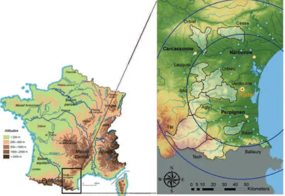
The proximity of the Mediterranean Sea and the steep surrounding topography can promote low level uplifting in an unstable atmosphere, as for example in the Alps and Pyrenees (Davolio et al.2009, Tarolli et al. 2012). The region of interest is thus fairly frequently affected by intense rainfall, and represents an interesting area for regional studies of flash floods, considering the number of small to medium-sized responding catchments. The dataset for this study is composed of 11 catchments in the foothills of the eastern Pyrenees with areas ranging from 36 to 776 km2 (Fig. 1), representing a significant number of flood events (43) ranging from moderate flood to strong flash flood. The events selected are the stron-gest flood responses recorded during the period 1980–2011 for the catchments of interest. In order
Fig. 1 (Left) Main rivers and mountains of France. (Right) Study zone: Pyrenean foothills and Montagne Noire catch-ments, showing Opoul radar station, 50-km and 80-km range markers, operational raingauge network, and main cities.
to study all the strongest flood responses we selected those with specific peak flow over 0.2 m3s-1km-2for the selected catchments.
2.1 Flood-generating rainfall measurements The selected catchments are located near the Opoul meteorological radar station (Fig. 1). The dense French raingauge and radar network coverage offers interesting possibilities for capturing the variability of flood-triggering storms (Fig. 1). In this paper we use an operational hourly raingauge network for flood monitoring purposes and data provided by the regio-nal flood forecast service for the Languedoc Roussillon zone, the Service de Prévision des Crues Méditerranée Ouest (SPCMO). We have at least three operational raingauges for the smallest catchments and seven for the largest (Têt) with records going back decades. The average density is two raingauges per 100 km2, with at least one per 100 km2 for the catchments of interest (Fig. 1).
Radar rainfall measurements are available since 2002 with the radar located at Opoul. This radar station belongs to ARAMIS, the operational radar network of Meteo France, which has developed good expertise and algorithms for rainfall estimation from radar reflectivity (Tabary 2007, Tabary et al. 2007). Twenty years of radar hydrology have led to the creation of several radar products with combina-tions of radar and/or raingauge data for QPE adjust-ments. In this study we use:
(a) Raingauges interpolated with the Thiessen method (RG_Interp), dt = 1 h.
(b) Radar rainfalls recalibrated on raingauges (Tabary2007, Tabary et al.2007):
– Rainfalls recalibrated by flood forecasters after flood events, available for the west French Mediterranean (SPCMO) and in the Cévennes-Vivarais region from the Service de Prévision des Crues du Grand Delta (SPCGD) (RA_Calibr), dt = 5 min and dx = 1 km;
– A new Meteo France rainfall re-analysis pro-duct available for the whole of Metropolitan France before 2010 (RA_ReanH), dt = 1 h and dx = 1 km; and
– PANTHERE rainfalls produced by Meteo France for the whole of Metropolitan France since 2005 (RA_ReanP), dt = 5 min and dx = 1 km.
The RA_ReanP product is considered only after 2010 when RA_ReanH is not available, as the re-adjustment algorithm and data used might differ between those products. The smallest time resolu-tion of some rainfall products does not exceed 1 h, which is lower than the concentration time of the catchments considered, where the average is about 7 h. Moreover, the results given below might not be strongly affected since they are generally integrated over the duration of an event. The average rainfall duration is 30 h for this dataset, including a few hours with high rainfall intensities. We do not give a detailed description of the development of rainfall products because our purpose is to study them through hydrological modelling over an entire hydrological region and to take advantage of all the available products.
To describe rainfall products we use first- and second-order moments Δ1, Δ2 integrated over storm duration (Zoccatelli et al.2011), where Δ1 describes the distance of the centroid of catchment rainfall with respect to the catchment centroid (average value of the flow distance): a value close to one reflects either a spatially homogeneous rainfall event or rainfall concentrated on the catchment centroid, a value less than one reflects rainfall near the basin outlet, and values greater than one indicate a rainfall distribution closer to the catchment headwaters; and Δ2 describes the dispersion of rainfall, with a value close to one reflecting uniform rainfall, while values of less than one mean that rainfall has a unimodal trend along the flow distance.
For our dataset, the rainfall products can give different QPE (Fig. 2). Radar range and topography are factors that condition the quality of radar QPE especially for mountainous catchments, as well as the raingauge data used for radar QPE readjust-ment. From a direct comparison of the different rainfall products for most events, it is difficult to select one rainfall product rather than another. For instance, raingauges might not have seen a signifi-cant part of a rainfall field, or masking can directly affect radar QPE. The impact on hydrological simulations can be considerable, for example because of large differences in spatial and temporal distributions of different rainfall products. Rainfall moments integrated over storm duration are reported in Fig. 2 and show the differences of cumulated rainfall, but also the spatial and tem-poral variability of the different rainfall products available for a given event.
2.2 Physiographic characteristics
The region of interest is located in southwestern France on the Mediterranean coast. The characteris-tics of the 11 catchments selected for this study are presented in Table 1. Topography is described with a 25 m resolution digital elevation model (DEM) available from the National Geographic Institute (BD TOPO® © IGN, Paris, 2008). Some of these catchments are tributaries of the River Aude that drains an area of high hills (Corbières) and flows through a narrow valley. Downstream from the city of Carcassonne, the morphology of the valley becomes a broad alluvial valley bordered by the Montagne Noire massif to the north (north and northeast of Carcassonne) and the Corbières hills to the south.
We consider catchments with a sharply marked topography consisting of narrow valleys and steep hill slopes (Fig. 1). Physiographic factors may affect flash flood occurrence in specific catchments by a combination of two main mechanisms: orographic effects that augment precipitation, and topographic effects promoting rapid concentration of stream flow (Costa 1987, O’Connor and Costa 2004). From the Orbieu to the Tech, all the catchments present a strong topographic gradient with an eleva-tion ratio (the height difference divided by the max-imum flow path length) ranging between 0.022 and 0.086 (Table 1).
The properties of the superficial layers of the soil such as texture and thickness (Table 1) are extracted from the Languedoc Roussillon soil database Fig. 2 Characteristics of rainfall fields for the different rainfall products for each catchment-flood considered: (a) cumulated rainfall (mm); (b) first-order moment Δ1 integrated over storm duration; (c) second-order moment Δ2 integrated over storm duration.
(referred to as BDSol-LR) provided by the INRA1 (Robbez-Masson et al. 2002) (IGCS2 programme, BDSol-LR version 2006).This database gives infor-mation on pedological landscapes, which are known as cartographic soil units, at a resolution of 1/250 000 (Manus et al.2009). The importance of soil thickness and hydraulic properties on hydrological processes such as soil saturation, and the determination of what constitutes excess rainfall, is highlighted in the case of flash floods (Braud et al. 2010, Roux et al. 2011). Moreover, the geology of this region is quite complex and bedrock faults or karstic formations can play a role in water conservation or karst outflows triggered by a flood (Nou et al. 2011).
Land cover is very varied in this study area, with moderate slopes occupied by vineyards in the valleys of the River Aude and its tributaries, while the upper slopes are covered by garrigue and scrub. Forest is encountered in the central part of the Montagne Noire and the Pyrenees foothills. Land use maps are derived from remote sensing data (2000 Corine Land Cover: Service de l’Observation et des Statistiques). The substrate of the Aude watershed is mainly composed of silt and sand, developed from limestone and clay-limestone rocks (Fig. 3 and Table 2). Locally, the limestone bedrock is highly karstified, especially in the Montagne Noire (Gaume et al. 2004, Nou et al.2011). The spatially contrast-ing bedrock composition can be divided into four groups of catchments with similar bedrocks, most of which are close geographically (Garambois et al. 2014).
3 DESCRIPTION OF THE MODEL
The modelling approach chosen for the catchment set is the distributed model MARINE for flash flood forecasting (Roux et al. 2011) with subsurface flow modelling. It takes advantage of distributed forcing and soil spatial properties. The predominant factor considered to give rise to stream discharge is repre-sented by the topography i.e. slope and downhill directions. The model runs on a regular grid of squared cells, 200 × 200 m. This mesh is more refined than any of those available for rainfall field description, whose cells usually cover 1 km2.
MARINE runs with an adaptive time step (a few seconds to 1 minute) using the Courant-Friedrichs-Lewy (CFL) condition to reduce calculation time. The model is structured in three main modules (Fig. 4), the first two representing vertical and lateral soil saturation dynamics. The first module separates the precipitation into surface runoff and infiltration using the Green and Ampt model. The second mod-ule represents subsurface downhill flow with an approximation of Darcy’s law. The third represents the overland flow (over hillslopes and in the drainage network): the transfer function component conveys the excess rainfall to the catchment outlet using the kinematic wave approximation. Both infiltration excess and saturation excess are represented in MARINE. Model parameters are calculated from soil surveys and remote sensing data. Soil thickness and texture maps are derived from the Rawls and Brakensiek definition of soil classes (Rawls and Table 1 Catchment characteristics; elevation ratio is the max-min elevation divided by the longest flow path. Soil thicknesses are extracted from the BDSol-LR. Concentration time is calculated with the Bransby Williams formula (equation (3)). Catchment Area (km2) Concentration time (h) (Bransby Williams) Height difference (m) Maximum flow path length (km) Elevation ratio Mean soil depths (m) (BD-sol-LR) Catchment soil volume (m3) (BD-sol-LR) Raingauge density (raingauges per 100 km2) Ballaury 36 2.3 890 10.4 0.086 0.21 3.59E+06 5.6 Salz 144 3.6 995 17.2 0.058 0.31 4.19E+07 1.4 Réart 145 5.8 780 28.8 0.027 0.41 5.76E+07 3.4 Lauquet 173 6.4 795 29.1 0.027 0.36 6.41E+07 1.2 Agly 216 6.4 1640 33.5 0.049 0.25 5.31E+07 1.0 Cesse 231 5.7 970 36.1 0.027 0.28 6.62E+07 1.3 Tech 250 4.4 2730 34.5 0.079 0.16 5.33E+07 2.4 Orbiel 253 5.5 1200 34.8 0.034 0.36 8.89E+07 1.2 Orbieu 263 5.8 840 37.6 0.022 0.38 9.93E+07 1.1 Verdouble 299 5.5 915 37 0.025 0.33 1.03E+08 1.7 Têt 776 7.9 2540 47.3 0.054 0.19 1.50E+08 1.3
1The French National Institute of Agronomical Research. 2
Brakensiek 1985). Soil saturation at the beginning of each event is estimated with SAFRAN-ISBA-MODCOU (SIM), a continuous hydrometeorologi-cal model (Habets et al.2008). Evapotranspiration is not represented since the purpose of the model was to simulate individual flood events during which such a process is negligible. Bedrock is not taken into account in the governing equations of the MARINE model since deep percolation is still a poorly understood phenomenon and there are few measurements available with which to constrain a model. But geological maps are useful for analysing
the results of flood simulation, especially for com-parative hydrology on several physically contrasted catchments. For a complete description of the MARINE model the reader can refer to Roux et al. (2011).
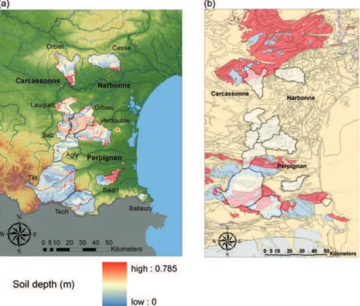
In order to avoid model over-parameterization, the number of parameters to estimate via calibration was kept as low as possible. Spatial patterns of sev-eral parameters were derived from soil surveys and a unique correction coefficient was then applied to each parameter map. This approach was chosen for three parameters, namely the distributed saturated Fig. 3 (a) Soil depth map (source: BD-sols Languedoc Roussillon, INRA), (b) simplified geological formations (red = metamorphic, blue = plutonic, yellow = sedimentary, purple = volcanic, grey = no data) and faults (source: BD Million-Géol, BRGM).
Table 2 Main components of catchment bedrock, referring toFig. 3, right.
Catchments Geology
Tech, Têt - Granite and/or Primary era formations (mainly schist but locally highly karstified limestone) Verdouble, Agly,
Ballaury
- Granite and/or Primary era formations, (top right Verdouble and bottom left Agly on the map) - Mesozoic mainly cretaceous formations (limestone, marl)
Salz, Lauquet, Orbieu
- Primary era formations
- Mesozoic, mainly cretaceous formations,
- Tertiary era detritic formations (sand, molasses, conglomerate) - Quaternary alluvia
Cesse, Orbiel, Réart - Granite and/or Primary era formations (mainly schist but locally highly karstified limestone) - Tertiary era detritic formations (sand, molasses,conglomerate)
hydraulic conductivity K, the lateral transmissivity T0
and soil thickness Z. The calibration procedure con-sists of estimating three coefficients of correction, one for saturated hydraulic conductivity, named CK,
a second for lateral subsurface flow transmissivity, CKSS, and the third for soil thickness, CZ. The
Strickler roughness of the main channel KD1 and
the Strickler roughness of the overbank of the drai-nage network KD2 are also calibrated. The choice of
these parameters follows observations made during a calibration process in the Mediterranean region (Roux et al.2011). Concerning the subsurface lateral transmissivity KSS, the spatial variability is taken
from the vertical hydraulic conductivity map, and the correction coefficient ranges from 100 to 10 000 as horizontal flows are considered faster than vertical ones (see Maidment 1992). Calibration parameters
and variation range are reported in Table 3. In prac-tice, initial ranges of parameter values for Monte Carlo sampling are chosen with the intention of exploring a large range of model behaviours. Uniform parameter distributions within their range of variation are mainly used in the absence of prior information.
4 EVENT MODEL SENSITIVITY ANALYSIS 4.1 Objective of the sensitivity analysis
The aim of this section is to analyse the main char-acteristics of MARINE model response via a compar-ison based on the entire dataset for each flood event and for each catchment. The sensitivity analysis of the MARINE model to the five parameters presented Fig. 4 MARINE model structure, parameters and variables. Green and Ampt infiltration equation: i: infiltration rate (m s-1); I: cumulative infiltration (mm); K: saturated hydraulic conductivity (m s-1); ψ: soil suction at wetting front (m); θsand θi:
saturated and initial water contents, respectively (m3m-3). Subsurface flow: T0: local transmissivity of fully saturated soil
(m2s-1); θsand θ: saturated and local water contents, respectively (m3m-3); m: transmissivity decay parameter (-); β: local
slope angle (rad). Kinematic wave: h: water depth (m); t: time (s); u: overland flow velocity (m s-1); x: space variable (m); r: rainfall rate (m s-1); i: infiltration rate (m s-1); S: bed slope (m m-1); and n: Manning roughness coefficient (m-1/3s).
Table 3 Parameter description and variation range for Monte Carlo analysis.
Description Min Max
Ck Correction coefficient of the hydraulic conductivity (-) 0.1 10 CZ Correction coefficient of the soil thickness (-) 0.1 10 CKSSs Correction coefficient of the soil lateral transmissivity (-) 100 10000 KD1 Strickler roughness coefficient of main channel (m1/3s-1) 1 40 KD2 Strickler roughness coefficient of the overbank (m1/3s-1) 1 30
above is performed for various hydrological responses within a catchment, and across various physiographic conditions within our catchment data-set. The whole parameter space defined inTable 3is explored for different physical behaviours. Moreover, different rainfall products are used for several flood events. For each of them, water conservation controls and simulated runoff coefficients are explored using the sensitivity analysis results and particularly the cumulative distribution function of the parameter CZ, which is the main control on water balance. As
previously mentioned, the aim of the sensitivity ana-lysis is to prepare for the calibration of catchment parameter sets and reduce the significant uncertainty introduced by rainfall QPE data in flash flood modelling.
The global sensitivity analysis method with cost function considering features characterizing the flood peaks is presented. The impacts of the cost function and the threshold choice on the uncertainty interval and best simulations are shown. Monte Carlo simula-tions with several rainfall products are presented, with a discussion on water balance modelling. Catchment sensitivity averaged over flood events is then calculated. The most sensitive parameter of the MARINE model on average, CZ, is studied through
its posterior distribution functions (pdfs) for each catchment and flood. With respect to this parameter, mean catchment behaviour can be found, enabling comparison and selection of QPE for a flood given the identified catchment behaviour.
4.2 Sensitivity analysis method: GSA-GLUE The generalized sensitivity analysis is performed fol-lowing the method proposed by Hornberger and Spear (1981). For each flood event (and each rainfall product for a given flood) the sensitivity analysis is performed, based on a 5000-member Monte Carlo sample obtained with a standard random generator. The MARINE model is run with these 5000 para-meter sets. Each set of parapara-meter values is then assigned a likelihood of being a simulator of the system, on the basis of the chosen likelihood mea-sure. All model realizations are weighted and ranked on this likelihood scale. On the basis of this like-lihood measure, a classification is applied to the model output, resulting in a classification of each model run as behavioural or non-behavioural. The threshold for differentiating between the two classes is a chosen value of the likelihood measure. The cost
function and the threshold are determined subjec-tively, as discussed by Freer et al. (1996).
The separation between the prior and posterior marginal cumulative distributions is subsequently used as a sensitivity measure (Hornberger and Spear 1981): for each parameter αk, the distributions
rela-tive to behavioural and non-behavioural simulations are plotted. A separation between these distributions indicates that the parameter is important for simulat-ing the behaviour studied. The contrary is not always true. Indeed the distributions may show no separation whereas the parameter αkcan be crucial for the
simu-lation because of corresimu-lations with other parameters. It is a necessary but not sufficient condition that parameters must be sensitive to be identifiable. Moreover, sample size and sampling variability should be increased systematically to ensure conver-gence and robustness of the confidence interval respectively.
In the GLUE approach, the likelihood weights associated with the behavioural simulations are applied to their respective model discharges at each time step to give a cumulative distribution of dis-charges at each time step. Uncertainty quantiles can be calculated from these distributions to represent model uncertainty (Freer et al.1996).
4.3 Cost function and threshold value
The highly nonlinear mathematical formulation of rainfall–runoff transformation produces complex response surfaces for hydrological models. The first step of a sensitivity analysis consists of defining a method that evaluates how well the model conforms to the observed behaviour. But, there is no consensus defining a unique criterion to assess model perfor-mance and different objective functions can lead to identification of different parameter combinations (Zin 2002). Besides, we can distinguish methods that use either a partitioning or complete rainfall– runoff records, such as multi-objective optimization (Vrugt et al.2003). Wagener et al. (2003) propose the concept of dynamic identification with moving win-dows and, more recently, Choi and Beven (2007) proposed working on sub-periods characterized by similar hydrological behaviour.
This study is focused on a dataset composed of contrasting catchment flood responses (Garambois et al. 2014). The advantages of including several criteria for model performance evaluation, especially for flood modelling, have been pointed out (Aronica et al.1998,2002, Werner 2004). The cost function,
LNP, introduced by Roux et al. (2011) is used, which,
in addition to the classical normalized least squares approach, considers features characterizing the flood peak (discharge value and time to peak) (Lee and Singh 1998): LNP¼ 1 3"Nash þ 1 3" 1 $ Qp s $Qpo ! ! ! ! Qpo " # þ1 3" 1 $ Tp s $Top ! ! ! ! Tc o " # (1)
where QPsand QPoare respectively the simulated and
observed peak runoff, TPs and TPo are respectively
the simulated and observed time to peak, and Tco is
the time of concentration of the catchment, with
Nash ¼ 1 $ P Nobs i¼1 Qt s$Qto % &2 P Nobs i¼1 Qt o$Qo % &2 (2)
where Nobsis the number of observation data, and Qs
and Qo are respectively the simulated and the
observed runoff. The time of concentration of the catchment is ‘defined using the Bransby formula:
Toc¼ 21:3L A0:1S0:2
(3) where L is the channel length (m), A is the watershed area (m2) and S is the slope of the linear profile. Discharge data are available at 1-h intervals before 2005 and at 5-min intervals thereafter.
Compared to the Nash criterion (equation (2)) the LNPcost function grants more importance to peak
flow value and timing, which is particularly appro-priate for the MARINE model, as it focuses more on flash flood peak flow modelling than on baseflow or recession. It is shown to be the correct compromise for exploring a range of catchment flood behaviours, since it enables simulations to be selected that can be of great use in flood forecasting. The best simulations are shown below.
As explained above, for each flood event and rainfall product, confidence intervals and parameter posterior distribution functions are calculated with the GSA-GLUE method. The influence of the thresh-old is visible in Fig. 5; a higher value gives a nar-rower uncertainty interval and a smaller number of behavioural simulations. Moreover, the added value
of LNP, with respect to the classical Nash, is shown
for this major flood event on the Orbieu: relative error on peak discharge is lower for the best simula-tions (Fig. 5).
The threshold chosen on LNP for this method
is 0.7 in order to have a sufficient number of behavioural simulations on contrasting catch-ments. This choice appears reasonable since it ensures (on average 500 behavioural simulations out of 5000 parameter sets) that the number of behavioural simulations ranges from 300 to nearly 1000 for the best-simulated events. For some floods the best simulations can result in LNP
greater than 0.95. This threshold is relatively high for the LNP function in flash floods, as
attested by the narrow uncertainty interval (Fig. 6). The observations fall within this interval for most of the flood hydrograph. Moreover the uncertainty, especially for peak flow, is below 40%, which is similar to the high flow gauging uncertainty for some catchments and thus the limit of acceptability as defined by Blazkova and Beven (2009). We focus on peak dynamics, according to our cost function, and so it is not surprising if the confidence interval does not fit the observed discharges for the early rising limb or during recession (Fig. 6(a)). It should be remembered that neither baseflow nor recession curves are used in the MARINE model.
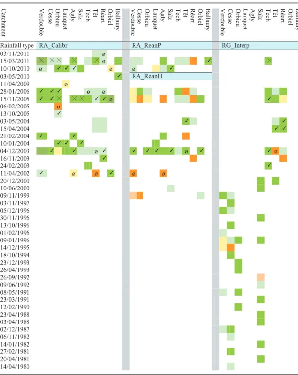
4.4 Event analysis with several rainfall products Monte Carlo simulations were performed for each catchment with different rainfall products for some events, when available. A colour scale is applied (Table 4) in order to help visual qualification of performance for event calibration with the different rainfall products (Table 5). Dark green is for the best Monte Carlo simulations for which GSA-GLUE is possible with respect to the hypothesis presented before. We can observe that Monte Carlo simulations give good results for all the catchments considered. Indeed, for each catchment, the four rainfall products give at least one flood with the best mark, i.e. (Nash, LNP) > 0.8 and two above,
(Nash, LNP) > 0.7. All the rainfall products can
therefore be considered suitable for flash flood mod-elling purposes on these 11 Mediterranean catchments.
Radar rainfall data seem to improve the possibi-lity of flood modelling, since many of the floods simulated with RA_Calibr give satisfactory
performances, with (Nash, LNP) > 0.7. The two that
do not give correct results for RA_Calibr are very low flow events (6 February 2005 for the Orbieu and 10 April 2002 for the Têt), which seems reasonable, as MARINE was originally developed to simulate extreme events. Interpolated raingauges from the
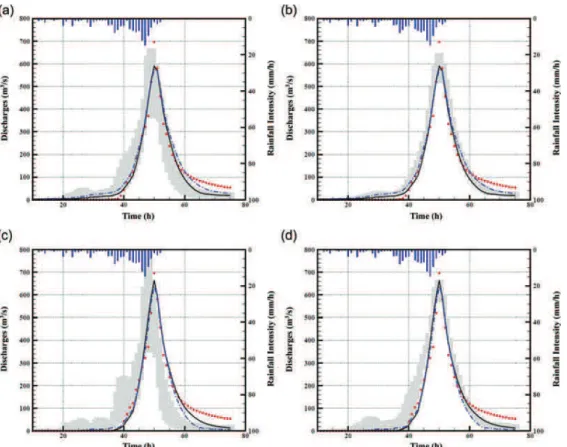
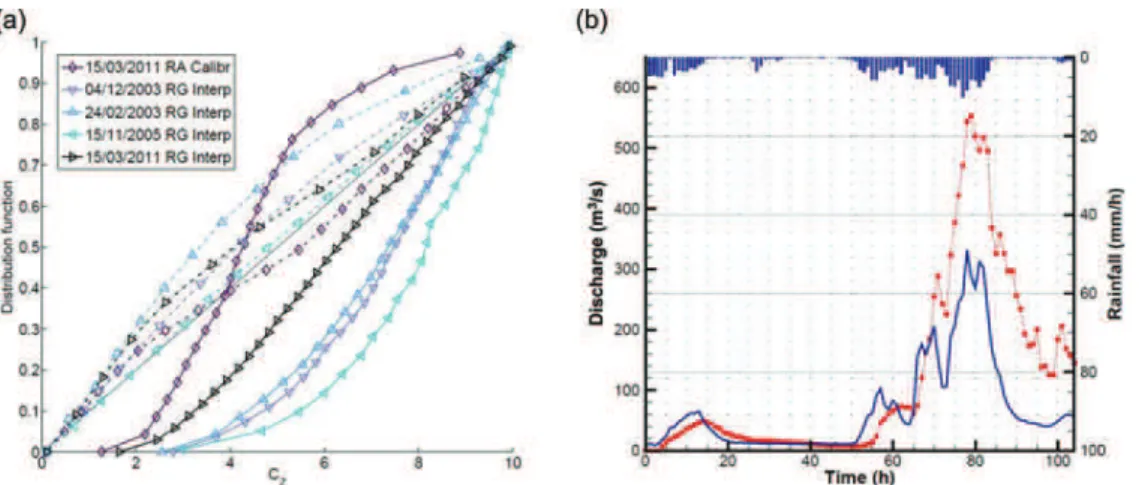
dense measurement network give good results (Table 5). It should be noted that even a dense cover-age with five raingauges for the Verdouble catchment (299 km2) did not provide good modelling results for the 8 January 1996 and 14 December 1995 events. The rainfall measurement network may not have seen Fig. 6 Observed discharge (dots), two best simulations (solid and dashed lines) and confidence interval for: (a) the Orbieu at Lagrasse (263 km2) 15 November 2005 flood event, performed with RA_Calibr radar rainfall data, LNPthreshold = 0.7,
900 behavioural simulations; (b) the Tech at Pas-du-Loup (250 km2), 15 November 2005 flood event, performed with RG_Interp interpolated rainfall data from five raingauges, LNPthreshold = 0.7, 480 behavioural simulations.
Fig. 5 Observed discharge (dots), best simulations (solid and dashed lines) and uncertainty interval (5–95% quantiles) for the Orbieu at Lagrasse (263 km2), 15 November 2005 flood event performed with RA_Calibr radar rainfall data: (a) Nash threshold = 0.5; (b) Nash threshold = 0.9; (c) LNPthreshold = 0.5; (d) LNPthreshold = 0.9.
Table 4 Efficiency intervals and colour correspondence.
Performance condition for the couple (Nash, LNP) > 0.8 > 0.7 > 0.65 > 0.5 < 0.5
Colour correspondence
Table 5 Event calibration efficiencies. Not all the cells are filled, as a storm-flood event can concern several catchments without affecting the whole dataset. Rainfall products selected with the CZ pdf
similarity method for each catchment since 2002 for calibration (✓), products selected but not used for calibration (%), Ø is for flood events where no rainfall product is chosen.
part of rainfall explaining catchment response for these two events.
Simulations in yellow or orange (Table 5), mostly for interpolated raingauges (RG_Interp) or RA_ReanH, are simulations that do not reproduce the observed hydrograph correctly. A low value of LNP often corresponds with simulations with
under-estimated peak flow, but still good temporal dynamics and simulated peak time. That is to say for the simulation marked in yellow and orange, the model water balance is not able to reproduce the order of magnitude of peak discharge, and conse-quently the flood water balance.
Most floods and catchments are correctly mod-elled with MARINE. Although parameter sets are sampled in relatively wide ranges in order to be able to reproduce different catchment behaviour for several events, all 5000 simulations result in signifi-cant underestimates of peak flow. This addresses the question of which phenomenon leads to such an error in water conservation modelling.
In our modelling of rainfall-to-runoff conserva-tion, the four most important sources of error are probably:
(a) QPE under- or over-estimates; (b) High-flow gauging errors;
(c) model structure and parametric compensation (bedrock loss and evapotranspiration not simulated);
(d) initial soil moisture estimates.
First, the sources of uncertainty (b)–(d) are con-stant for a given event, so, when considered with different rainfall products, comparisons are possi-ble. We are conscious of problems relating to rat-ing curve quality and initialization errors, but this is not the purpose of this study and it may have a limited impact on the results under our hypothesis. Indeed, most events are of comparable order of magnitude for a given catchment, so we can neglect gauging errors between events. The initia-lization error inherent in event models is not taken into account since in the MARINE model soil saturation is fixed by the root zone moisture, simu-lated by the continuous water balance model SIM (Habets et al. 2008) at the beginning of each flood event. The initial soil moisture for the 43 flood events dataset is on average 57.7% with a rather low standard deviation of 6.6%, so from this varia-tion range its impact on MARINE sensitivity is considered limited.
4.5 Catchment sensitivity to parameters
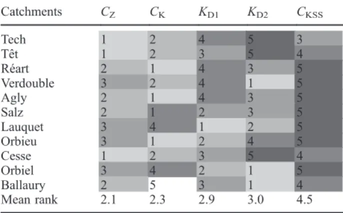
Monte Carlo simulations for each catchment are per-formed under identical mathematical and physical hypotheses and with the same data types, in order to be able to compare MARINE results and sensitiv-ity between events and catchments. Table 6 shows mean parameter rank for each catchment, obtained by averaging Kolmogorov-Smirnov test values for all the events considered for GSA-GLUE analysis per catchment, with selected rainfalls (Table 7). Mean parameter rank (and thus model sensitivity to flow components) varies as a function of the catchment; CZ, the spatial soil multiplicative constant, is the
most sensitive parameter on average followed by CK, whereas CKSS, lateral soil transmissivity, is the
least sensitive. No clear tendency appears for KD1
whose sensitivity depends mainly on catchment prop-erties. No clear trend appears for the overbank rough-ness KD2 either, whose rank can vary from 1 to 5,
with an average of 3.
On average, MARINE evaluated with the LNP
cost function is mostly sensitive to CZ and CK,
defining catchment storage capacity and infiltrabil-ity. These two sensitive parameters thus indicate that MARINE is mainly sensitive to runoff production dynamics and amounts for flash flood events. The sensitivity of the channel transfer function, repre-sented by main channel roughness and floodplain roughness, is also considerable, whereas subsurface transfer is less sensitive according to the model. Low interactions were found between parameters through covariance analysis with global sensitivity analysis.
Table 6 Mean catchment parameter ranking according to Dmax calculated for each parameter and event, Dmax being the maximum separation between the behavioural and non-behavioural distributions. Mean parameter rank is obtained by averaging each parameter rank for all the catchments. Catchments CZ CK KD1 KD2 CKSS Tech 1 2 4 5 3 Têt 1 2 3 5 4 Réart 2 1 4 3 5 Verdouble 3 2 4 1 5 Agly 2 1 4 3 5 Salz 2 1 2 3 5 Lauquet 3 4 1 2 5 Orbieu 3 1 2 4 5 Cesse 1 2 3 5 4 Orbiel 3 4 2 1 5 Ballaury 2 5 3 1 4 Mean rank 2.1 2.3 2.9 3.0 4.5
4.6 Sensitivity to spatial soil depth and water volume control
In this section we focus on the spatial soil depth multi-plicative constant, CZ, which, on average, is seen to be
one of the most sensitive parameters of the MARINE model for the 11 catchments. Indeed, CZis responsible
for catchment storage capacity and water balance adjustments: it controls a catchment’s soil volume and can compensate runoff volume in a non-negligible but still physical range (CZ∈ [0.1, 10]). Roux et al.
(2011) previously showed the sensitivity of MARINE to CZ on the Gardon d’Anduze
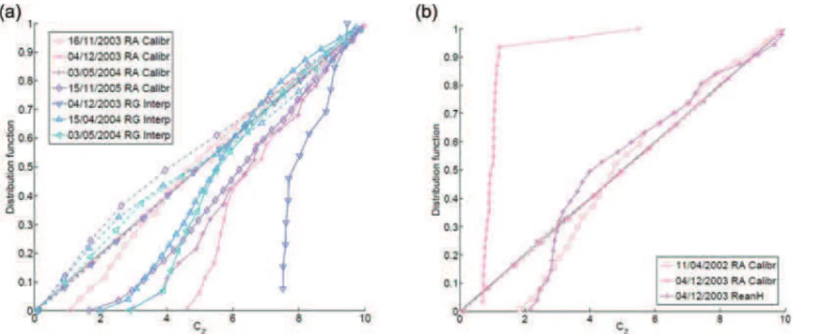
catch-ment in the Cévennes; this parameter is found to explain 80% of model output variance when hydro-graphs peak on several Mediterranean catchments (Garambois et al. 2013). Le Lay and Saulnier (2007) with TOPMODEL, and Braud et al. (2010) with CVN and MARINE models showed that soil depth strongly influences the flash flood response of catchments in the Cévennes. After applying the MARINE model to 11 Mediterranean catchments, we present CZ posterior distribution
functions (pdfs) (Figs 7–12). Several events are plotted on one graph in order to compare the pdf shapes, each pdf coming from one Monte Carlo sample. The following interpretations are based
on the results of the sensitivity analysis (posterior distribution functions Figs 7–12 summarized in the parameter ranking of Table 6).
According to the Kolmogorov-Smirnov tests performed above, CZ is the most sensitive parameter
for Tech, Têt and Cesse compared to the eight other catchments (Table 6). Concerning Tech and Têt, the shape of the pdfs shows that most of the behavioural simulations are for CZ values greater than 4,
espe-cially for the Têt (CZ> 5,Fig. 7(b)). Sensitivities are
similar for these two catchments, which are mainly located on metamorphic terrain.
The Cesse (Fig. 8(a)), Ballaury (Fig. 8(b)), Réart (Fig. 9(a)), Agly (Fig. 10(b)) and Salz (Fig. 12) catchments are also very sensitive to CZ, and most
of the behavioural simulations are for CZ values of
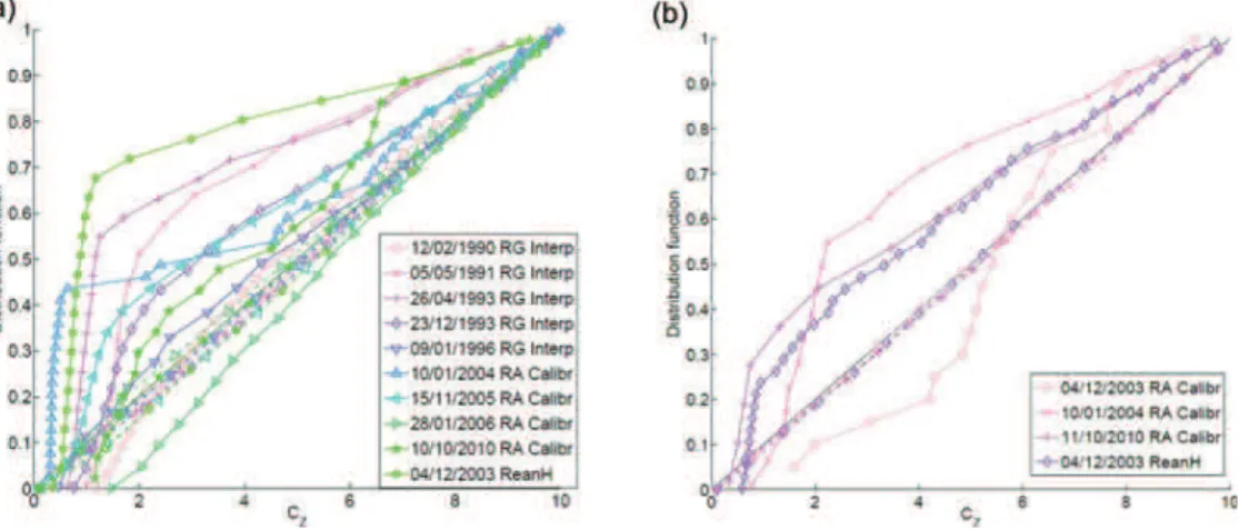
between 1 and 4. The physiographic and bedrock properties are complex for these catchments: Cesse is highly karstified (Nou et al.2011) and Réart pre-sents mixed and complex physiographic properties. The Verdouble (Fig. 10(a)), Lauquet (Fig. 11(b)) and Orbieu (Fig. 11(a)) catchments from the Corbières Hills, and the Orbiel catchment (Fig. 9(b)) from the Montagne Noire are less sensitive to CZ than the
previous catchments, and overall most of the beha-vioural simulations are for values of CZ > 1. The
substrates of these basins were mainly developed from sedimentary bedrock (Table 2) overlain by loam and silty loam.
Bedrock loss is not represented in the model. This might be responsible for CZ values greater
than one, as suggested by Castaings et al. (2009) and Roux et al. (2011). The modeller therefore needs to increase soil volume and thus storage capa-city, to produce a correct runoff volume for hydro-graph formation given a QPE. Bedrock type and alteration might explain the large differences between catchment sensitivity and parameterization for CZ.
4.7 Selection of rainfall QPE with the sensitivity analysis method and mean catchment behaviour
For each catchment, most of the flood events recorded and simulated with Monte Carlo sampling are eligible for GSA-GLUE (Table 5), (Nash, LNP > 0.8). In other words, it is possible to find
parameter sets producing good performances for one or more rainfall inputs. The final objective is to find correct sets of events/rainfalls for gauged catch-ment calibration, in order to be able to calibrate the Table 7 Calibrated catchment parameter sets, Nash cost
function. Global Nash is the cost function for the whole calibration set, min Ev Nash corresponds to single-event Nash and max EV Nash to single-event maximum Nash for each part of the multiple events hydrograph. Simulated and observed runoff coefficients and efficiencies for vali-dation events.
Catchment Salz Tech Verdouble Calibration: CZ 0.95 4.34 1.3 CK 20 11 15 CKSS 5595 1515 4486 KD1 5 4.83 5 KD2 2.54 3.24 3.99 Global Nash 0.89 0.9 0.88 min Ev Nash 0.61 0.89 0.74 max Ev Nash 0.9 0.91 0.95 Validation: Event 20/12/2000 15/03/2011 15/03/2011 Observed runoff coefficient 0.45 0.61 0.55 Simulated runoff coefficient 0.62 0.42 0.63 Nash 0.61 0.69 0.89 LNP 0.7 0.74 0.87
Fig. 8 Event posterior distribution functions: (a) Cesse at Bize-Minervois, and (b) Ballaury at Banyuls (solid line: beha-vioural simulations, dash-dot line: non-behabeha-vioural simulations).
Fig. 9 Event posterior distribution functions: (a) Réart at Salleilles, and (b) Orbiel at Villedubert (solid line: behavioural simulations, dash-dot line: non-behavioural simulations).
Fig. 7 Event posterior distribution functions: (a) Tech at Pas du Loup, and (b) Têt at Marquixane (solid line: behavioural simulations, dash-dot line: non-behavioural simulations).
model. The results of the sensitivity analysis show that, on each catchment, the different events can present different shapes of posterior distribution func-tions for the same parameter, namely CZ. The
meth-odology of event selection starts from the consideration that events with similar sensitivity to CZ are likely to present similar averaged behaviours
in terms of rainfall-to-runoff volume conservation. We therefore take into consideration the rainfall input leading to the a posteriori CZ pdf closest to
those of other events, i.e. producing comparable mean behaviour. Strong or extreme events regarding their peak flow are not used for SA and calibration but rather kept for validation. The procedure to select one rainfall product uses event sensitivity analysis (SA) with radar rainfall records (RA_Calibr) by default, other rainfall products (radar RA_ReanH, RA_ReanP or raingauges RG_Interp) are then Fig. 11 Event posterior distribution functions: (a) Orbieu at Lagrasse, and (b) Lauquet at St Hilaire (solid line: behavioural simulations, dash-dot line: non-behavioural simulations).
Fig. 12 Event posterior distribution functions, Salz at Cassaignes (solid line: behavioural simulations, dash-dot line: non-behavioural simulations).
Fig. 10 Event posterior distribution functions: (a) Verdouble at Tautavel, and (b) Agly at St Paul de Fenouillet, (solid line: behavioural simulations, dash-dot line: non-behavioural simulations).
considered if: (a) there are not enough behavioural simulations with RA_Calibr to perform a GSA-GLUE analysis, and (b) one event presents a very dissimilar a posteriori CZ pdf with respect to the
other events. Indeed, for a given catchment, large dissimilarities between events for CZ sensitivity and
unusual CZ values identified can be attributable to
QPE errors under our hypothesis. While keeping such events for the calibration phase, we examine the other pdfs obtained from different rainfall types, if available for an event. However, all the events considered are not systematically simulated with all rainfall products, because of availability issues, for example.
Several rainfall products were selected with this method, especially in cases where unusual catchment behaviour were detected, for example:
– On the Tech catchment (Fig. 7(a)), pdfs from RA_Calibr show different sensitivities and result-ing CZ values, whereas pdfs from RG_Interp
show similar behaviour for the events of 24 February 2003, 4 April 2003 and 15 November 2005: the RG_Interp rainfall product of these three events was chosen for calibration.
– On the Têt catchment (Fig. 7(b)), for the events of 15 April 2004, 2 May 2004 and 28 January 2006, RG_Interp and RA_ReanH products were chosen as presenting similar behaviour.
Interpolated raingauge data (RG_Interp) can give good results in terms of Nash and LNP and for pdf
similarity in several cases. This may be attributable to raingauge density and locations that seem to capture enough rainfall variability for satisfactory flood mod-elling. The case of the event of 4 December 2003 on several catchments particularly highlights the pro-blem. Different rainfall products were chosen for this event, according to the location of the considered catchment. On the Cesse (Fig. 8(a)) and the Agly (Fig. 10(b)), pdfs from RA_Calibr are consistent with pdfs of other events on the same catchment. On the Tech (Fig. 7(a)), RG_Interp gave pdfs with the greatest similarity to other events, while on the Salz (Fig. 12), the Lauquet (Fig. 11(b)) and the Orbiel (Fig. 9(b)), RA_ReanH provided the most similar pdfs. It seems that depending on the location of the catchment with respect to the radar, rainfall variability is not always well captured by the same rainfall product. As already mentioned, for the Tech and Têt catchments, raingauges give better results than radar data, maybe because they are the catch-ments at the greatest distance from the radar. In
addition, high-relief topography with deep narrow valleys may disturb radar measurements.
However, pdf similarity does not exclude various hydrological behaviours for a particular catchment. For example, both small events and strong events that certainly activate different flow paths and runoff for-mation dynamics within a catchment, can present similar pdfs, as for 15 November 2005 for the Verdouble (3.3 m3 s-1 km-2) and the Orbieu (2.65 m3 s-1 km-2) or 2 December 1987 for the Cesse (2 m3 s-1 km-2). This is true for catchments that are both sensitive and less sensitive to CZ. As a
result we do not exclude various catchment beha-viours that can be caused by different rainfall spa-tio-temporal variability.
The method enabled us to select a rainfall pro-duct on almost all the catchments (Table 5). However the selection was particularly difficult on the Orbieu catchment for which it seems impossible to identify a mean behaviour (Fig. 11(a)). Altogether, the selection has been more difficult for the catchments for which the behavioural simulations were for CZ close to 1
and easier for catchments for which the behavioural simulations were for greater CZ values.
Different sensitivity and calibrated values of the CZcoefficient between catchments can indicate
differ-ent rainfall-to-runoff volume conservation relations for catchments. The pdf analysis is applicable to different rainfall types such as radar or interpolated raingauge data, as results can attest. It seems that Opoul radar rainfall data quality is quite variable in time and space with QPE errors sometimes significantly affecting hydrological modelling sensitivity and performance. 5 CALIBRATION OF CATCHMENT
PARAMETER SETS WITH SELECTED RAINFALL EVENTS
To perform real time predictions and regionalization, one parameter set per catchment may be required. The objective of this section is two-fold: to document the difficult problem of calibration for flash-flood event models with results performed for three med-ium-sized catchments, Salz, Tech and Verdouble (144–299 km2), areas located on contrasting bed-rocks, and showing the benefit of selecting the right rainfall dataset. Several events and rainfall data types were selected with the SA method presented above.
Here, we use an optimization technique over several calibration flood events considered together. Calibration is performed using a BFGS minimization algorithm (Broyden-Fletcher-Goldfarb-Shanno) called
M2QN1 (Lemaréchal and Panier2000) with a sum of square error (SSE) cost function. The five sensitive parameters of the MARINE model are calibrated for five random starting points in the parameter ranges (Table 6). This multiple direction optimization algo-rithm is used both for calibration and real time varia-tional data assimilation within the MARINE model (Castaings et al. 2009). The LNP would be suitable
for a multi-objective calibration, but its implementa-tion requires addiimplementa-tional observaimplementa-tion data. The aim here is not to discuss the calibration method, which often converges on the same parameter combination from different starting points in the parameter space, but to illustrate the usefulness of pdf selection for rainfall analysis.
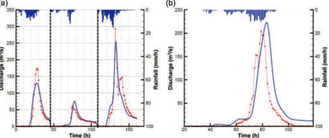
The calibration leads to satisfactory Global Nash efficiencies of around 0.9 for complete sets (Table 7), and peak simulation errors below 30%, which is reasonable in the case of flash floods (Figs 13–15). Validations are presented on one event for each catchment, and (Nash, LNP) efficiencies range from
(0.61, 0.7) for Salz to (0.89, 0.87) for Verdouble (Table 7). It should be noted that validation efficien-cies are fairly close to calibration efficienefficien-cies.
The example of the 15 March 2011 event on the Tech illustrates the benefits of this method. Indeed the CZpdf of this 15 March 2011 (RA_Calibr) event
on the Tech was not similar to the other pdfs and suggested that QPE was underestimated, as con-firmed by validation (Fig. 16) and the runoff coeffi-cient (Table 7). Single calibration for this event give CZ values around 2.5. In validation with the
cali-brated parameter set of Table 7, peak flow is under-estimated by about 40% (Fig. 16, right). Considering (RG_Interp) rainfalls, the peak flow underestimation is smaller, at about 15% (Fig. 14).
A larger CZ parametric compensation
(CZ = 4.34) is required for the Tech catchment,
while the two other catchments need CZ ≈ 1
(Table 7). Initial and maximal soil saturations are comparable for the three catchments and the soil data (pedology) from the BD-sol give a mean soil thickness of 0.31 and 0.33 m for the Salz and Verdouble, respectively, and 0.16 m for the Tech (Table 1). So catchment storage capacity has to be increased by a factor of 2 or more for the granite and primary era altered substrates, as for the Tech or Têt catchments.
The calibration procedure leads to relatively low main channel KD1and overbank KD2roughness, i.e.
significant friction is necessary to delay the flow. This might be due to water partition, with a surplus
drained quickly with surface runoff on hillslopes and in the drainage network. Subsurface lateral transfer tends to be slower. This indicates that water distribu-tion between lateral flow components and other mechanisms, such as exfiltration in the drainage net-work, and its representation need to be improved. Measurements at different scales are still necessary to better constrain these flow dynamics.
Maps of maximum soil moisture deficit are plotted for Tech and Verdouble validation events (Fig. 17). Nearly the whole Verdouble catchment is saturated at 10 h, just before peak time, whereas, for the Tech, several areas close to the main drain and the middle of the catchment have a minimum deficit of 27%. Peak flow underestimation on the Tech catch-ment might be explained by underdevelopcatch-ment of contributing areas mainly because of rainfall under-estimation and location errors (Fig. 14(b)). The pos-sibility of mapping state variables (Fig. 17) is interesting to compare, for example, the development of the extent of contributing areas for typical soil configurations.
6 CONCLUSION
The 11 catchment headwaters of the eastern Pyrenees foothills, with areas ranging from 36 to 776 km2, are interesting study sites for flash-flood generating mechanisms, given the quantity of static, meteorolo-gical and hydrometric data available. They present contrasting physical properties and behaviours that can be detected with the help of statistics (Garambois et al.2011).
Global sensitivity analysis of the MARINE model is performed on each event for a catchment given various flood responses. MARINE model for-mulation was found to be an appropriate tool for flash-flood modelling with various rainfall data types, even for small catchments, as the number of event simulations eligible for GSA-GLUE can attest. Global mean behaviours are identified for each catch-ment and differences between catchcatch-ment sensitivity and parameterization for the water balance parameter CZ can be attributed to deep percolation in altered
bedrock, as suggested by other authors (Castaings et al. 2009, Roux et al. 2011). Indeed, catchments needing a larger CZ value present substrates that
develop on granite, schist and primary era formations and that seem to present the highest bedrock storage as shown by Vannier et al. (2014) with recession analysis in the Cévennes-Vivarais region. This may be due to the fact that the soil depth used in
Fig. 15 Verdouble catchment (299 km2): (a) calibration (blue solid line) and observed discharge (red dotted line) over four different flood events, 11 April 2002 (RA_Calibr), 15 November 2005 (RA_Calibr), 28 January 2006 (RA_Calibr), 10 October 2010 (RA_Calibr); and (b) parameter set validation for 15 March 2011 (RA_ReanP).
Fig. 13 Salz catchment (144 km2): (a) calibration (blue solid line) and observed discharge (red dotted line) over three different flood events, 4 December 2003 (RA_ReanH), 10 January 2004 (RA_Calibr), 11 October 2010 (RA_Calibr); and (b) parameter set validation for 23 December 2000 (RG_Interp).
Fig. 14 Tech catchment (250 km2): (a) calibration (blue solid line) and observed discharge (red dotted line) over three different flood events, 24 February 2003 (RG_Interp), 4 December 2003 (RG_Interp), 15 November 2005 (RG_Interp); and (b) parameter set validation for 15 March 2011 (RG_Interp).
modelling only takes soil horizons A (surface soil) and B (subsoil) into account. Horizons C (parent rock) and R (bedrock) are not taken into account even though they may be hydrologically active.
Moreover, the sensitivity of the soil thickness multiplicative constant controlling the water balance of the MARINE model enables the selection of rain-fall input with respect to an identified catchment behaviour. This method was seen to be useful in this study for rainfall product selection on some catchments, whereas it can be difficult to choose between two rainfall products with a direct compar-ison, as shown in Section 2.1. Among the possible reasons for the fluctuating quality of the data there might be the lumpy topography, the readjustment procedure or the position of the radar, which can cause wet radome situations or other sources of attenuation.
The method proposed here is applicable for any conservative hydrological model with an explicit sto-rage parameter. Model calibration with the selected events was performed using the MARINE model. Multiple event calibration and validation give perfor-mances ranging from 0.7 to 0.89. For model calibra-tion, it is useful to understand how to parameterize soil volume (and thus storage capacity) for several types of substrates/bedrocks. Moreover, good calibra-tion and validacalibra-tion efficiencies with a soil similarity approach are an interesting basis for flash flood pre-diction at ungauged locations with a distributed model. Indeed, this calibration process aims at find-ing a mean physical behaviour through flood water balance for each catchment which can be interesting for transferring parameter sets to ungauged catch-ments with respect to physiographic descriptors of the catchment for example.
Fig. 16 Tech at Pas du Loup: (a) event posterior distribution function, and (b) calibrated parameter set test (blue solid line) and observed discharge (red dotted line) for 15 March 2011 (RA_Calibr).
Fig. 17 Maximum soil saturation for the 15 March 2011 event: (a) Verdouble at Tautavel at 10 h, and (b) Tech at Pas du Loup at 22 h.
Acknowledgements The authors gratefully acknowl-edge data supply by the French central flood fore-casting service, SCHAPI3 and the regional flood forecasting service, SPCMO.
Funding The authors gratefully acknowledge the financial support of the SCHAPI.
REFERENCES
Andréassian, V., et al., 2001. Impact of imperfect rainfall knowledge on the efficiency and the parameters of watershed models. Journal of Hydrology, 250 (1–4), 206–223. doi:10.1016/ S0022-1694(01)00437-1
Aronica, G., Bates, P.D., and Horritt, M.S., 2002. Assessing the uncertainty in distributed model predictions using observed binary pattern information within GLUE. Hydrological Processes, 16 (10), 2001–2016. doi:10.1002/hyp.398
Aronica, G., Hankin, B., and Beven, K., 1998. Uncertainty and equifinality in calibrating distributed roughness coefficients in a flood propagation model with limited data. Advances in Water Resources, 22 (4), 349–365. doi: 10.1016/S0309-1708(98)00017-7
Ayral, P.A., et al., 2007. Forecasting flash floods with an operational model. Advances in Natural and Technological Hazards Research, 25, 335–352.
Bárdossy, A. and Das, T., 2008. Influence of rainfall observation network on model calibration and application. Hydrology and Earth System Sciences, 12, 77–89. doi: 10.5194/hess-12-77-2008
Beven, K., 2006. A manifesto for the equifinality thesis. Journal of Hydrology, 320 (1–2), 18–36. doi:10.1016/j.jhydrol.2005.07.007
Beven, K.J. and Binley, A.M., 1992. The future of distributed mod-els: model calibration and uncertainty prediction. Hydrological Processes, 6, 279–298.
Beven, K.J., 2002. Rainfall–runoff modelling: the Primer. Chichester: John Wiley & Sons, LTD.
Beven, K.J., Smith, P.J., and Freer, J.E., 2008. So just why would a modeller choose to be incoherent? Journal of Hydrology, 354 (1–4), 15–32. doi:10.1016/j.jhydrol.2008.02.007
Blazkova, S. and Beven, K., 2009. A limits of acceptability approach to model evaluation and uncertainty estimation in flood fre-quency estimation by continuous simulation: Skalka catch-ment, Czech Republic. Water Resources Research, 45 (12), W00B16. doi:10.1029/2007WR006726
Blöschl, G., 2005. Rainfall–runoff modelling of ungauged catch-ments. In: M.G. Anderson, ed., Encyclopedia of hydrological sciences. Chichester: John Wiley & Sons, 2061–2080. Borga, M., et al., 2008. Surveying flash floods: gauging the
ungauged extremes. Hydrological Processes, 22 (18), 3883– 3885. doi:10.1002/hyp.7111
Braud, I., et al., 2010. The use of distributed hydrological models for the Gard 2002 flash flood event: analysis of associated hydro-logical processes. Journal of Hydrology, 394 (1–2), 162–181. doi:10.1016/j.jhydrol.2010.03.033
Castaings, W., et al., 2009. Sensitivity analysis and parameter esti-mation for distributed hydrological modeling: potential of variational methods. Hydrology and Earth System Sciences J1 -HESS, 13 (4), 503–517. doi:10.5194/hess-13-503-2009
Choi, H.T. and Beven, K., 2007. Multi-period and multi-criteria model conditioning to reduce prediction uncertainty in an application of TOPMODEL within the GLUE framework.
Journal of Hydrology, 332 (3–4), 316–336. doi:10.1016/j. jhydrol.2006.07.012
Costa, J.E., 1987. Hydraulics and basin morphometry of the largest flash floods in the conterminous United States. Journal of Hydrology, 93 (3–4), 313–338. doi:10.1016/0022-1694(87) 90102-8
Creutin, J.-D. and Borga, M., 2003. Radar hydrology modifies the monitoring of flash-flood hazard. Hydrological Processes, 17 (7), 1453–1456. doi:10.1002/hyp.5122
Davolio, S., Buzzi, A., and Malguzzi, P., 2009. Orographic triggering of long lived convection in three dimensions. Meteorology and Atmospheric Physics, 103 (1–4), 35–44. doi: 10.1007/s00703-008-0332-5
Delrieu, G., et al., 2014. Dependance of radar quantitative precipita-tion estimaprecipita-tion error on the rain intensity in the Cévennes region, France. Hydrological Sciences Journal, special issue: Weather radar and hydrology, 59 (7), 1308–1319. doi:10.1080/ 02626667.2013.827337
Duan, Q., Sorooshian, S., and Gupta, V.K., 1992. Effective and efficient global optimization for conceptual rainfall–runoff models. Water Resources Research, 28 (4), 1015–1031. doi:10.1029/91WR02985
Freer, J., Beven, K.J., and Ambroise, B., 1996. Bayesian estimation of uncertainty in runoff prediction and the value of data: an application of the GLUE approach. Water Resources Research, 32 (7), 2161–2173. doi:10.1029/95WR03723
Gaál, L., et al., 2012. Flood timescales: understanding the interplay of climate and catchment processes through comparative hydrology. Water Resources Research, 48 (4), W04511. doi:10.1029/2011WR011509
Garambois, P.A., et al., 2011. Relations between streamflow indices, rainfall characteristics and catchment physical descriptors for flash flood events. In: R.J. Moore, S.J. Cole and A.J. Illingworth, eds. Weather radar and hydrology. (Proceedings of a symposium held in Exeter, UK, April 2011). Wallingford: International Association of Hydrological Sciences, IAHS Publ. 351, 581–586.
Garambois, P.A., et al., 2013. Characterization of process-oriented hydrologic model behavior with temporal sensitivity analysis for flash floods in Mediterranean catchments. Hydrology and Earth System Sciences, 17, 2305–2322. doi: 10.5194/hess-17-2305-2013
Garambois, P.A., et al., 2014. Analysis of flash flood-triggering rainfall for a process-oriented hydrological model. Atmospheric Research., 137, 14–24. doi:10.1016/j.atmosres. 2013.09.016
Gaume, E., et al., 2004. Hydrological analysis of the river Aude, France, flash flood on 12 and 13 November 1999. Journal of Hydrology, 286 (1–4), 135–154. doi:10.1016/j.jhydrol. 2003.09.015
Georgakakos, K.P., 1992. Advances in forecasting flash floods. Proceedings of the CNAA-AIT Joint seminar on prediction and damage mitigation of meteorologicaly induced Natural disasters, 21–24 May, National Taïwan University, Taipei, 280–293.
Gupta, H., et al., 2003. Reply to comment by K. Beven and P. Young on Bayesian recursive parameter estimation for hydro-logic models. Water Resources Research, 39 (5), 1117. doi:10.1029/2002WR001405
Habets, F., et al., 2008. The SAFRAN-ISBA-MODCOU hydrome-teorological model applied over France. Journal of Geophysical Research, 113, D06113. doi:10.1029/2007JD008548
Hornberger, G.M. and Spear, R.C., 1981. An approach to the pre-liminary analysis of environmental systems. Journal of Environmental Management, 12, 7–18.
3