A distributed parsimonious event-based model for flood forecasting in Mediterranean catchments : efficiency of the model and spatial variability of the parameters

(1)

HAL Id: tel-02286774

https://tel.archives-ouvertes.fr/tel-02286774

Submitted on 13 Sep 2019

HAL is a multi-disciplinary open access

archive for the deposit and dissemination of sci-entific research documents, whether they are pub-lished or not. The documents may come from teaching and research institutions in France or abroad, or from public or private research centers.

L’archive ouverte pluridisciplinaire HAL, est destinée au dépôt et à la diffusion de documents scientifiques de niveau recherche, publiés ou non, émanant des établissements d’enseignement et de recherche français ou étrangers, des laboratoires publics ou privés.

A distributed parsimonious event-based model for flood

forecasting in Mediterranean catchments : eﬀiciency of

the model and spatial variability of the parameters

Quoc Son Nguyen

To cite this version:

Quoc Son Nguyen. A distributed parsimonious event-based model for flood forecasting in Mediter-ranean catchments : eﬀiciency of the model and spatial variability of the parameters. Other. Université Montpellier, 2019. English. �NNT : 2019MONTG019�. �tel-02286774�

(2)

RAPPORT DE GESTION

2015

THÈSE POUR OBTENIR LE GRADE DE DOCTEUR

DE L’UNIVERSITÉ DE MONTPELLIER

En Sciences de l'Eau

École doctorale GAIA

Unité de recherche : Laboratoire Hydrosciences Montpellier

Présentée par Quoc Son NGUYEN

Le 4 juillet 2019

Sous la direction de Dr. Christophe BOUVIER

Devant le jury composé de Sandrine ANQUETIN, Directrice de Recherche CNRS, IGE, Grenoble Hélène ROUX, Maître de Conférences INPT,IMFT, Toulouse

Patrick ARNAUD, Ingénieur de Recherche IRSTEA, Aix en Provence Roger MOUSSA, Directeur de Recherche INRA, LISAH, Montpellier Olivier PAYRASTRE, Ingénieur Divisionnaire TPE, IFSTTAR, Bouguenais Christophe BOUVIER, Directeur de Recherche IRD, HSM, Montpellier

Rapporteure Rapporteure Examinateur

Examinateur, Président du jury Examinateur

Directeur de thèse

Application du modèle distribué événementiel SCS -LR

pour la prévision des crues méditerranéennes :

performances du modèle et variabilité spatiale des

(3)

i

Acknowledgments

I would like to express my sincere appreciation and thanks to my supervisor Dr. Christophe Bouvier for the continuous support of my study. I would like to thank you for encouraging my research and for allowing me to grow as a research scientist. Your advice on both research as well as on my career have been invaluable.

I would like to thank the rest of my thesis committee: Dr. Roger Moussa, Dr. Ludovic Oudin, Dr. Lea Garandeau and Dr. Patrick Arnaud for their insightful comments and for the question which incented me to widen my research from various perspectives. I would also be thankful to Dr. Sandrine Anquetin, Dr. Hélène Roux, Dr. Roger Moussa, Dr. Patrick Arnaud, and Dr. Olivier Payrastre to accept to be in my jury.

I am also grateful for the Vietnam International Education Development, University of Science and Technology of Hanoi, Campus France, and SCHAPI for providing the financial support to stay in France and pursue this Ph.D. study.

I would especially like to thank the University Montpellier and HSM and IRSTEA to provide all the supports in terms of workspace, computers, data and facilitating all the paper works that allow my researches, as well as my stay in France.

I am also thankful to Dr. Valérie Borrell Estupina for giving me the opportunity to come to France and pursuing my studies in Hydrology, as well as giving me valuable support during my first day here.

I am also thankful for my fellow labmates: Aubin Allies, Camille Jourdan and others for the stimulating discussions, for all the help and all the fun we have had in the last three years; to Madame Catherine Marchand to help me with the administration. Also, I thank all my Vietnamese friends in Marseille and Montpellier for all the supports in life.

Last but not least, I would like to thank my family: my parents, my brother, my beloved wife and my expected daughter for supporting me spiritually throughout writing this thesis and my life in general.

(4)

(5)

iii

Résumé

Les modèles pluie-débit sont des outils essentiels pour de nombreuses applications hydrologiques, notamment la prévision des crues. L’objet de cette thèse est d’examiner les performances d’un modèle événementiel distribué, dont l’intérêt est de résumer la représentation des processus à la phase de crue, et la condition initiale à un indice de saturation du bassin facilement observable ou accessible. Ce dernier dispense de modéliser la phase inter-crue, et simplifie la paramétrisation et le calage du modèle. Le modèle étudié combine une fonction de production type SCS et une fonction de transfert type lag and route, appliquées à une discrétisation du bassin en mailles carrées régulières.

Le modèle est d’abord testé sur le bassin versant du Real Collobrier. Ce bassin méditerranéen est suivi depuis plus de 50 ans par l’IRSTEA, et dispose d’une exceptionnelle densité de mesures de pluies et de débits. Cet environnement favorable permet de limiter les incertitudes sur l’estimation des pluies et d’évaluer les performances intrinsèques du modèle. Dans ces conditions, les crues sont bien reconstituées à l’aide d’un jeu de paramètres unique pour l’ensemble des épisodes testés, à l’exception de la condition initiale du modèle. Celle-ci apparaît fortement corrélée avec l’humidité du sol en début d’épisode, et peut être prédéterminée de façon satisfaisante par le débit de base ou l’indice w2 fourni par

le modèle SIM de Météo-France. Les performances du modèle sont ensuite étudiées en dégradant la densité des pluviomètres, et rendent compte du niveau de performances du modèle dans les cas que l’on rencontre le plus souvent.

La variabilité spatiale des paramètres du modèle est étudiée à l’échelle de différents sous-bassins du Real Collobrier. La comparaison a permis de mettre en évidence et de corriger un effet d’échelle concernant l’un des paramètres de la fonction de transfert. Les relations entre la condition initiale du modèle et les indicateurs d’humidités des sols en début d’épisode restent bonnes à l’échelle des sous-bassins, mais peuvent être significativement différentes selon les sous-bassins. Une seule relation ne permet pas de normaliser l’initialisation du modèle sur l’ensemble des sous-bassins, à une échelle spatiale de quelques km2_{ou dizaines}

(6)

iv

indice ne prend pas en compte suffisamment finement les propriétés des sols. Enfin, la variabilité spatiale des paramètres du modèle est étudiée à l’échelle d’un échantillon d’une quinzaine de bassins méditerranéens de quelques centaines de km2_{, associés à des paysages}

et des fonctionnements hydrologiques divers. La comparaison montre qu’à cette échelle, le lien entre les indicateurs de saturation du bassin et la condition initiale peut rester stable par type de bassin, mais varie significativement d’un type de bassin à l’autre. Des pistes sont proposées pour expliquer cette variation.

En conclusion, ce modèle événementiel distribué représente un excellent compromis entre performances et facilité de mise en œuvre. Les performances sont satisfaisantes pour un bassin donné ou pour un type de bassin donné. L’analyse et l’interprétation de la variabilité spatiale des paramètres du modèle apparaît cependant complexe, et doit faire l’objet du test d’autres indicateurs de saturation des bassins, par exemple mesures in situ ou mesures satellitaires de l’humidité des sols.

(7)

v

Abstract

Rainfall-runoff models are essential tools for many hydrological applications, including flood forecasting. The purpose of this thesis was to examine the performances of a distributed event model for reproducing the Mediterranean floods. This model reduces the parametrization of the processes to the flood period and estimates the saturation of the catchment at the beginning of the event with an external predictor, which is easily observable or available. Such predictor avoids modeling the inter-flood phase and simplifies the parametrization and the calibration of the model. The selected model combines a distributed SCS production function and a Lag and Route transfer function, applied to a discretization of the basin in a grid of regular square meshes.

The model was first tested on the Real Collobrier watershed. This Mediterranean basin has been monitored by IRSTEA for more than 50 years and has an exceptional density of rainfall and flow measurements. This favorable environment made it possible to reduce the uncertainties on the rainfall input and to evaluate the actual performances of the model. In such conditions, the floods were correctly simulated by using constant parameters for all the events, but the initial condition of the event-based model. This latter was highly correlated to predictors such as the base flow or the soil water content w2 simulated by the SIM model

of Meteo-France. The model was then applied by reducing the density of the rain gauges, showing loss of accuracy of the model and biases in the model parameters for lower densities, which are representative of most of the catchments.

The spatial variability of the model parameters was then studied in different Real Collobrier sub-basins. The comparison made it possible to highlight and correct the scale effect concerning one of the parameters of the transfer function. The catchment saturation predictors and the initial condition of the model were still highly correlated, but the relationships differed from some sub-catchments. Finally, the spatial variability of the model parameters was studied for other larger Mediterranean catchments, of which area ranged from some tenth to hundreds of square kilometers. Once more, the model could be efficiently initialized by the base flow and the water content w2, but significant differences were found

(8)

vi

from a catchment to another. Such differences could be explained by uncertainties affecting as well as the rainfall estimation as the selected predictors. However, the relationships between the initial condition of the model and the water content w2 were close together for

a given type of catchment.

In conclusion, this distributed event model represents an excellent compromise between performance and ease of implementation. The performances are satisfactory for a given catchment or a given type of catchment. The transposition of the model to ungauged catchment is less satisfactory, and other catchment saturation indicators need to be tested, e.g. in situ measurements or satellite measurements of soil moisture.

(9)

vii

Résumé étendu

Introduction

L'eau est l'un des éléments essentiels de la vie, sans laquelle les humains ne pourraient pas survivre. Cependant, les phénomènes d'origine hydrique peuvent également avoir de graves conséquences, par exemple les inondations, qui peuvent en effet endommager lourdement les biens et entraîner des pertes de vies humaines. Parmi les différents types d'inondations, les crues éclair sont l'un des types les plus cruciaux en raison de leurs caractéristiques d'événement rapide.

Les crues éclair causent de nombreux dommages aux communautés et aux infrastructures, et représentent la cause de la mortalité la plus élevée si on se réfère à une évaluation mondiale des victimes des inondations (Jonkman, 2005). En France, la région méditerranéenne est la région la plus touchée par les crues éclair pour plusieurs raisons : les pluies très intenses et concentrées dans le temps de la Méditerranée; la petite superficie des bassins méditerranéens, limitée à quelques centaines de kilomètres carrés (Camarasa-Belmonte, 2016; Creutin et al., 2009), avec des réponses hydrologiques rapides (généralement moins de 6 heures de retard entre l'intensité maximale des précipitations et le débit maximal en aval); la faible perméabilité ou la faible profondeur des sols, et les pentes abruptes des régions montagneuses de l'arrière-pays méditerranéen.

Pour faire face aux inondations en général et aux crues éclair en particulier, l’une des méthodes les plus efficaces consiste à mettre en place des systèmes de prévision, basés sur des modèles pluie-débit. Les performances des modèles doivent être évaluées par leur capacité à simuler les crues observées, et par leur aptitude à être transposés à des bassins non jaugés. Ce dernier point correspond au concept de régionalisation, proposé pour faciliter la prévision dans les zones pour lesquelles les données ne sont pas disponibles (Blöschl et Sivapalan, 1995). Ce concept exprime la possibilité de transfert d’un ou de plusieurs modèles particuliers de modèles pluie-débit, du bassin versant déjà modélisé au nouveau bassin (c’est-à-dire celui pour lequel il n’existe pas de données observées). Le

(10)

viii

processus de régionalisation comprend deux étapes principales. La première étape consiste à sélectionner un modèle pluie-débit suffisamment performant pour simuler les crues éclair. La recherche des meilleurs modèles est encore un objectif important en hydrologie. La deuxième étape consiste à comprendre la variabilité spatiale des paramètres, ce qui permet d’appliquer la régionalisation. Plusieurs études portant sur la régionalisation ont été réalisées en France (Perrin, 2000 ; Oudin et al., 2010 ; Vannier et al., 2014 ; Garambois et al., 2016 ; Aubert et al., 2014). Notre travail vise à compléter ces travaux antérieurs en analysant la variabilité spatiale des paramètres de ruissellement dans les bassins versants de petites et de grandes superficies (de quelques kilomètres à quelques centaines de kilomètres carrés).

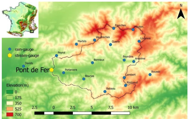
Le bassin versant de Real Collobrier est un site idéal pour tester les modèles pluie-débit. Ce bassin est étudié depuis plus de 50 ans par IRSTEA (Folton et al., 2018) et de nombreuses données sont directement disponibles par Internet. Dix-sept pluviomètres ont été installés sur le plus grand bassin versant (70 km2_{), et les débits ont été mesurés aux exutoires de onze}

sous-bassins, ce qui permet de comparer la calibration du modèle à l'échelle de quelques kilomètres carrés ou dizaines de kilomètres carrés dans une zone géographique réduite et d'évaluer la variabilité spatiale des paramètres. Dans cette étude, nous avons retenu 4 sous-bassins versants: Pont de Fer (70 km2_{), Rimbaud (1,5 km}2_{), Maurets (8,4 km}2_{) et Malière}

(12,4 km2_{) pour étudier également la variabilité spatiale des paramètres du modèle. Ces}

sous-bassins ont fait l’objet de nombreuses études et ont permis de mieux comprendre ce qui a permis de répondre à de nombreuses questions. (Taha et al., 1997 ; Gresillon et al., 1995)

Les performances du modèle peuvent être soigneusement estimées, tant en termes de capacité à reproduire les crues qu'en termes de variabilité spatiale des paramètres. En outre, les performances du modèle peuvent également être évaluées pour différentes densités de pluviomètres, ce qui donne une estimation des poids des incertitudes liées aux précipitations et des limites du modèle. L'objectif de cette thèse était d’appliquer un modèle pluie-débit distribué spécifique pour étudier les points suivants: (i) la capacité d'un modèle événementiel distribué, à simuler les crues éclair en climat méditerranéen, (ii) les règles de variabilité spatiale et temporelle des paramètres du modèle (iii) la capacité de modèle à être appliqué à des bassins non jaugés. L’étude a porté non seulement sur les bassins versants

(11)

ix

de Real Collobrier, mais également sur d’autres bassins versants de la Méditerranée (Figure 1), afin d’envisager une autre échelle de bassins dont la superficie couvre des centaines de kilomètres carrés et d’obtenir un échantillon cohérent de bassins pour la comparaison des performances et des paramètres du modèle. Sept bassins versants supplémentaires ont été étudiés (Gardon à Anduze, Ardèche à Vogüe, Allier à Langogne, Tarnon à Florac, Vidourle à Sommières, Verdouble à Tautavel, Aille à Vidauban). Des données sur ces bassins ont déjà été traitées dans la base de données de bassins versants de la plate-forme de modélisation ATHYS (www.athys-soft.org).

Différents modèles ont été testés en zone méditerranéenne : TOP MODEL (Piñol et al., 1997, Blöschl et al., 2008; Durand et al., 1992; Saulnier et Le Lay, 2009); MARINE (Estupina-Borrell et al., 2006; Roux et al., 2011). Le modèle événementiel distribué SCS-LR a été sélectionné dans notre étude, en raison de son caractère parcimonieux et de sa structure extrêmement simplifiée.

(12)

x

Principaux résultats

Calibration du modèle SCS-LR sur le bassin du Real Collobrier à Pont de

Fer

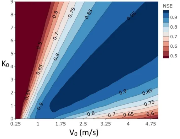
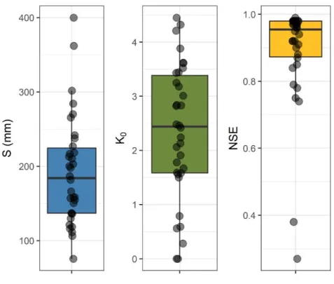
Une étude de sensibilité préalable montre que le modèle SCS-LR comporte 2 paramètres principaux : S, la capacité maximale de stockage en eau au débit de l’épisode, et K0 un

coefficient réglant la diffusion de la crue au cours du transfert (ou dans certains cas, V0 la

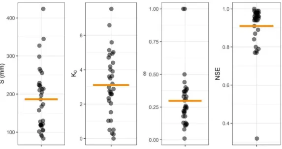
vitesse de transfert). À Pont de Fer, la calibration a été effectuée sur la base de 34 événements pluie-débit. Les paramètres du modèle ont été optimisés pour chaque événement. Avec les paramètres optimisés, l’erreur commise sur la simulation des débits variait de 0.27 à 0.99 au sens du critère de Nash-Sutcliffe (NS) pour l’ensemble des événements (médiane = 0.96, quartile inférieur = 0.87). Les plus faibles valeurs de NS correspondaient à des événements se produisant dans les conditions de sol initiales les plus sèches. Dans ces cas, les valeurs de faible débit ont été surestimées, alors que les valeurs de débit de pointe ont été sous-estimées.

Relation avec les conditions initiales

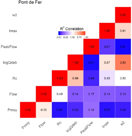
Après la calibration du modèle, il est apparu que S était le paramètre le plus variable et le plus influent pour les simulations. S correspond au déficit en eau au début de l’événement, de sorte qu’il devait être fortement dépendant des événements précédents et de l’état initial de saturation du sol. Nous avons donc essayé de trouver des relations entre S et deux indices supposés exprimer la teneur en eau initiale: le débit de base et la teneur en eau volumétrique

w2 au début de l’événement simulé. Pour le bassin du Real Collobrier à Pont de Fer, les deux

indices ont donné lieu à une corrélation relativement forte avec la rétention d’eau maximale, avec un coefficient de corrélation R2_{=0.85 entre S et log}₁₀_{Qb et 0.77 entre S et w}₂_.

Score prédictif du modèle

Ces relations peuvent être utilisées pour évaluer la précision réelle du modèle en mode projet. La précision réelle du modèle doit en effet être estimée par le NS calculé avec les valeurs prédites de S, au lieu des valeurs optimisées de S. On calcule dans ce cas de NS prédictif (pour tous les événements, la valeur médiane de K0 a été utilisée). Le NS prédictif

(13)

xi

la relation entre S et la teneur en eau w2 (au lieu 0.94 pour le NS médian calculé avec les

valeurs optimales de S et de la valeur médiane de K0).

Incertitude des précipitations

De plus, le grand nombre de postes pluviométriques installés sur le Real Collobrier nous a permis de tester l’effet de la densité de pluviomètres sur la calibration et la qualité du modèle. Les résultats ont montré que la réduction de la densité des pluviomètres influait à la fois sur la fonction d’erreur NS du modèle et sur l‘évaluation des paramètres du modèle. Lorsqu’on utilise un seul pluviomètre pour la calibration du modèle, les estimations de S peuvent varier de 250 à plus de 600 mm pour les sols initialement secs et de 50 à plus de 150 mm pour les sols initialement humides, en fonction du pluviomètre sélectionné. Les scores prédictifs NS du modèle évoluent entre 0.44 et 0.81 lorsqu’on ne considère qu’un seul des 17 pluviomètres sur le bassin.

Calibration du modèle sur les sous-bassins du Real Collobrier

Le modèle a ensuite été calibré sur trois sous-bassins supplémentaires du Real Collobrier : Rimbaud, Maurets, Malière. Les performances du modèle sont légèrement moindres que sur le bassin du Real à Pont de Fer, mais restent comparables. Les valeurs médianes de S diminuent avec les coefficients de ruissellement médians. On note toutefois que le bassin de Maurets présente un coefficient médian supérieur aux autres bassins et un S médian également supérieur. Les régressions entre S et les descripteurs w2 et débit de base sont très

voisines pour Pont de Fer et Rimbaud d’une part, et Maurets et Malière d’autre part. Les différences de Rimbaud avec Malière et Maurets pourraient être dues au fait que Rimbaud est représentatif de versants amont pentus productifs, alors que Malière et Maurets comprennent à la fois les mêmes versants pentus que Rimbaud à l’amont, et des unités peu productives à l’aval. La variabilité spatiale du paramètre K0 a été attribuée à un effet d’échelle

affectant la version initiale du modèle, qui a été corrigé.

Variation spatiale du paramètre S dans les bassins méditerranéens

La calibration du modèle a finalement été étendue à des bassins méditerranéens de plus grandes superficies. La valeur médiane de S variait d'un bassin à l'autre (Figure 2). La valeur la plus élevée de S appartenait à l’Allier, alors que le bassin versant d’Aille avait la valeur la plus faible. L'une des raisons de la valeur élevée du paramètre S dans le bassin de l'Allier

(14)

xii

pourrait être due au fait que les sols de ce bassin sont très perméables. Ils peuvent donc absorber une forte proportion de précipitations et alimenter des aquifères profonds. Le bassin versant de l'Aille est un bassin, dont la géologie est différente de celle des autres: on sait que ces grès du Permien génèrent des sols peu perméables de couleur rouge, comme dans la région de Lodève et Salagou, dans le département de l'Hérault (Brunet et Bouvier, 2017).

Figure 2 : Variabilité du paramètre S sur 11 bassins versants

La comparaison de la valeur S médiane et du coefficient de ruissellement médian pour chaque bassin montre cependant que ces variables sont peu corrélées. Cela pourrait s'expliquer par le fait que le coefficient de ruissellement intègre la réponse rapide et la réponse lente du bassin, tandis que S n'exprime que la réponse rapide du bassin. Par exemple, les bassins versants de l’Allier et de l’Aille ont un coefficient de ruissellement élevé similaire, mais pour des raisons différentes: les sols du bassin de l’Allier étaient supposés avoir une grande capacité de stockage de l’eau, mais aussi une grande capacité à produire de l’écoulement retardé par drainage des sols, alors que les sols peu perméables du bassin de l’Aille génèrent principalement du ruissellement superficiel ; ils ne peuvent stocker

(15)

xiii

beaucoup d'eau en raison de leur imperméabilité, et par conséquent ne libèrent que peu d’écoulement retardé. Ceci souligne le rôle de la contribution des écoulements souterrains dans la simulation des débits. Nous avons donc conclu que l’interprétation S devait tenir compte du type de ruissellement dans le bassin versant.

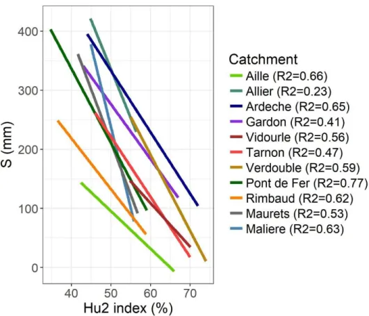
Afin de prendre en compte des facteurs secondaires spécifiques sur les bassins, notamment les conditions initiales de saturation des sols et leur impact sur la variabilité spatiale de S, nous avons ensuite considéré la variabilité spatiale des régressions entre S et les prédicteurs de la saturation des sols, débit de base et indice Hu2 (équivalent à w2).

Indice Hu2/w2

Les régressions entre les indices S et Hu2 de tous les événements sont significatives pour chaque bassin versant. Pour preuve, 9 des 11 bassins varient un coefficient de corrélation R2

supérieur à 0.5. La comparaison des droites de régression pour l’ensemble des bassins (Figure 3) montre des divergences de pentes et d’intercepts. Les régressions semblent être divisées en 2 groupes:

Allier, Maurets et Malière ont des pentes similaires, plus fortes que les autres. Les intercepts sont cependant différents.

Les autres bassins versants ont des pentes similaires, avec toutefois des intercepts différents, la valeur minimale étant obtenue pour le bassin de l’Aille, et la valeur maximale pour le bassin de l’Ardèche.

(16)

xiv

Figure 3 : Comparaison des régressions S-Hu2pour l’ensemble des bassins versants. Débit de base

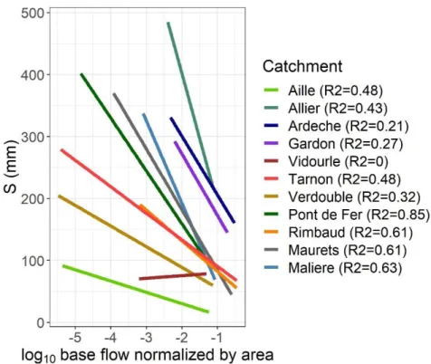
Le débit de base peut être considéré comme un autre indice pour expliquer la variabilité des événements du paramètre S. Les corrélations entre S et le débit de base sont généralement significatives, mais médiocres dans certains cas, notamment le bassin du Vidourle (R2=0). Les meilleurs scores ont été obtenus pour les bassins versants du Real Collobrier (0.61 à 0.86), alors que les autres bassins versants de la Méditerranée avaient un R2_{inférieur à 0.5. La comparaison des régressions sur l’ensemble des bassins (Figure 4)}

montre que les relations peuvent être très différentes d’un bassin à l’autre, et ne font pas apparaître un schéma régional (même si Allier, Gardon et Ardèche sont géographiquement proches et montrent des régressions similaires). Pour tenir compte des différentes superficies des bassins, le débit de base a été rapporté à la superficie du bassin, et désigne donc le débit spécifique de base.

(17)

xv

Figure 4 : Comparaison des régressions S-Qb pour l’ensemble des bassins versants

D'autres tentatives ont été faites pour utiliser un débit de base normalisé en divisant par le débit de base moyen, sans pour autant permettre de faire clarifier le schéma régional.

Discussion et conclusion

Le présent travail a permis une analyse détaillée des performances du modèle SCS-LR sur un ensemble de bassins méditerranéens, tant sur le plan de la capacité du modèle à simuler les crues que sur la variabilité spatiale des paramètres du modèle. Pour répondre aux questions énumérées dans les parties objectives du chapitre 1, nous présentons ici les principales conclusions et résultats, en premier lieu, pour le bassin versant de Real Collobrier:

1) Les résultats de notre étude ont prouvé que le modèle SCS-LR pouvait simuler une crue éclair en Méditerranée avec une grande précision. Le modèle ne nécessite qu’un petit nombre de paramètres et peut être calibré avec des données facilement accessibles. La calibration du modèle sur le Real Collobrier et d'autres bassins méditerranéens a donné des résultats positifs avec des valeurs élevées de NS ainsi que des valeurs élevées de R2_{pour la}

(18)

xvi

corrélation entre S et les prédicteurs de la saturation initiale du bassin dans la plupart des cas.

2) les données de précipitations denses sur le Real Collobrier, nous ont permis de tester l’effet de la densité des pluviomètres sur les résultats de la simulation. Les résultats ont montré que la réduction de la densité des pluviomètres influait à la fois sur la régression avec les conditions initiales et sur les paramètres calibrés du modèle. La diminution du nombre de pluviomètre a entraîné le changement des paramètres du modèle et la diminution du coefficient de corrélation R2_{. Ce résultat conduit à la conclusion que la comparaison des}

performances du modèle d’un bassin à l’autre peut être faussée lorsque les densités pluviométriques sont différentes

3) La variabilité spatiale du paramètre de transfert K0 dans le modèle initial était

initialement due à un effet d’échelle. La solution proposée a consisté à modifier la relation entre le temps de propagation Tm et le temps de diffusion Km du modèle Lag et Route. La

variabilité spatiale de K0 apparaît ainsi considérablement diminuée, et peut finalement être

reliée à la pente du bassin versant.

4) pour les bassins versants du Real Collobrier, la variabilité spatiale du paramètre de production S dans a été jugée cohérente avec la variabilité spatiale du coefficient de ruissellement. Cette relation n’a pas été vérifiée pour tous les bassins méditerranéens, et a conduit à penser que l’interprétation de S est dépendante du type de ruissellement généré dans le bassin.

5) La variation spatiale des régressions entre S et Hu2/w2 (ou débit de base) a conduit à

la conclusion qu'il était difficile de régionaliser ces régressions. Cet échec peut trouver son origine dans de multiples raisons :

- les incertitudes associées au prédicteur Hu2/w2, qui pourraient être dues au fait que les

mailles du modèle SIM sont trop grandes pour représenter les spécificités de petits bassins, ou au fait que les propriétés du sol utilisées dans SIM ne sont pas vraiment appropriées ou suffisamment précises pour représenter les propriétés réelles du sol.

- La mauvaise qualité de la mesure des débits de base, compte tenu de l’éventualité de mouvements des lits des rivières et de détarages fréquents de la courbe d’étalonnage des débits en basses-eaux, que des jaugeages trop peu nombreux ne permettent pas de suivre.

(19)

xvii

- De même, l’extrapolation de la courbe de tarage vers les débits de hautes-eaux est susceptible de générer sur certains bassins une forte incertitude, qui affecte directement l’estimation du paramètre S. Dans certains cas en effet (Gardon et Ardèche, par exemple), seulement quelques jaugages ont été utilisés pour établir la courbe de tarage.

- La raison peut aussi être liée aux incertitudes des précipitations. À l'exception du Real Collobrier, les autres bassins n'avaient pas une densité très élevée de pluviomètres. La variation de toutes les pentes et intercepts des régressions S-Hu2 ou S-Qb pour les bassins méditerranéens est assez similaire à celle des régressions établies en n’utilisant qu’un seul pluviomètre sur le Real Collobrier à Pont de Fer.

- La calibration des paramètres secondaires du modèle peut aussi être un problème. L’utilisation de Ia/S = 0.2, l’utilisation de paramètres constants, l’utilisation de S uniforme pour tout le bassin peuvent également conduire à une erreur lors de la calibration du paramètre S, puis affaiblir la corrélation entre S et les conditions initiales.

En conclusion et perspective, la calibration du modèle SCS-LR à l’aide d’observations pluies et débits permet de simuler les crues méditerranéennes avec une efficacité qui dépend de la densité des postes pluviométriques présents sur le bassin. La variabilité spatiale des paramètres du modèle reste difficile à interpréter, dans l’état des connaissances que nous avons des pluies, des débits et des caractéristiques hydrologiques des bassins versants. Les pistes d’amélioration consistent à tester de nouveaux indicateurs ou de mieux caractériser les propriétés des sols pour estimer la saturation initiale du bassin, à intégrer l’apport du radar météorologique pour la mesure des pluies, et à tester différentes spatialisations du paramètre S au sein des bassins.

(20)

xviii

List of abbreviations

Abbreviation Full name

ATHYS L'ATelier HYdrologique Spatialisé

CLC Corine land cover

CN Curve Number

DEM Digital Elevation Model

EM-DAT Emergency Events Database

IRD Institut de Recherche pour le Développement

IRSTEA Institut National de Recherche en Sciences et

Technologies pour l’Environnement et l’Agriculture

LR Lag & Route

NSE Nash–Sutcliffe Efficiency

RR Rainfall Runoff

SCHAPI Service Central d'Hydrométéorologie et d'Appui à la Prévision des Inondations

SCS Soil Conservation Services – Lag & Route

SIM SAFRAN-ISBA-MODCOU

(21)

xix

General introduction

Water is one of the essential elements of life, which without it humans cannot survive. However, the water-originated phenomena can also cause huge consequences, e.g. floods. Indeed, floods can severely damage both human lives and properties. This natural disaster is also inevitable, as currently there has not been any perfect way yet to prevent floods from occurring. Among different types of floods, flash flood is one of the most crucial types because of its characteristics of fast occurring.

According to the USA National Weather Service, “Flash flood is a flood caused by heavy or excessive rainfall in a short period of time, generally less than 6 hours. Flash floods are usually characterized by raging torrents after heavy rains that rip through river beds, urban streets, or mountain canyons sweeping everything in front of them. They can occur within minutes or a few hours of excessive rainfall. They can also occur even if no rain has fallen, for instance after a levee or dam has failed, or after a sudden release of water by a debris or ice jam” (https://www.weather.gov/mrx/flood_and_flash)

Flash flood causes many damages to the communities and the infrastructure (Gruntfest and Handmer, 2001). This type of natural phenomena has been shown to cause the highest mortality in a global assessment of flood-related casualties (Jonkman, 2005). In order to deal with floods in general and flash floods in particular, one of the most effective methods is to build the prediction systems. Many efforts have been invested in generating the database for flood researches and prediction. For instance, the Hydrometeorological Data Resources and Technologies for Effective Flash Flood Forecasting (HYDRATE) project was established in 2006 to understand better the hydro-meteorological processes leading to flash floods, which involves a multidisciplinary team of 17 organizations from 10 EU countries, China, USA, and South Africa. This project was also associated with the publicly accessible European Flash Flood Database, which aggregated all hydrometeorological data from the project (Borga et al., 2011). Moreover, the Hydrological Cycle in Mediterranean Experiment (HyMeX) program is a 10-year experimental effort (from 2010 to 2020) aiming to improve our understanding of the Mediterranean water cycle and its variability at different scales, which specially

(26)

3

focuses on hydro-meteorological extreme events and the associated social and economic vulnerability in the Mediterranean region (Drobinski et al., 2013). This program involves more than 400 scientists working in atmospheric sciences, hydrology, oceanography and social sciences from over 20 countries. An important part of the Hymex project - the Cévennes-Vivarais Mediterranean Hydro-meteorological Observatory aims to improve the knowledge and capabilities of hydrological risk prediction, which involves scientists from various disciplines, including meteorology, hydrology, geophysics, geography, applied mathematics and social sciences (Boudevillain et al., 2011). In addition, the EuroMedeFF dataset has collected flash flood hydrometeorological and geographical data, including high-resolution radar rainfall estimates and flood hydrographs from 49 high-intensity flash floods in the western and central Mediterranean, the Alps region and Continental Europe (Amponsah et al., 2018).

In spite of many efforts, current knowledge in flash flood prediction and risk assessment are still limited, which is mainly due to the lack of effective monitoring. Another inconvenience is the fact that the rain and stream gauges can be damaged when floods happen, which causes difficulties in maintaining the continuity of collected data, thus affecting the performance of flood simulating model. Moreover, the most vulnerable areas by flash floods are often where there is no data observed.

Thus, the concept of regionalization was proposed to help the prediction in the areas without available data (Blöschl and Sivapalan, 1995). This concept relies on the transfer of one or more particular parameters flood models from the catchment that have been already modeled to the new catchment (i.e. the one that lacks observed data). The regionalization process consists of two main steps. The first step is selecting a flood model which is sufficient for flash flood prediction. The possibility of improving this model should not be neglected. The second step is applying the selected model to at least one catchment to test their performance. The most important thing is the understanding of the variability of the parameters, thereby we can apply the regionalization. Several studies dealing with regionalization have been performed in France : Perrin, 2000 aimed to automatically calibrate several models over more than 1000 catchments, and relate the parameters to the catchments main characteristics (Perrin, 2000); Oudin et al., tested the performances of several regionalization methods such as geographical proximity, hydrological similarity and

(27)

4

multi-linear relationships with the catchment characteristics (Oudin et al., 2010); Vannier et al., dealt with the regionalization of the recession curves in Mediterranean catchments (Vannier et al., 2014); Garambois et al. compared the regionalization methods used by Oudin in a small set of Mediterranean catchments (Garambois et al., 2016). Besides, The SHYREG method (Aubert et al., 2014) which is a flood frequency analysis method was applied to 1605 basins in the French metropolitan territory for flood risk management. Our work intends to complete these previous works by analyzing the spatial variability of the runoff parameters in catchments of small and large areas (from a few to hundreds of squarekilometers).

Several models have been developed to study flash floods at various scales which was reported in (Javelle et al., 2018; Roux et al., 2011). However, there is still a debate on the question of which model is preferable, and which is not: continuous or event-based, empirical or physically-based, lumped or distributed models. As pointed out by (Oudin et al., 2010), a major concern about regionalization is due to equifinality of the parameters (Bardossy and Singh, 2008), that is a multiplicity of parameters satisfying to the goodness of the model. Equifinality can result from over parametrization of the model, thus it will be preferable to use parsimonious models when aiming to regionalization objectives. In addition, many uncertainties affect the input data used by the rainfall-runoff models, and can possibly originate artificial biases in the estimation of the model parameter, and their comparison from a catchment to another. So that each model would have to be tested and evaluated in highly documented sites where input and output data are observations are available and reliable, and where the uncertainties can be reduced as far as can be. It allows estimating in the one hand the actual performances of the model, and in the other hand simulating the impact of rainfall uncertainties for lower rain gauges density, which are representative of most of the catchments.

As a matter of fact, The Real Collobrier catchment is such a convenient site for modeling workbench. This catchment has been studied for more than 50 years by IRSTEA (Folton et al., 2018), and a lot of data are directly available from a website. Seventeen rain gauges have been settled over the larger catchment (70 km2_{). The discharges have been monitored in}

eleven sub-catchments, which allows comparing the model calibration at the scale of some square kilometers or dozen of square kilometers in a reduced geographical area and assess the spatial variability of the parameters. In such case, the performances of the model can be

(28)

5

carefully estimated, as well in terms of ability to reproduce the floods as in terms of applying the model in ungauged catchments. In addition, the performances of the model can also be compared for different dense rain gauges device, which gives an estimation of the weights of the rainfall uncertainties and the limitations of the model. The objective of this Ph.D. was to study a specific event-based distributed model in firstly the Real Collobrier to answer the following questions (i) how appropriate is an event-based distributed, but parsimonious model for flash flood prediction in Mediterranean climate, (ii) what is the impact of the uncertainty to the model calibration and (iii) how to explain the variability of these model’s parameters? The study dealt not only with the Real Collobrier catchments but also with other Mediterranean catchments, in order to consider another scale of catchments of which area covers hundreds of square kilometers and to obtain a consistent sample of catchments for the comparison of the model performances and parameters. 7 additional catchments have been considered (Gardon at Anduze, Ardèche at Vogüe, Allier at Langogne, Tarnon at Florac, Vidourle at Sommières, Verdouble at Tautavel, Aille at Vidauban. Data of these catchments have already been processed in the catchment database of the ATHYS platform www.athys-soft.org.

To fulfill the above objectives, the works are defined and described in this Ph.D. document is the composition of the following chapters:

Chapter 1 is a review of the literature and theoretical concepts on which the Ph.D. thesis is based. It introduces the water cycle’s processes, flood processes and the main factor that can affect flood. This chapter also mentions about Mediterranean flash floods and these consequences. Moreover, the hydrological model is described: the rainfall-runoff classification, modeling process and examples of rainfall-runoff model dealing with Mediterranean flash floods.

Chapter 2 provides the methodology of a parsimonious event-based rainfall-runoff model Soil Conservation Services – Lag & Route (SCS-LR) which are selected in the study. It also brings out the sensitivity test, the method of parameters assessment of the model.

Chapter 3 presents the Real Collobrier catchment and the results of the calibration of the model on the Pont de Fer sub-catchment. The chapter deals with various aspects: how the initial condition of the event-based model has to be set for each event, what is the actual performance of the model when using the predicted initial condition, what are the effects of

(29)

6

a reduction of the rain gauge density on the performances of the model as well as the parameters assessment.

Chapter 4 presents the spatial variability of the parameters at the sub-catchment scale. The results of the sub-catchments in Real Collobrier such as Pont de Fer, Rimbaud, Maurets, Malière are used. The range of area allows to test the hypothesis if the parameters are stable or not at this scale of the catchment, and if not, how can be explained the differences, for example in terms of numerical effects or hydrological effects.

Chapter 5 described the spatial variability of the parameters of the models at a higher scale, between Mediterranean catchments of which area extends from tenth to hundreds of square kilometers. The possibility of using predictors for applying the model in ungauged catchments is judged.

(30)

7

(31)

8

1 Introduction

This chapter presents the theoretical background and state of the art underpinning this work. The issue of the hydrological processes is reviewed in Section 1.1. In Section 1.2, the overview of the flood is indicated with the flood processes and the main factors affecting flood process. Then, the part of the model in general, hydrological model, model’s operation and the scaling issues and spatial-temporal variabilities is presented in Section 1.3. The following Section 1.4 reviews the knowledge about Mediterranean floods, as well as several previous studies about floods modeling in this region and the concept of regionalization.

1.1. Theoretical background: hydrological

processes in the drainage area

It has been well-known that the total mass of water on Earth does not significantly change over time (Skinner and Murck, 2011). However, the distribution of water into different forms and reservoirs is greatly variable, which mostly depends on the changes in climatic conditions. Indeed, water continuously moves and transforms between different reservoirs on Earth, including rivers, oceans, and atmospheres, via different physical processes, at the same time it transforms between different physical forms: liquid, solid and vapor. The continuous movement of water around the surface of the Earth is described by a concept called the water cycle. The water cycle involves the exchange of mass and energy and is also essential for the maintenance of all lives and ecosystems on this planet.

(32)

9

Figure 1.1: The water cycle on the catchment scale (From Winkler et al. 2010).

The different physical processes involved in the water cycle include precipitation, interception, evapotranspiration, condensation, infiltration, and percolation (Figure 1.1). Firstly, precipitation is the falling of any product of the condensed atmospheric water vapor under gravity (Deodhar, 2008), which occurs under the saturation of the atmosphere portion with water vapor. Precipitation can be divided into different categories based on the state of the water that falls off, including rain, drizzle, and snow (UNESCO and World Meteorological Organization, 1999). There are three mechanisms in which precipitation can occur, which differs in the direction of air movement, intensity, and duration, including convective, stratiform and orographic rainfall (Anagnostou, 2004; Dore et al., 2006).

However, only a part of precipitated water can reach the ground directly, while the rest is intercepted by vegetation and other surfaces. Interception is the interruption of movement of water from precipitation to stream channels, and it slows down the effect of precipitation. The precipitation that reaches the ground is called net precipitation. The part of the water that does not reach the ground directly can subsequently slide or drip from these surfaces to the ground, or it can be lost through evaporation. A part of water can fall to the forest floor

(33)

10

(through fall), run down branches and stems (stem flow), be absorbed by the vegetation, or remain on the surface of the foliage and branches and evaporate after the storm. The rain interception depends on storm intensity and duration, weather conditions (wind speed, air temperature, humidity), and amount and type of vegetation present (Crockford and Richardson, 2000).

The amount of precipitated water that reaches the ground directly or indirectly can be infiltrated into the soil. Infiltration is the movement of water through the boundary between the atmosphere and the soil, which is largely dependent on the soil surface conditions (Maidment, 1993). In particular, the porosity of the soil and the permeability of the soil affects the transfer of water. The infiltration rate also depends on the impact of the raindrops, the texture and structure of the soil, the initial soil moisture content. The maximum rate at which water can infiltrate into the soil is called the infiltration capacity (Winkler et al., 2010).

Infiltrated and stored water in the soil can later become subsurface runoff and contribute to streamflow. Streamflow is the flow or discharge of water along a defined natural channel. Streamflow is generated by a combination of runoff from the upstream watershed and return flow from the groundwater aquifer. Streamflow reflects the volume of the supplying water to a watershed (can be accounted by precipitation, evapotranspiration, infiltration) and also changes in the volume of other storages (lakes, aquifers, soil moisture). The streamflow rate at a particular point in time and space integrates all the hydrologic processes and storages upstream of that point. It depends on the sequence and size of rainfall events; seasonal distribution and nature of precipitation; the extent, type, and transpiration of covered vegetation; the soil infiltration capacity; and the topography of the watershed. (Maidment, 1993).

Infiltrated water can also percolate into deeper soil and rock layers through different layers of the soil due to gravity and capillary forces, then go to the groundwater. Groundwater is the water in the zone of saturation and completely fills the pores (Meinzer, 1923). Groundwater not only contributes to the stream base flow but also buffers peak flow when the bank sediments are sufficiently permeable (Winter et al., 2003). Depending on the relative water level, water can move from the groundwater to the stream or vice versa. The discharge of groundwater moving to the streams is commonly called base flow. This type of

(34)

11

flow occurs during the dry time of the year without specific storm events and seasonal phenomena.

The other part of precipitated water which is not infiltrated can directly contribute to stream flow or can also be stored in various type of water bodies such as lakes, swamps, ponds, and icebergs. A part of groundwater can also be considered as stored water.

The water which is infiltrated, stored, intercepted, and free in streamflow can return to the atmosphere by evapotranspiration in the form of water vapor. Evapotranspiration contains two main processes, evaporation and transpiration. Evaporation is the movement of water from intercepted rain and snow, as well as water bodies such as ponds, lakes, streams and even bare soil. Different important conditions are required for evaporation including (i) the availability of water, (ii) the humidity at the evaporative surface must be higher than that of the surrounding air, (iii) the energy to evaporate the water and (iv) the movement, or transfer, of water vapor away from the evaporative surface (Winkler et al., 2010). Therefore, the evaporation rate will increase when factors that induce those conditions occur, such as increasing solar radiation, air temperature, wind speed and decreasing atmospheric humidity (Condie and Webster, 1997). Transpiration accounts for the transfer of water from plant leaves through the stomata. The rate of this process depends strongly on the stomata, thus different plant species have different ability to regulate water loss. For example, trees usually have higher stomatal resistance to water loss than shrubs and grass (Kelliher et al., 1995). It is worth to note that transpiration rates decrease during rainfall due to the decreased vapor pressure gradient.

The amount of water that comes back to the atmosphere in the form of vapor can transform back to the liquid state by a process called condensation, forming dew, fog or clouds (McNaught and Wilkinson, 1997). Condensation occurs when the temperature of the air decreases or the amount of vapor increases up to its saturation points. This process releases an amount of heat which is previously required for evaporation. The most active particles forming clouds are sea salts, the atmospheric ions caused by lightning and the combustion products containing sulfurous and nitrous acids. These condensed water waits for the ideal condition to contribute to the water cycle as precipitation.

(35)

12

1.2. Overview of floods

1.2.1. Floods process

Extreme hydrological phenomena, including floods, are partly caused by the unequal geographical and geological distribution and movement of water. To decrease the damage of flood to humanity, the understanding of flood processes is very important. Initially, the definition of flood is expressed as the temporary rise in the level of a river. The flooding process can be explained below:

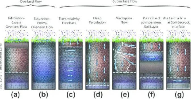
There are several mechanisms involved in the generation of runoffs (Figure 1.2). Each mechanism responds differently to rainfall in the flood variables: runoff volume, peak discharge and the timing of stream flow’s contributions in the channel. Climate, geology, topography, soil characteristic, vegetation, land use, and the intensity of events can also affect the relative dominance of each process.

(36)

13

1.2.1.1. Infiltration excess overland flow

Firstly, we have to mention the infiltration excess overland flow mechanism (Figure 1.3a). This mechanism is also called Hortonian overland flow because it was referred to by Robert E. Horton, one of the quantitative hydrology’s founding father in 1933. It was claimed that there is a maximum limiting rate for the soil in a given condition can absorb surface water input, so-called infiltration capacity. The excess water of the surface water input firstly accumulates on the soil surface and fills small depressions when it exceeds infiltration capacity. This part of water will evaporate or infiltrate later, thus it does not contribute directly to the overland runoff. However, if the surface water input continues to increase, the depression storage will also be filled, and the amount of water accumulated on the soil will start moving downslope, contributing to the overland runoff.

Infiltration excess runoff does not necessarily happen over a whole drainage basin area. Due to the spatial variability of the rainfall and soil properties, the area which contributed to infiltration excess runoff can only be a small part of the watershed (Betson, 1964). This concept is known as the partial-area infiltration excess overland flow.

The infiltration excess overland flow can occur anywhere that the water input excesses the infiltration capacity, most frequently in the area with having thin of devoid of plant cover. We can also see this process where the soil has been compacted or topsoil removed and in an urban area.

1.2.1.2. Saturation excess overland flow

In the place where infiltration capacity is very high, and the water input does not exceed infiltration capacity, overland flow can still occur by the water input on the area that is already saturated. Such mechanism is referred to as saturation excess overland flow (Figure 1.3b). This mechanism occurs when the infiltrated water has completely saturated the soil, or due to the rising of the water table, which make all surface water input become overland flow runoff.

Saturation excess overland flow is not restricted to near stream saturated zone although it is the most critical area. Saturation excess overland flow can also occur:

(37)

14

 where there are slope concavities which subsurface flow converge, thus water flows in faster than it can be transmitted downslope

 where the hydraulic gradient that induces subsurface flow in upslope is greater than that inducing downslope transmission

 where percolated water accumulates above the low-conductivity soil layers, forming perched zones of saturation due to decreasing hydraulic conductivity gradually with depth

1.2.1.3. Subsurface flow

The subsurface flow was mentioned above in the part of saturation excess overland flow. So, what is subsurface flow? Subsurface flow comes from the subsurface hydrologic processes, which are very complicated and unable to observe directly. The subsurface hydrologic processes are driven by many factors that influence the paths and rates of water movement. Therefore, subsurface flow is the major source of uncertainty in hydrologic models (Beven, 2012).

Subsurface flow occurs when water moves down a hillslope through soil layers or permeable bedrock to contribute to the runoff (Figure 1.3c-g). This process requires that the hydraulic lateral conductivity of the environment is larger than the vertical conductivity. Besides, subsurface flow is favored by the presence of impermeable shallow soil layers.

Subsurface flow can play the key role of flood runoff in humid environments and steep terrain with conductive soils (Anderson and Burt, 1990). We can see the subsurface flow in most upland terrain, and it may be dominant in humid regions with vegetal covering and well-drained soils. Meanwhile, this process can occur only under certain extreme conditions in lowland regions and in drier climates, for example, under high rainfall and high antecedent soil moisture.

(38)

15

Figure 1.3: (Rinderer et al., 2012) Different types of surface and subsurface runoff processes. (a) Overland flow is generated when the infiltration capacity of the soil layers at or near the surface is exceeded; (b) Overland flow can also be generated when the storage capacity of the soil layers at or near the surface is exceeded, (c) Lateral subsurface runoff increases when ground water rises into more transmissive soil layers, (d) Groundwater table tends to be low and soil water can percolate deep down into the soil or bedrock when the soil has coarse and highly permeable texture, (e) The flow rates toward the nearest stream channel can be high and subsurface runoff is generated when there are horizontal macropores, (f) A perched water table will form leading to lateral subsurface flow within the saturated soil layer when there exists water restricting layer in the soil profile, (g) lateral subsurface flow can also occur when there are water-restricting layers at the soil-bedrock interface.

The subsurface flows can accompany these mechanisms:

Piston effect: The piston effect assumes that water that falls on a slope is transmitted

downstream with a quasi-instantaneous pressure wave. It may cause a sudden exfiltration on the watershed.

Gravitational subsurface flow in macropores

Subsurface flow may be carried through macro pores which lead the water to unsaturated areas. Macropores are pores in which the capillarity phenomena do not exist. We can distinguish four types of macropores:

 Natural macropores: these macropores appear due to high initial hydraulic conductivity.

(39)

16

 Pores which formation is the result of micro soil fauna: these pores normally locate in the superior soil layer (0-100 cm) with a dimension of 1-50 mm.

 Pores which formation is due to vegetation roots. These pores normally become free when the plants die. Therefore, the structure of the macropores network of this type will depend on both the type of vegetation and its growing state.

 Cracks.

Figure 1.4: Pathways followed by a subsurface runoff on hillslopes (Kirkby, 1978)

Detailed cross-section through a hillslope that exposes in the pathways infiltrated water may follow as described in Figure 1.4. Infiltrated water may flow through the structural voids in the soil matrix, which are either small or large (macropores), including the opened passage in the soil caused by decaying roots and animals. Among these passages, subsurface

(40)

17

flow is favored by macropores. The different permeability of the horizontal soil matrix may lead to the build-up of a saturated wedge above a soil horizon interface. Water can either flow laterally from these saturated wedges through the soil matrix or enter the macropores in the soil, before going to the stream. Both processes mentioned above result in the subsurface flow called interflow.

Pipe flow

Another mechanism of subsurface flow is pipe flow. Pipe flow leads water to an unsaturated environment. This mechanism is similar to macro-pore to some extent, however, pipes are considered to be larger and more connective than macropores, as they can form a continuous network in the soil.

Transmissivity feedback

Subsurface flow can also occur by a mechanism called transmissivity feedback (Weiler and McDonnell, 2004). This phenomenon happens when water infiltrates rapidly along preferential pathways. This leads to the rapid rising of groundwater, reaching the highly permeable soil layers or macro-pore networks. As a consequent, water is then transmitted downslope (Figure 1.5).

Figure 1.5: (Tarboton, 2003) Schematic illustration of the macropore network being activated due to the rise in groundwater resulting in rapid lateral flow

Rapid lateral flow at the soil-bedrock interface

Another mechanism of subsurface flow, called lateral flow at the soil-bedrock interface (Weiler and McDonnell, 2004), occurs in regions with steep terrain, low permeability

(41)

18

bedrock and thin soil cover (Figure 1.6). In these regions, water can move rapidly through the thin soil layer and perch at the soil-bedrock interface. The addition of only a small amount of rainfall is enough to produce saturation at the soil-bedrock or soil-impeding layer interface because moisture content near the bedrock interface is often close to saturated.

Figure 1.6: Rapid lateral flow at the soil-bedrock interface (Tarboton, 2003) Subsurface stormflow by groundwater ridging

Figure 1.7: Groundwater ridging subsurface stormflow processes in an area of high infiltration (Tarboton, 2003). The shaded areas represent graphs of soil moisture at the base, middle and near the top of the hillslope (a) before the onset of rainfall; (b) as an initial response to rainfall; and (c) after continuing rainfall.

(42)

19

The processes involved in the generation of subsurface stormflow by groundwater ridging are illustrated in Figure 1.7. Before the onset of rainfall, the water table slopes slightly towards the channel to maintain the base flow of the stream (Figure 1.7a). When the rain starts, initially the water input leads the water table to rise near the stream but keep further upslope unchanged (Figure 1.7b). This leads to the increase of hydraulic gradient between groundwater and stream, resulting in the subsurface flow into the stream. As the rain continues, the water table rises to the surface over the lower part of the hillslope and the saturated area is expanding uphill. The water arises from this saturated area and runs downslope called return flow (Figure 1.7c). In this case, there is also direct precipitation onto the saturated zone which forms saturation excess runoff.

1.2.2. Main factors affecting flood process

It is widely recognized that the two most important climate variables influencing runoff generation during floods are rainfall and initial condition. Therefore, in the following section, rainfall and soil moisture will be discussed in detail.

1.2.2.1. Rainfall

1.2.2.1.1. Rainfall characteristic

The most important factor that drives flood is precipitation. Flood properties have been shown that be influenced by a combination of precipitation characteristics including the amount, intensity, duration, and spatial distribution. Moreover, the time of the rains and the area covered by the rain are also essential. The importance of each factor is not easy to separate and evaluate.

Rainfall intensities are one of the important factor leading to flooding generation in all catchment sizes (Costa, 1987; Pitlick, 1994; Schick, 1988). The higher rainfall intensity likely leads to higher potential runoff. Short and intense storms can generate the highest channel discharge, despite low total rainfall and storms with long durations or with greatest total rainfalls in the condition of uniform spatial distributions tended to produce moderate discharge events (Martı́n-Vide et al., 1999). However, it was reported that floods can be related to the total rainfall occurring than to intensity of an event (Bracken et al., 2008).