The magnetopause shape and location: a comparison of the Interball and Geotail observations with models

(1)

HAL Id: hal-00318821

https://hal.archives-ouvertes.fr/hal-00318821

Submitted on 1 Jan 2002

HAL is a multi-disciplinary open access

archive for the deposit and dissemination of

sci-entific research documents, whether they are

pub-lished or not. The documents may come from

teaching and research institutions in France or

abroad, or from public or private research centers.

L’archive ouverte pluridisciplinaire HAL, est

destinée au dépôt et à la diffusion de documents

scientifiques de niveau recherche, publiés ou non,

émanant des établissements d’enseignement et de

recherche français ou étrangers, des laboratoires

publics ou privés.

The magnetopause shape and location: a comparison of

the Interball and Geotail observations with models

J. Safránková, Z. N?me?ek, S. Du?ik, L. P?ech, D. G. Sibeck, N. N. Borodkova

To cite this version:

J. Safránková, Z. N?me?ek, S. Du?ik, L. P?ech, D. G. Sibeck, et al.. The magnetopause shape and

location: a comparison of the Interball and Geotail observations with models. Annales Geophysicae,

European Geosciences Union, 2002, 20 (3), pp.301-309. �hal-00318821�

(2)

Annales

Geophysicae

The magnetopause shape and location: a comparison of the

Interball and Geotail observations with models

J. ˇSafr´ankov´a1, Z. Nˇemeˇcek1, ˇS. Duˇs´ık1, L. Pˇrech1, D. G. Sibeck2, and N. N. Borodkova3

1_{Charles University, Faculty of Mathematics and Physics, V Holesovickach 2, 180 00 Praha 8, Czech Republic} 2_{Applied Physics Laboratory, JHU, Laurel, Maryland, USA}

3_{Space Research Institute, Moscow, Russia}

Received: 29 January 2001 – Revised: 15 October 2001 – Accepted: 23 October 2001

Abstract. A number of magnetopause models have been de-veloped in the course of last three decades. We have cho-sen seven of them and tested them using a fresh set of mag-netopause crossings observed by Interball-1, Magion-4, and Geotail satellites. The crossings cover the magnetopause from the subsolar region up to near-Earth tail (XGSE ∼ −20 RE) and all geomagnetic latitudes. Our study reveals

that (1) the difference between investigated models is smaller than the error of prediction caused by the factors not included in models, (2) the dayside magnetopause is indented in the cusp region, (3) the deepness of the indentation can reach ∼ 4 RE, and (4) the dimensions of the indentation do not

depend on the dipole tilt, whereas its location does.

Key words. Magnetopause, magnetospheric physics, solar wind

1 Introduction

In magnetospheric physics, it is important to have an accurate model for the determination of the size and shape of the netopause. In the absence of solar wind coupling to the mag-netosphere, these parameters could be predicted by the dy-namic and static pressures of the solar wind and the magnetic pressure of the magnetosphere. Based on this assumption, various models have been developed in the past. The earlier statistical study and following empirical model of the aver-age magnetopause shape and size was carried out by Fair-field (1971). Other empirical models followed; Formisano et al. (1979) adopted Fairfield’s approach and used nearly all magnetopause crossings available at that time to develop a new model. Detailed studies of magnetopause processes have shown that dayside reconnection leads to the changes of the magnetopause shape and location. For this reason, Sibeck et al. (1991) fitted magnetopause crossings as either a function of dynamic pressure or as a function of the BZ Correspondence to: J. ˇSafr´ankov´a

(jana.safrankova@mff.cuni.cz)

component of the interplanetary magnetic field (IMF) and Petrinec et al. (1991) fitted the magnetopause as a function of dynamic pressure for strongly northward and strongly south-ward IMFs separately.

Recent empirical magnetopause models are already bi-variate with respect to both dynamic pressure and IMF BZ

(e.g. Roelof and Sibeck, 1993; Petrinec and Russell, 1993, 1996; Kuznetsov and Suvorova, 1996; Shue et al., 1997; and Alexeev et al., 1999). The Howe and Binsack (1972) and Petrinec and Russell (1996) models of the nightside magne-topause use inverse trigonometric functions. The other men-tioned models adopted either the general equation of an ellip-soid with two parameters (eccentricity and standoff distance) or the general quadratic equation; Shue et al. (1997) used the standoff distance and the level of tail flaring.

From this short survey, it follows that these models use various functional forms to represent the shape and location of the magnetopause and are usually parametrized by solar wind dynamic pressure and IMF BZ. The basic findings of

these studies were that the magnetopause scales are roughly with pressure as p−1/6(p−1/6.6in Shue et al., 1997) and that for decreasing IMF BZ, the magnetopause displaces inward

near the nose and outward down the tail. However, the var-ious models have different ranges of validity (both spatially and in control parameters) because, among other things, the data sets used for their development were different. More-over, the data sets used for the development of models usu-ally contained a rather small number of high-latitude magne-topause crossings.

Sotirelis and Meng (1999) presented a calculation where the shape of the magnetopause is computed from the require-ment that the pressure in the magnetosheath is balanced by magnetic pressure inside the magnetosphere. The authors found changes in the shape of the magnetopause with vary-ing dipole tilt angle. The magnetotail and standoff location shifted vertically, in opposite directions, for nonzero dipole tilt. The vertical offset of the standoff location from the Earth-Sun line varies linearly with dipole tilt angle, reaching ∼3 RE for maximum of the tilt and having a weak

(3)

depen-302 J. ˇSafr´ankov´a et al.: Magnetopause shape and location dence on solar wind dynamic pressure. The magnetic field

model used to obtain the magnetospheric magnetic pressure is a modified version of the T96 model (Tsyganenko, 1996). Similar shifts were reported by Tsyganenko (1998), who used a new method to model the effects of the planetary dipole tilt and the IMF related twisting of the cross-tail cur-rent sheet. He concentrated on a deformation, yielding the observed gradual deflection of the magnetotail away from the equatorial plane of the tilted planar dipole and found that the deformation affects not only the shape of the tail cur-rent sheet but the entire magnetosphere, including the mag-netopause, which shifts along the Z axis in the same di-rection and with the same amplitude as the cross-tail cur-rent sheet. The author found the Earth’s dipole tilt effect upon the position of the magnetotail boundary in the distance range −40 < XGSM< −20 RE but suggests tilt related

ef-fects on the shape of the magnetopause for other intervals of XGSM. Using the data from Hawkeye 1 latitude, high-apogee spacecraft, similar results were reported by Eastman et al. (2000).

Boardsen et al. (2000) prepared a new empirical model for the shape of the near-Earth high-latitude magnetopause which is parametrized by solar wind dynamic pressure, IMF BZ, and dipole tilt angle and found that dipole tilt angle and

solar wind dynamic pressure are the most significant fac-tors influencing the shape of the high-latitude magnetopause, whereas IMF BZdependence is separable only after the

ef-fects of the pressure and dipole tilt angle are removed. How-ever, this model covers only a high-latitude part of the mag-netopause in a limited range of the XGSEcoordinate.

As one can see from our short and non-complete list, the variety of models leads often to confusion for potential users. For this reason, we used a completely new set of the magne-topause crossings and compared their coordinates with pre-dictions of several magnetopause models with motivation to analyze deviations between measurements and models in different ranges of XGSE. The set consists of low-latitude as well as high-latitude crossings and it allows us to deter-mine differences between the low- and high-latitude magne-topause.

2 Data set and methodology

The basic data set includes a collection of the magne-topause crossings observed by the Interball-Tail project. Both Magion-4 and Interball-1 satellites were launched into an elongated elliptical orbit with inclination of 63◦_{, apogee}

of ∼ 195 000 km (∼ 30 RE), and perigee of ∼ 800 km

(∼ 0, 12 RE). Due to orbital parameters and their temporal

evolution, the satellites have scanned a broad range of local times throughout the magnetospheric tail toward the subso-lar region. These magnetopause crossings represent ∼ 1800 crossings of the Interball-1 satellite at low- and high-latitudes from August 1995 to October 1997, and ∼ 120 crossings of Magion-4, mainly at low-latitudes. It would be pointed out that both Interball-1 and Magion-4 crossed the high-latitude

magnetopause often in a close vicinity of the cusp or in the cusp itself. The seasonal evolution of the cusp location and the evolution of the spacecraft orbits go in the same direc-tion which yields good coverage of the magnetopause near the cusp and a lack of mid- and low-latitude crossings in the subsolar region. To improve the coverage of measurements at these latitudes, we have complemented our observations with the Geotail magnetopause crossings during the same time period (approximately ∼ 1700 crossings). All crossings were spread from the subsolar region to XGSE ≈ −20 RE

and occurred under various upstream conditions: the solar wind velocity varied from 300 to 700 km/s, density from 1 to 35 cm−3, and Mach number from 4 to 50. The set includes multiple crossings.

Interball-1 and Magion-4 magnetopause crossings were identified manually on the basis of observations of ion and electron energy spectra (Yermolaev et al., 1997; Sauvaud et al., 1997; Nemecek et al., 1997) and the magnetic field (Nozdrachev et al., 1998). Geotail magnetopause crossings were computed automatically on the basis of the magnetic field changes (Ivchenko et al., 2000). The solar wind and IMF data were taken from WIND that was used as a monitor. The time of propagation of the solar wind features from the WIND position to the location of a magnetopause crossing was computed as a two-step approximation from WIND solar wind velocity measurements. In this approximation, we sup-pose the solar wind velocity equal to 400 km/s and determine the time lag from the difference of spacecraft locations along the XGSE axis. Then we take the actual velocity measured at the lagged time and compute the new lag. A deceleration of the solar wind in the magnetosheath is neglected because an error caused by this deceleration would be smaller than uncertainties caused by oblique fronts of solar wind distur-bances. Values of the solar wind dynamic pressure and IMF data used for the comparison with models were computed as five-minute averages centered around the time estimated as given above.

For our magnetopause crossings, we have computed the predicted magnetopause positions according to following models:

– Formisano et al. (1979) (hereafter referred as F79) – use the second-order three-dimensional surface for a fit of the data normalized to the averaged solar wind dy-namic pressure, pSW.

– Sibeck et al. (1991) (hereafter referred as S91) – use six subsets according to IMF BZand fitted an ellipsoid of

revolution to each subset. The ellipsoid parameters are a function of pSW.

– Roelof and Sibeck (1993) (hereafter referred as RS93) – use an ellipsoid of revolution in solar-wind aberrated coordinates and expressed the pSWand BZdependence

of each of the three ellipsoid parameters as a second-order (6-term) bi-variate expansion in pSWand BZ.

– Kuznetsov and Suvorova (1996) (hereafter referred as KS96) – use two paraboloids for the fit of the

(4)

magne-topause surface. These paraboloids intersect for the an-gle θ ∼ 30◦_{(θ is an angle between X}

GSE and radius vector of the observed crossing). Fits are computed for two IMF BZorientations.

– Petrinec and Russell (1996) (hereafter referred as PR96) – this model expanded their previous models (Petrinec et al., 1991; Petrinec and Russell, 1993). The dayside (XGSE>0) and nightside (XGSE <0) parts are fitted separately in different coordinate systems. They use different functional forms for the expression of co-efficients of the fit for different signs of IMF BZ.

– Shue et al. (1997) (hereafter referred as S97) – intro-duce a new functional form which is characterized by two parameters, roand α, representing the standoff

dis-tance and the level of tail flaring. Both parameters are a function of IMF BZand dynamic pressure, pSW.

– Alexeev et al. (1999) (hereafter referred as A99) - use a paraboloid of revolution for northward and southward IMF, separately.

We describe the accuracy of prediction by a ratio of the predicted (Rmod) and observed (Robs) distance of the

magne-topause from the Earth’s center computed for each crossing and each model. The set of Rmod/Robsratios for a particular

model is then fitted by the Gauss function and two param-eters of the fit (half-width and center) are presented in the following tables (for further explanation see, Fig. 1).

The second part of the study is devoted to an analysis of the importance of different parameters on the uncertainty of the prediction. For this study, we have computed the relative deviation, 1 as:

1 =Rmod−Robs Rmod

(1) and plotted this relative deviation as a function of these pa-rameters.

3 A comparison of magnetopause models

Most of the investigated models are best fits of a large num-ber of magnetopause crossings. The various authors limited the validity of their fits to a range of upstream parameters and/or XGSE coordinates according to the coverage of their data sets, the behaviour of their fits, etc. These validity limits are shown in Table 1. We have sorted our data set in accor-dance with these constraints in order to check each particular model within the range of its declared validity.

Table 2 shows a comparison of models applied to our data set. The assumption behind the computations presented in Table 2 was that models describe the magnetopause location in GSE coordinates. We should note that the GSM coordi-nates would be better for a description of the magnetopause position (and they really are, as we will show in Sect. 4) but the tested models are axisymmetric with respect to the XGSE axis and thus there is no difference between the GSE

Table 1. Ranges of the validity of models

Model Range of

IMF BZ pSW XGSE

[nT] [nPa] [R_E]

Sibeck et al., 1991 -6 6 0.54 9.9 -20 12

Petrinec and Russell, 1996

-15 10 0.109 6 -20 12

Shue et al., 1997 -18 15 0.5 8.5 -20 12

Kuznetsov and Su-vorova, 1996

-8 — 0.5 25 -10 12

Roelof and Sibeck, 1993

-5 5 0.5 8 -20 12

Formisano et al., 1979 — — — — -20 12

Alexeev et al., 1999 — — — — -20 12

Table 2. Comparison of models in GSE coordinates

Model Center Half-width Number

of points

Sibeck et al., 1991 1.006 0.076 2931

1.012 0.068 3147

Shue et al., 1997 1.007 0.087 3201

0.954 0.096 2223

1.007 0.075 3019

Formisano et al., 1979 0.978 0.073 3220

Alexeev et al., 1999 1.100 0.087 3175

and GSM coordinate systems. The only exception is the F79 model but this model is explicitly written in GSE.

As there are two parameters determining the accuracy of prediction, it is hard to say which model is better. We can note that the mean location of the magnetopause is described by a majority of the investigated models with ±3% error and the half-width of the distribution varies from 6.8 to 9.6%. The narrowest distribution is provided by the PR96 and F79 models. This fact is surprising because the F79 model is not parametrized by IMF BZ. The reason is that this model is

fully 3-D and accounts for the solar wind aberration caused by the Earth’s orbital motion, whereas all other models are axisymmetric, i.e. 2-D in nature. For this reason, we have rotated the coordinate system of the observed crossings in the ecliptic plane to remove this effect. Results of a com-parison of models with the observed crossings in aberrated coordinates are shown in Table 3. One can note an improve-ment of the prediction. This is valid for all models except F79 as one would expect.

The rotation of the coordinates in the ecliptic plane means that we are using coordinates aligned with averaged solar wind velocity because its vX coordinate dominates and the

average values of other two coordinates are near zero. How-ever, we are investigating the magnetopause locations in a

(5)

304 J. ˇSafr´ankov´a et al.: Magnetopause shape and location

Table 3. Comparison of models in aberrated coordinates

of points

Sibeck et al., 1991 0.995 0.078 2894

1.004 0.061 3002

Shue et al., 1997 0.999 0.073 3047

0.946 0.096 2256

0.995 0.072 2775

Formisano et al., 1979 0.971 0.088 3067

Alexeev et al., 1999 1.088 0.081 3044

particular place and time and the solar wind velocity affect-ing the magnetopause location has non-zero vY and vZ

com-ponents and they can change the actual magnetopause axis. We have rotated coordinates of the observed crossings into a new coordinate system in which the vY and vZ velocity

components vanished using 3-D WIND solar wind velocity measurements. A comparison of models with observations in this solar wind aligned coordinate system is shown in Table 4. One can see that the accuracy of prediction of almost all models is not better than that in Table 3.

We assume that the vY and vZ components of the solar

wind velocity are caused mainly by the presence of MHD waves in the flow. As these waves have a non-zero velocity of propagation in the plasma rest frame, we cannot predict the actual value of perpendicular velocity components simply by the time shift of data without an analysis of the propaga-tion of the waves. Moreover, the wave mode can change due to the interaction with the bow shock and thus the perpen-dicular velocity components in the magnetosheath can differ from those in the solar wind. It means that a rotation to the coordinates aligned with solar wind flow cannot bring a fur-ther improvement of the prediction, if a distant solar wind monitor is used. Thus, we neglect the perpendicular veloc-ity components and use the aberrated coordinated throughout the rest of the paper for all models except F79. The aberra-tion is an integral part of the F79 model and thus results of this model are presented in standard GSE coordinates.

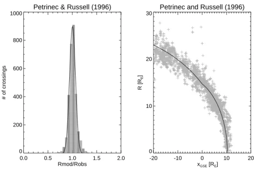
The distribution of the Rmod/Robs ratios for the PR96

model is plotted in the left part of Fig. 1. The parameters of the Gaussian fit plotted by a heavy line are listed in Table 3. The right part shows the position of the observed crossings around the model magnetopause surface. The position of the crossings was normalized with respect to the model. One can note a rather small spread of observations in the subsolar region which increases toward the tail.

In Table 5, we are analyzing several factors in order to find sources of this spread. The comparison of the dayside (XGSE >0) and nightside (XGSE<0) parts shows that both S97 and PR96 models reproduce the mean shape of the mag-netopause well but the uncertainty of S97 is higher in the

Table 4. Comparison of models in solar wind aligned coordinates

of points

Sibeck et al., 1991 1.000 0.077 2888

1.009 0.063 2990

Shue et al., 1997 1.002 0.074 3035

0.946 0.100 2274

0.999 0.074 2766

Formisano et al., 1979 0.974 0.089 3055

Alexeev et al., 1999 1.090 0.086 3030

nightside part. On the other hand, the nightside part is de-scribed better by S91 and RS93 models.

The magnetopause does not exhibit a significant dawn-dusk asymmetry in aberrated coordinates because the dis-tributions of the Rmod/Robs ratios peak at nearly the same

values for dawn and dusk crossings (RS93, PR96, S97). The aberration effect is well described by the model surface in F79 but this model places the magnetopause slightly farther from the Earth. The comparison of high and low-latitude crossings suggests an elliptic cross section of the magne-topause, being on average ∼ 5% flatter in the north-south di-rection. The same effect was analyzed in Sibeck et al. (1991) with a similar result but it has not been incorporated into their model. The F79 model includes but underestimates the men-tioned influence.

To analyze the influence of the upstream parameters, we have sorted out subsets of 500 crossings with lowest/highest solar wind dynamic pressure (lowest in the range of 0.4– 1.4 nPa and highest in the range of 3–6 nPa) and with high-est/lowest IMF BZ values. A comparison of the S97 model

with others (e.g. PR96 or S91) reveals that (pSW)1/6

proba-bly better describes the influence of the solar wind dynamic pressure than (pSW)1/6.6used in S97. All models except A99

slightly underestimate the influence of IMF BZon the

mag-netopause location; a best fit of this influence seems to be included in PR96.

In order to search for possible sources of uncertainties of predictions of different models, we have plotted results the same way as it is shown in Fig. 1 for the PR96 model. Af-ter an analysis of such plots (not presented), we can note that slightly better results provided by the PR96 model are caused by the fact that this model uses two different surfaces for the dayside and nightside magnetopause. The magnetopause shape is probably too complicated to be described by a sim-ple second order surface. The KS96 model uses two different surfaces too, but this model was developed for extreme high solar wind pressure and we have only a few such crossings in our data set.

As we noted above, the PR96 model provides the best description of the magnetopause surface. However, Fig. 1

(6)

Petrinec & Russell (1996) 0.0 0.5 1.0 1.5 2.0 Rmod/Robs 0 200 400 600 800 1000 # of crossings

Petrinec and Russell (1996)

-20 -10 0 10 20 xGSE [RE] 0 10 20 30 R [R E ]

Fig. 1. Histogram of Rmod/Robsratios for the PR96 model (left part) and the position of the observed magnetopause crossings in aberrated

coordinates scaled to the solar wind dynamic pressure and IMF BZ(right part). The heavy line represents the PR96 magnetopause under

standard conditions (pSW=2 nPa, IMF BZ=0).

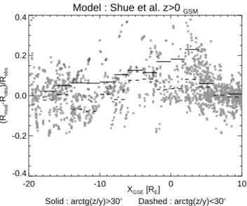
Model : Petrinec and Russell (1996) z>0 GSM

Solid : arctg(z/y)>30o Dashed : arctg(z/y)<30o -20 -10 0 10 XGSE [RE] -0.4 -0.2 0.0 0.2 0.4 (R mod -R obs )/R obs

Fig. 2. Distribution of relative deviations of the observed

magne-topause crossings from the PR96 prediction along aberrated XGSE

axis. Circles and the heavy line refer to high geomagnetic latitudes.

shows that the spread of observed crossings is rather high and many crossings are observed 2 or 3 REinside or outside

the model magnetopause surface.

4 The high-latitude magnetopause

As a next step, we have sorted the relative deviation, 1 ac-cording to different parameters and plotted it as a function of XGSE-coordinates. We have concentrated on the Northern Hemisphere (ZGSM ≥ 0) because our data set covers better

this hemisphere and the situation in both hemispheres can be different. Since our results in Table 5 suggest a change in the magnetopause shape with latitude, we have divided our data set into two groups: low-latitude part (arctan ZGSM/YGSM< 30◦) and high-latitude part (arctan ZGSM/YGSM>30◦).

Figure 2 depicts a comparison of the high- and low-latitude groups. We can point out that in the range of (XGSE ≤ 3), the mean values of 1 for low-latitude crossings (dashed line) lie near zero and below that for high-latitudes. Taking into account a definition of 1, we can conclude that the PR96 model well describes the shape of the nightside low-latitude magnetopause, whereas the high-latitude magnetopause lies on average inside the predicted position. The difference is ∼ 3 − 15% with a trend to decrease down the tail. At the subsolar region (XGSE ≥ 5), the difference between low-and high-latitudes seems to be negligible.

The most pronounced difference between high- and low-latitudes is observed in the region (−5 ≤ XGSE ≤ 5). The low-latitude crossings decline from prediction by ∼ 7% on average (dashed line) but the high-latitude crossings are sys-tematically observed nearer to the Earth than predicted. The peak of 1 is ∼ 22% at XGSE = +3.

The greatest deviation of the prediction from observations is seen near XGSE ∼ 0 where the functional form of PR96 changes and we suppose that this fact could influence the re-sults. For this reason, Fig. 3 shows the same plot as Fig. 2 for S97 which uses the same function throughout the whole range of XGSE. However, we can note similar behaviour for 1 at high-latitudes. We tested all models and the re-sults were qualitatively similar, and thus we have chosen the PR96 model for further demonstration. The location of the region with greatest deviation of observations from the model

(7)

306 J. ˇSafr´ankov´a et al.: Magnetopause shape and location

Model : Shue et al. z>0 GSM

Solid : arctg(z/y)>30o_{Dashed : arctg(z/y)<30}o

-20 -10 0 10 XGSE [RE] -0.4 -0.2 0.0 0.2 0.4 (R mod -R obs )/R obs

Fig. 3. The same as Fig. 2 for the S97 model.

Model : Petrinec and Russell arctg(z/y)>30o

GSM

Solid : tilt>0 Dashed : tilt<0

-20 -10 0 10 XGSE [RE] -0.4 -0.2 0.0 0.2 0.4 (R mod -R obs )/R obs

Fig. 4. Comparison of the magnetopause locations for positive

(solid line, circles) and negative (dashed line, asterisks) tilt angles at high latitudes.

in high-latitudes and in a limited range of XGSEsuggests that the magnetopause is indented due to the presence of the cusp. This suggestion confirms Fig. 4 where the high-latitude data are plotted for positive and negative tilts. The averaged val-ues show that the indented region shifts sunward for positive tilt as one would expect, if the cusp is a source.

Earlier studies of the cusp precipitation reveal an equator-ward shift of the cusp region when IMF BZbecomes

nega-tive. Figure 5 shows a comparison of the magnetopause lo-cations for different IMF BZorientation. It is hard to say if

the dependence in Fig. 5 confirms this effect for the magne-topause because our data set suffers from poor data coverage in the range 0 < XGSE < 2. We can note that during in-tervals of negative IMF BZthe indentation either shifts more

sunward or becomes broader.

Model : Petrinec and Russell z>0 arctg(z/y)>30o

GSM Solid : Bz>0 Dashed : Bz<0 -20 -10 0 10 XGSE [RE] -0.4 -0.2 0.0 0.2 0.4 (R mod -R obs )/R obs

Fig. 5. The same data as in Fig. 4 but sorted according to IMF BZ.

Model : Petrinec and Russell (1996) z>0 arctg(z/y)>30o

GSM Solid : dp>2 Dashed : dp<2 -20 -10 0 10 XGSE [RE] -0.4 -0.2 0.0 0.2 0.4 (R mod -R obs )/R obs

Fig. 6. The same data as in Fig. 4 but sorted according to solar wind

dynamic pressure.

Figure 6 shows the high-latitude crossings sorted accord-ing to solar wind dynamic pressure. The averaged 1 does not exhibit any systematic dependence on the nightside magne-topause (XGSE<0). However, on the dayside (0 ≤ XGSE≤ 6), the solar wind pressure effect seems to be stronger than the model predicts because the crossings observed under higher pressure (heavy line) exhibit higher 1. However, the number of points is rather low and the difference lies in the range of most probable error.

We have analyzed the low-latitude crossings the same way but we did not find any notable change of the profile of 1 with solar wind dynamic pressure, tilt angle, or IMF BZ.

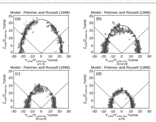
A view on the extent of the cusp indentation is shown in Fig. 7. The coordinates of crossings were normalized to the

(8)

Table 5. Comparison of models under different constraints (X, Y , Z – aberrated coordinates; C – center of distribution; HW – half-width of

distribution of Rmod/Robsratios)

Model Conditions

X >0 X <0 Y >0 Y <0 low lat high lat BZ(min) BZ(max) pSW (min) pSW (max)

C HW C HW C HW C HW C HW C HW C HW C HW C HW C HW S91 1.005 0.092 0.988 0.064 1.007 0.081 0.987 0.075 0.980 0.079 1.021 0.060 1.001 0.089 0.971 0.069 0.994 0.077 0.996 0.079 PR96 0.999 0.063 1.009 0.059 1.006 0.062 1.003 0.061 0.991 0.061 1.028 0.053 1.008 0.071 1.000 0.062 1.017 0.070 1.002 0.063 S97 0.998 0.058 1.000 0.092 1.003 0.072 0.996 0.073 0.986 0.064 1.034 0.078 1.007 0.089 0.989 0.084 0.991 0.078 1.020 0.080 KS96 0.951 0.104 0.938 0.080 0.960 0.102 0.937 0.091 0.933 0.090 0.993 0.101 0.903 0.098 0.980 0.078 0.936 0.089 0.950 0.103 RS93 0.985 0.078 1.005 0.067 1.004 0.076 0.990 0.069 0.978 0.067 1.030 0.060 1.006 0.068 0.986 0.069 0.963 0.069 1.018 0.071 F79 0.979 0.058 0.982 0.088 0.982 0.073 0.981 0.074 — — — — 0.981 0.071 0.981 0.076 — — — — A99 1.068 0.083 1.107 0.073 1.096 0.087 1.083 0.078 1.069 0.074 1.131 0.068 1.013 0.088 1.133 0.61 1.083 0.088 1.096 0.102

Model : Petrinec and Russell (1996)

x<-5 -30 -20 -10 0 10 20 30 YGSM/YGSM-Petr.*const 0 5 10 15 20 25 ZGSM /ZGSM-Petr. *const

-5<x<0 -30 -20 -10 0 10 20 30 YGSM/YGSM-Petr.*const 0 5 10 15 20 25 ZGSM /ZGSM-Petr. *const

0<x<5 -30 -20 -10 0 10 20 30 YGSM/YGSM-Petr.*const 0 5 10 15 20 25 ZGSM /ZGSM-Petr. *const

x>5 -30 -20 -10 0 10 20 30 YGSM/YGSM-Petr.*const 0 5 10 15 20 25 ZGSM /ZGSM-Petr. *const (d) (c) (b) (a)

Fig. 7. Projection of the observed magnetopause crossings along the model magnetopause surface (the PR96 model). The oblique straight

lines indicate 30◦of geomagnetic latitude. This angle is used as a breakpoint between low- and high-latitudes.

PR96 model: Yn= Yobs Ymod .Ymod(Xn) (2) Zn= Zobs Zmod .Zmod(Xn), (3)

where Y, Z are expressed in GSM coordinates and Xn

ac-quires values −10, −5, 0, and +5 RE for different panels.

This normalization projects all points of the model surface onto the heavy line depicted in the panels. The oblique straight lines indicate 30◦of geomagnetic latitude. This an-gle was used as a breakpoint between low- and high-latitudes in Figs. 2–6. The experimental points are spread around this line symmetrically in low-latitudes in all panels of Fig. 7. A similar conclusion is valid for high-latitude parts of the (a)

and (d) panels, whereas nearly all high-latitude crossings lie below the line in the (b) and (c) panels. This comparison of panels shows that the indentation of the magnetopause can be expected in the range from XGSE = −5 to XGSE = +5 RE

at magnetic latitudes higher than 30◦(straight thin lines) and its deepness can reach ∼ 4 RE.

5 Summary and conclusion

We have prepared a fresh set of the low- and high-latitude magnetopause crossings from Interball and Geotail observa-tions and complemented these data with 5-minute averages of the WIND solar wind and IMF measurements. An advan-tage of this set is that the magnetopause crossings as well

(9)

308 J. ˇSafr´ankov´a et al.: Magnetopause shape and location as the upstream conditions were determined using the same

methodology and the same upstream parameter monitor. This set has been used for the comparison of various mag-netopause models. However, our set contains only a few crossings observed under extreme conditions. For this rea-son, we have not tested the models dedicated predominantly to these conditions, e.g. Shue et al. (1998); Kuznetsov and Suvorova (1998); or Kawano et al. (1999). Moreover, ac-cording to Shue et al. (1998, 2000); Kuznetsov and Suvorova (1998), and Petrinec and Russell (1996), the models have al-most the same performance during normal solar wind condi-tions.

We can summarize our investigation as follows:

1. The “aberration” of the solar wind caused by the Earth’s orbital motion has a significant effect on the magne-topause location. On the other hand, the influence of the perpendicular components of the solar wind velocity re-mains under question. A more sophisticated method of the propagation of observations of a distant solar wind monitor toward the Earth is required in order to con-firm or exclude this effect. This partial conclusion is in agreement with the note in Boardsen et al. (2000). 2. From a general point of view, the PR96, RS93, S91,

and S97 models are close to each other in our ranges of coordinates (−20 RE ≤ XGSE ≤ 12RE) and

up-stream conditions (0.5 nPa≤ pSW < 6 nPa, −7 nT≤

BZ ≤ +9 nT). Taking into account both parameters

of the Gaussian fits (center and half-width), the PR96 model provides the best prediction but the differences between the aforementioned models are small. In gen-eral, the difference among their predictions is signifi-cantly smaller than the spread of observations caused by factors which are not included in the models. How-ever, this conclusion cannot be applied to any particular crossing.

3. The (pSW)1/6term probably describes the influence of

the solar wind dynamic pressure on the magnetopause location better than (pSW)1/6.6used in S97.

4. All investigated models except A99 slightly underesti-mate the IMF BZeffect. This is true for positive as well

as for negative BZ. However, the accuracy of the

predic-tions of the majority of models is better for southward IMF.

5. If the effect of the aberration is removed, the magne-topause does not exhibit any notable dawn-dusk asym-metry. The difference between both flanks is about 1%, comparable to its uncertainty, and thus it is in a range of the most probable error.

6. The high-latitude magnetopause cross section is flat-tened. The location of this depression is controlled by the tilt angle of the Earth’s dipole. A most probable source of the depression is the magnetospheric cusp. Our data show a similar depression for both signs of

the tilt, whereas Eastman et al. (2000) noted that when the dipole tilts away from the Sun, the indentation is re-duced. The problem of the cusp indentation has a long history and its presence was periodically suggested and then rejected. We assume that the indentation is narrow and its location varies with dipole tilt and upstream con-ditions and thus this region can be crossed by a space-craft only occasionally. Interball-1 was launched into the cusp region and thus its coverage of the cusp inden-tation for negative tilts is probably better than that of Hawkeye.

7. The indentation can be observed at geomagnetic lati-tudes higher than 30◦ and in a broad range of XGSE coordinates (−2 RE ≤ XGSE ≤ 8 RE). An averaged

deepness is ∼ 2.5 RE but the magnetopause was often

observed ∼ 4 REbelow the expected location

(accord-ing to PR96).

8. The position and deepness of the depression is in qual-itative agreement with the Sotirelis and Meng (1999) model and with the study of the magnetopause cross section in Sibeck et al. (1991).

9. The location and/or extent of the indentation seems to be controlled by the IMF BZcomponent.

10. The indented part of the magnetopause seems to be more sensitive to the changes in the solar wind dynamic pressure than other parts.

In order to be “user friendly”, the investigated models de-scribe the magnetopause with a simple second-order surface. Such a surface cannot reflect the observed indentation. It results in the fact that models put the low-latitude magne-topause at 1 − 3% nearer to the Earth than it is observed. The differences between models can be caused by a number of magnetopause crossings through the indented region used for the development of a particular model.

Acknowledgement. This work was supported by the Czech Grant Agency under Contracts 205/99/1712 and 205/00/1686 and by the Grant Agency of Charles University under Contract 181. Their fi-nancial support is greatly acknowledged. Authors are grateful to A. Lazarus and R. Lepping for the WIND plasma and magnetic field data and to L. Frank for the Geotail plasma data.

The authors thank both referees for their assistance in evaluating this paper.

Topical Editor G. Chanteur thanks two references for their help in evaluating this paper.

References

Alexeev, I. K., Kalgaev, V. V., and Lyutov, Yu. G.: The parabolic magnetopause form and location versus solar wind pressure and IMF, 9th Scientific Assembly of IAGA, Birmingham, A343, 19– 24 July, 1999.

Boardsen, S. A., Eastman, T. E., Sotirelis, T., and Green, J. L.: An empirical model of the high-latitude magnetopause, J. Geophys. Res., 105, 23 193, 2000.

(10)

Eastman, T. E., Boardsen, S. A., Chen, S.-H., Fung, S. F., and Kessel, R. L.: Configuration of high-latitude and high-altitude boundary layers, J. Geophys. Res., 105, 23 221, 2000.

Fairfield, D. H.: Average and unusual locations of the Earth’s mag-netopause and bow shock, J. Geophys. Res., 76, 6700, 1971.

Formisano, V., Domingo, V., and Wenzel, K.-P.: The

three-dimensional shape of the magnetopause, Planet. Space Sci., 27, 1137, 1979.

Howe, H. C. and Binsack, J. H.: Explorer 33 and 35 plasma ob-servations of magnetosheath flow, J. Geophys. Res., 77, 3334, 1972.

Ivchenko, N. V., Sibeck, D. G., Takahashi, K., and Kokubun S.: A statistical study of the magnetosphere boundary crossings by the Geotail satellite, Geophys. Res. Lett., 27, 2881–2884, 2000. Kawano, H., Petrinec, S. M., Russell, C. T., and Higuchi, T.:

Mag-netopause shape determinations from measured position and es-timated flaring angle, J. Geophys. Res., 104, 247, 1999. Kuznetsov, S. N. and Suvorova, A. V.: Empirical model of the

dayside magnetopause, INP MSU Preprint, 96–37/444, Moskva, 1996.

Kuznetsov, S. N. and Suvorova, A. V.: An empirical model of the

magnetopause for broad ranges of solar wind pressure and Bz

IMF, in: Polar Cap Boundary Phenomena, (Eds) Moen, J., et al., p. 51, Kluwer Acad., Norwell, Mass., USA, 1998.

Nemecek, Z., Fedorov, A., Safrankova, J., and Zastenker, G.: Struc-ture of the low-latitude magnetopause: Magion-4 observations, Ann. Geophysicae, 15, 553, 1997.

Nozdrachev, M. N., Skalsky, A. A., Styazhkin, V. A., and Petrov, V. G.: Some results of magnetic field measurements by the FM-3I flux-gate instrument onboard the Interball-1 spacecraft, Cosmic Research, 36, 268–272, 1998.

Petrinec, S. M., Song, P., and Russell, C. T.: Solar cycle variations in the size and shape of the magnetopause, J. Geophys. Res., 96, 7893, 1991.

Petrinec, S. M. and Russell, C. T.: Factors which control the size of the magnetosphere, in: Solar Terrestrial Predictions IV, vol. 2, (Eds) Hruska, J., et al., pp. 627–635, Natl. Oceanic and Atmos. Admin. Environ. Res. Lab., Boulder, Colo., 1993.

Petrinec, S. M. and Russell, C. T.: Near-Earth magnetopause shape

and size as determined from the magnetopause flaring angle, J. Geophys. Res., 101, 137, 1996.

Roelof, E. C. and Sibeck, D. G.: Magnetopause shape as a

bivari-ate function of interplanetary magnetic field Bzand solar wind

dynamic pressure, J. Geophys. Res., 98, 21 421, 1993.

Sauvaud, J.-A., Koperski, P., Beutier, T., Barthe, H., Aoustin, C., Thocaven, J. J., Rouzaud, J., Penou, E., Vaisberg, O., and Borod-kova, N.: The Interball-Tail ELECTRON experiment: initial re-sults on the low-latitude boundary layer of the dawn magneto-sphere, Ann. Geophysicae, 15, 587, 1997.

Shue, J.-H., Chao, J. K., Fu, H. C., Khurana, K. K., Russell, C. T., Singer, H. J., and Song, P.: A new functional form to study the solar wind control of the magnetopause size and shape, J. Geo-phys. Res., 102, 9497, 1997.

Shue, J.-H., Chao, J. K., Fu, H. C., Khurana, K. K., Russell, C. T., Singer, H. J., and Song, P.: Magnetopause location under ex-treme solar wind conditions, J. Geophys. Res., 103, 17 691, 1998. Shue, J.-H., Song, P., Russell, C. T., Chao, J. K., and Yang, Y.-H.: Toward predicting the position of the magnetopause within geosynchronous orbit, J. Geophys. Res., 105, 2641, 2000. Sibeck, D. G., Lopez, R. E., and Roelof, E. C.: Solar wind control

of the magnetopause shape, location, and motion, J. Geophys. Res., 96, 5489, 1991.

Sotirelis, T. and Meng, C.-I.: Magnetopause from pressure balance, J. Geophys. Res., 104, 6889, 1999.

Tsyganenko, N. A.: Effects of the solar wind conditions on the global magnetospheric configuration as deduced from data-based field models, in: Proceeding of Third International Conference on Substorms (ICS-3), Eur. Space Agendcy Spec. Publ., ESA SP-389, 181, 1996.

Tsyganenko, N. A.: Modeling of twisted/warped magnetospheric configurations using the general deformation method, J. Geo-phys. Res., 103, 23 551, 1998.

Yermolaev, Yu. I., Fedorov, A. O., Vaisberg, O. L., Balebanov, V. M., Obod, Yu. A., Jimenez, R., Fleites, J., Llera, L., and Omelchenko, A. N.: Ion distribution dynamics near the Earth’s bow shock: first measurements with the 2D ion energy spectrom-eter CORALL on the Interball/Tail-probe satellite, Ann. Geo-physicae, 15, 533, 1997.