HAL Id: hal-01083697
https://hal-polytechnique.archives-ouvertes.fr/hal-01083697
Submitted on 26 Apr 2021
HAL is a multi-disciplinary open access
archive for the deposit and dissemination of
sci-entific research documents, whether they are
pub-lished or not. The documents may come from
teaching and research institutions in France or
abroad, or from public or private research centers.
L’archive ouverte pluridisciplinaire HAL, est
destinée au dépôt et à la diffusion de documents
scientifiques de niveau recherche, publiés ou non,
émanant des établissements d’enseignement et de
recherche français ou étrangers, des laboratoires
publics ou privés.
reduction in solar irradiance and increase in CO2
Nicolas Huneeus, Olivier Boucher, Kari Alterskjaer, Jason N. S. Cole, Charles
L. Curry, Duoying Ji, Andy Jones, Ben Kravitz, Jón Egill Kristjánsson, John
C. Moore, et al.
To cite this version:
Nicolas Huneeus, Olivier Boucher, Kari Alterskjaer, Jason N. S. Cole, Charles L. Curry, et al.. Forcings
and feedbacks in the GeoMIP ensemble for a reduction in solar irradiance and increase in CO2. Journal
of Geophysical Research: Atmospheres, American Geophysical Union, 2014, 119 (9), pp.5226-5239.
�10.1002/2013JD021110�. �hal-01083697�
Forcings and feedbacks in the GeoMIP
ensemble for a reduction in solar
irradiance and increase in CO
2Nicolas Huneeus1,2, Olivier Boucher1, Kari Alterskjær3, Jason N. S. Cole4, Charles L. Curry5, Duoying Ji6, Andy Jones7, Ben Kravitz8, Jón Egill Kristjánsson3, John C. Moore6, Helene Muri3, Ulrike Niemeier9, Phil Rasch8, Alan Robock10, Balwinder Singh8, Hauke Schmidt9, Michael Schulz11, Simone Tilmes12, Shingo Watanabe13, and Jin-Ho Yoon8
1
Laboratoire de Météorologie Dynamique, IPSL/CNRS, UPMC, Paris, France,2Now at Department of Geophysics and Center for Climate and Resilience Research, University of Chile, Santiago, Chile,3Department of Geosciences, University of Oslo,
Oslo, Norway,4Canadian Centre for Climate Modelling and Analysis, Environment Canada, Toronto, Ontario, Canada,
5School of Earth and Ocean Sciences, University of Victoria, Victoria, British Columbia, Canada,6State Key Laboratory of
Earth Surface Processes and Resource Ecology, College of Global Change and Earth System Science, Beijing Normal University, Beijing, China,7Met Office Hadley Centre, Exeter, UK,8Atmospheric Sciences and Global Change Division, Pacific
Northwest National Laboratory, Richland, Washington, USA,9Max Planck Institute for Meteorology, Hamburg, Germany,
10Department of Environmental Sciences, Rutgers University, New Brunswick, New Jersey, USA,11Norwegian
Meteorological Institute, Oslo, Norway,12National Center for Atmospheric Research, Boulder, Colorado, USA,13Japan Agency for Marine-Earth Science and Technology, Yokohama, Japan
Abstract
The effective radiative forcings (including rapid adjustments) and feedbacks associated with an instantaneous quadrupling of the preindustrial CO2concentration and a counterbalancing reduction of thesolar constant are investigated in the context of the Geoengineering Model Intercomparison Project (GeoMIP). The forcing and feedback parameters of the net energyflux, as well as its different components at the top-of-atmosphere (TOA) and surface, were examined in 10 Earth System Models to better understand the impact of solar radiation management on the energy budget. In spite of their very different nature, the feedback parameter and its components at the TOA and surface are almost identical for the two forcing mechanisms, not only in the global mean but also in their geographical distributions. This conclusion holds for each of the individual models despite intermodel differences in how feedbacks affect the energy budget. This indicates that the climate sensitivity parameter is independent of the forcing (when measured as an effective radiative forcing). We also show the existence of a large contribution of the cloudy-sky component to the shortwave effective radiative forcing at the TOA suggesting rapid cloud adjustments to a change in solar irradiance. In addition, the models present significant diversity in the spatial distribution of the shortwave feedback parameter in cloudy regions, indicating persistent uncertainties in cloud feedback mechanisms.
1. Introduction
A new paradigm has emerged that distinguishes more distinctively between radiative forcing (defined as an instantaneous change in the radiative budget), rapid adjustments (which modify the radiative budget through fast atmospheric and surface changes), and feedbacks (which are mediated by a change in the surface temperature) [Shine et al., 2003; Gregory et al., 2004]. The combination of the radiative changes from the forcing and rapid adjustment terms, also called effective radiative forcing (ERF), is a better predictor of climate change than radiative forcing (RF) itself. It reduces the need to introduce a climate efficacy when predicting global surface temperature change from knowledge of the global mean forcing [Hansen et al., 2005]. In addition, it removes the need to explicitly calculate stratospheric adjustment and has the added benefit that the forcing due to aerosol-cloud interactions (i.e., all aerosol-cloud indirect effects) may be readily incorporated in the new framework [Gregory and Webb, 2008; Andrews et al., 2012a; S. Sherwood et al., Adjustments to the forcing-feedback framework for understanding climate change, submitted to Bulletin of the American Meteorological Society, 2014].
The ERF—or adjusted forcing as it is called by Forster et al. [2013]—can be estimated by using either a fixed sea surface temperature (SST) experiment [Hansen et al., 2005] or a linear regression technique in a coupled
Journal of Geophysical Research: Atmospheres
RESEARCH ARTICLE
10.1002/2013JD021110Special Section:
The Geoengineering Model Intercomparison Project (GeoMIP)
Key Points:
• Analysis of 10 ESMs focusing on energy balance at the TOA and surface • Climate feedback’s distribution is almost
identical for both forcing mechanisms • ERF at the TOA suggest a rapid
cloud adjustment to change in solar irradiance Supporting Information: • Readme • Figure S1 • Figure S2 • Figure S3 • Figure S4 • Figure S5 • Figure S6 • Figure S7 • Figure S8 • Figure S9 Correspondence to: N. Huneeus, [email protected] Citation:
Huneeus, N., et al. (2014), Forcings and feedbacks in the GeoMIP ensemble for a reduction in solar irradiance and increase in CO2, J. Geophys. Res. Atmos.,
119, 5226–5239, doi:10.1002/ 2013JD021110.
Received 30 OCT 2013 Accepted 21 MAR 2014
Accepted article online 27 MAR 2014 Published online 9 MAY 2014
ocean-atmosphere model [Gregory et al., 2004]. The former technique involves running an atmospheric model without coupling to an ocean model and using prescribed (e.g., climatological) SSTs and sea ice. This setup prevents most of the climate feedbacks from occurring because the ocean is not allowed to evolve. The latter technique involves a regression of the net radiative imbalance at the top of the atmosphere (TOA) onto the global mean surface temperature changeΔT in a coupled ocean-atmosphere model simulation where the forcing has been prescribed as an instantaneous step change. The regression method will be used in the present study given the design of the different experiments considered, as outlined below. This technique has been widely used in, for example, Stowasser et al. [2006], Gregory and Webb [2008], Lambert and Faull [2007], Andrews et al. [2009], Andrews [2009], Bala et al. [2010], and Webb et al. [2013]. For instance, Gregory and Webb [2008] have examined the ERF and climate feedback parameter in response to an increase in CO2concentration in several climate simulations conducted as part of the third phase
of the Coupled Model Intercomparison Project (CMIP3). Andrews et al. [2009] used the method to analyze the surface energy budget with simulations from the CMIP3 data set. Webb et al. [2013] diagnosed the CO2forcing and climate feedback of two ensembles of climate simulations and examined the origin of the intermodel differences in these variables. Clouds have been highlighted as a large, if not the largest, source of uncertainty when it comes to estimating adjustments and feedback response to the CO2forcing [e.g., Bony et al., 2006; Webb
et al., 2006, 2013; Randall et al., 2007; Zelinka et al., 2013].
The Geoengineering Model Intercomparison Project (GeoMIP) consists of four idealized experiments, labeled G1 to G4, with the aim to increase the planetary albedo sufficiently to offset the radiative forcing of anthropogenic greenhouse gases and therefore offset global temperature change [Kravitz et al., 2011]. In the G1 experiment, the radiative forcing from an instantaneous quadrupling of the preindustrial CO2concentrations is balanced by a reduction of the solar constant so that there is no change in the TOA net radiative budget relative to a control experiment during thefirst 10 years of the simulation. The G1 experiment, along with the abrupt4xCO2and piControl experiments of CMIP5 [Taylor et al., 2012],
offers a unique opportunity to investigate the ERF and climate feedback in response to two very different climate forcing mechanisms in an ensemble of state-of-the-art Earth System Models (ESMs). The work of Gregory and Webb [2008] and Andrews et al. [2009] on the analysis of the energy budget at the TOA and the surface, respectively, for CO2forcing with CMIP3 simulations is extended here to the analysis of
the energy budget from solar forcing of 10 models from the GeoMIP. Previous studies within the GeoMIP using the energy perspective to investigate the effect of solar geoengineering have either centered their analysis at the netfluxes at the TOA [Schmidt et al., 2012; Kravitz et al., 2013a] or focused on the impact on the hydrological cycle [Kravitz et al., 2013b; Tilmes et al., 2013]. Here we examine the different components of the energy budget, both at the TOA and the surface, to better understand the impact of solar and greenhouse gas forcings on these components in the context of geoengineering and further investigate the role of clouds in adjustments and feedbacks associated with these two forcing mechanisms.
We present the methods used in section 2 and the results in section 3. The conclusions of this work are presented in section 4.
2. Analysis Method
Results from 10 different ESMs are used in this study to examine the response of the TOA and surface energy budget to the radiative forcings corresponding to a quadrupling of the CO2concentration and to an equivalent reduction in the solar constant. We consider three experiments, two from the CMIP5 protocol [Taylor et al., 2012] and one from the GeoMIP protocol [Kravitz et al., 2011]. The CMIP5 experiments are piControl, a control experiment corresponding to preindustrial conditions, and abrupt4xCO2, in which the
preindustrial CO2atmospheric concentration is instantaneously quadrupled. The GeoMIP experiment
considered here is known as G1 and features an instantaneous quadrupling in CO2concentration balanced
by a decrease in solar constant [Kravitz et al., 2011]. The G1 experiments were initiated from a preindustrial control run after equilibrium was reached and were run for 50 years whereas abrupt4xCO2simulations were run
for 150 years but only thefirst 50 years are considered in this study. The reduction of the solar constant in G1, which emulates more complex methods of solar radiation management, is such that the globally averaged TOA difference between G1 and piControl for thefirst 10 years is within ±0.1 W m 2[Kravitz et al., 2013a].
The required amount of the solar radiation reduction varies from model to model [Schmidt et al., 2012; Kravitz et al., 2013a, 2013b].
The 10 models providing energyfluxes at the surface and the TOA are listed in the first column of Table 1. In addition to these 10 models, the median model (hereafter GeoMIP median) was calculated by computing the median from all the models at every grid point and for each year. This is done at the resolution of 1° × 1° latitude-longitude to which all models arefirst interpolated.
To analyze the radiative forcing and the climate feedback of each model, we apply the regression method presented in Gregory et al. [2004] and Gregory and Webb [2008]. The change in netflux into the climate system (N) corresponds to the difference between the radiative forcing (F) applied to the system and the subsequent radiative response (H) at the top of the atmosphere. To thefirst order, this radiative response is proportional to the change in globally averaged surface air temperature (ΔT) with the proportionality constant being the climate feedback parameter (α), which is the inverse of the climate sensitivity parameter. The net radiationflux N can therefore be expressed as N = F αΔT [Gregory et al., 2004]. The method consists of regressing the variations in global annual mean net radiativeflux against changes in global annual mean ΔT for the 50 years of the run. The intercept of this regression line with the y axis corresponds to the ERF, while the intercept with the x axis provides an estimate ofΔT when radiative equilibrium is reached. The slope of the regression line is the climate feedback parameter (α) as mentioned above. We follow Gregory and Webb [2008] and Andrews et al. [2009] and apply the method not only to the net TOAflux but also to individual components (Ni) of the energy budget at the TOA and surface in order evaluate the climate response to
forcing mechanisms.
In the following sections, ERF refers to the forcing estimate obtained by the regression technique for the net radiation at the TOA. The ERF can be decomposed into its shortwave (SW) and longwave (LW) components. We call effective radiative forcing at the surface (ERFS) the corresponding forcing estimates at the surface. Finally, the concept is extended to include the nonradiative components of the surface energy budget and we correspondingly define an effective latent heat forcing (LHF) and an effective sensible heat forcing (SHF). Throughout the text, we define the feedback parameter to be α because it suits the physical interpretation [Gregory and Webb, 2008], with a negative feedback parameter representing a negative (i.e., stabilizing) climate feedback. As for the forcing, the concept of climate feedback parameter is extended here to all components of the energy budget at the TOA and surface. Finally, we also explore the spatial distribution of the effective forcing and climate feedback parameter terms by regressing Niagainst the globally averagedΔT on a
grid box by grid box basis as done by Doutriaux-Boucher et al. [2009].
There are two possible approaches to examine the impact of geoengineering. On the one hand, contrasting G1 to the control experiment piControl allows us to assess the differences between geoengineered and preindustrial conditions, which assesses the efficacy of the geoengineering method. On the other hand,
Table 1. Net, Shortwave (SW), and Longwave (LW) Effective Radiative Forcing (W m 2) at the TOAa
Net TOA Net SW Net LW SW-ClearSky SW-CloudySky LW-ClearSky LW-CloudySky
Model 4xCO2 Solar 4xCO2 Solar 4xCO2 Solar 4xCO2 Solar 4xCO2 Solar 4xCO2 Solar 4xCO2 Solar
BNU-ESM 7.3 7.2 1.1 8.8 6.1 1.6 0.5 11.4 0.6 2.6 7.6 1.4 1.5 0.2 CanESM2 8.0 8.0 1.8 9.6 6.2 1.6 0.2 11.6 1.6 1.9 7.7 1.2 1.5 0.4 CESM-CAM5 4.2 4.9 0.4 10.5 3.8 5.6 0.1 13.7 0.6 3.2 8.5 1.3 4.7 4.3 CCSM4 6.2 5.7 1.2 9.0 4.9 3.3 0.2 11.9 1.0 2.9 8.0 1.1 3.1 2.2 GISS-E2 R 7.8 9.2 0.2 10.5 7.6 1.3 0.7 13.1 0.5 2.6 8.2 1.0 0.7 0.3 HadGEM2-ES 6.4 6.8 0.7 8.8 5.7 2.0 0.6 11.9 0.1 3.1 7.0 1.8 1.3 0.2 IPSL-CM5A-LR 6.2 6.4 3.3 9.7 2.9 3.3 0.5 10.2 2.8 0.5 6.4 1.6 3.5 1.7 MIROC-ESM 8.7 8.7 2.1 10.8 6.5 2.1 0.1 14.5 2.1 3.7 8.0 1.9 1.5 0.2 MPI-ESM-LR 8.6 8.8 2.4 11.0 6.2 2.1 0.4 13.3 2.9 2.4 8.0 1.7 1.9 0.4 NorESM1-M 6.8 7.2 1.0 8.9 5.7 1.7 0.2 11.6 1.3 2.7 7.3 1.2 1.5 0.4 GEOMIP_MEDIAN 6.7 7.1 1.1 9.5 5.6 2.6 0.1 12.3 1.2 2.6 7.8 1.3 2.2 1.1 Min 4.2 4.9 0.2 8.8 2.9 5.6 0.4 10.2 0.5 3.7 6.4 1.9 4.7 4.3 Max 8.7 9.2 3.3 11.0 7.6 1.3 0.7 14.5 2.9 0.5 8.5 1.0 1.3 2.3
aFor the netflux and each one of its components, the left columns with the heading 4xCO
2show the difference between experiments abrupt4xCO2and
contrasting the G1 experiment to abrupt4xCO2allows us to examine the response of the climate system to
solar dimming. The former approach was chosen in most studies that use GeoMIP results [Schmidt et al., 2012; Kravitz et al., 2013b; Tilmes et al., 2013] while we choose the latter approach here to better contrast the physical mechanisms involved with the two types of forcings.
To separate the impact of solar radiation management from the impact of an increase in CO2concentration,
we compute the differences abrupt4xCO2 G1 and abrupt4xCO2 piControl. Looking at the differences
between abrupt4xCO2and G1 has advantages and disadvantages. Neither of the two experiments is at equilibrium, and we assume here that the climate system is linear enough for the difference to be representative of the climate response to the solar forcing. Computing abrupt4xCO2 G1 instead of G1 abrupt4xCO2allows
a more direct comparison to abrupt4xCO2 piControl and facilitates the interpretation of thefigures, as both differences correspond to a warming. However, it should be kept in mind that with abrupt4xCO2 G1 we are
looking at a 4xCO2experiment and a reduction in the solar constant, but relative to a warm climate, and with the
sign reversed. We highlight that no simulations where the solar irradiance has been increased or decreased alone have been conducted in the GeoMIP. Furthermore, previous studies have shown that the climate feedback is climate state dependent, suggesting that results from an actual increase of solar irradiance would not necessarily coincide with the ones from this study [Meehl et al., 2003; Schaller et al., 2013; Caballero and Huber, 2013]. However, atfirst order, we expect the results presented below to be similar to those from actual solar simulations. In addition, since part of the focus of this work is on geoengineering, it makes sense to look at the climate response to a decrease in the solar constant relative to a warming climate, rather than relative to a preindustrial climate.
We will refer hereafter to the difference abrupt4xCO2 piControl as the 4xCO2case and to the difference
abrupt4xCO2 G1 as the Solar case. We define all fluxes as positive in the downward direction even in the case of nonradiativefluxes (latent and sensible heat). It should be noted that this is opposite to the usual convention for the latent heat and sensible heatfluxes. We consider the global annual means of the 50 year simulated period and focus the analysis on the forcing and climate feedback of the GeoMIP median model. We follow a similar convention to Kravitz et al. [2013b] and present the results as median (min to max), where median is the value of the GeoMIP median model, while min and max correspond to the minimum and maximum values of the 10 models, respectively. We choose to use the median instead of the mean to reduce the weight of outliers [Tilmes et al., 2013].
3. Results
We start by analyzing the energy balance at the TOA (section 3.1) followed by the analysis at the surface (section 3.2). In each case, the results corresponding to all-sky, clear-sky, and cloudy-sky conditions will be analyzed. Cloudy-sky conditions are computed as the difference between all-sky and clear-sky conditions and are therefore indicative of the impact of clouds on the clear-sky energyfluxes.
3.1. Top of the Atmosphere Energy Fluxes
The net radiativeflux at the TOA is the result of the balance between the net SW radiation and the upwelling LW radiation and indicates if the climate system is gaining or losing heat. Both components, as well as their clear- and cloudy-sky components, will be analyzed below. Results concerning the individual models for specific variables are provided in the supporting information.
In the 4xCO2case, the net ERF of the GeoMIP median for all-sky conditions is 6.7 (4.2 to 8.7) W m 2(Table 1).
This net forcing is dominated by LW clear-sky conditions, as expected for the CO2forcing (Figure 1). In
contrast, the SW clear-sky ERF is not much different from zero, indicating that clear-sky rapid adjustments do not play a big role in the SW. The cloudy contribution to the ERF, however, is different from zero for both SW and LW. The nonzero SW ERF associated with cloudy conditions points to the rapid adjustments of clouds in response to the increase of CO2in the atmosphere, as already outlined in previous studies [Gregory and Webb,
2008; Colman and McAvaney, 2011; Wyant et al., 2012; Kamae and Watanabe, 2012, 2013]. The altered radiative heating produces rapid local changes in the vertical temperature profile of the atmosphere, thus impacting its stability, vertical mixing, and moisture profiles. Most of the models included in this work present the same features as described above, i.e., a LW clear-sky component dominating the ERF, a close-to-zero SW clear-sky component, and significant SW and LW cloudy components to the ERF (Figures S1 and S2).
The exceptions to the above are the Beijing Normal University (BNU)-ESM, GISS-E2-R, and HadGEM2-ES models, which present a non-negligible SW clear-sky component to the ERF and a cloudy-sky component of smaller or comparable magnitude to the clear-sky one. In contrast to these three models, the IPSL-CM5A-LR and MPI-ESM-LR models have a large cloudy-sky component, which is in agreement with the general features described above.
In the Solar case, the net ERF of the GeoMIP median for all-sky conditions is 7.1 (4.9 to 9.2) W m 2which is fairly similar to the 6.7 (4.2 to 8.7) W m 2found for the 4xCO2case (Table 1). A previous study by Schmidt
et al. [2012] showed much larger RF for Solar than for 4xCO2, suggesting significant differences in rapid
adjustments between the two forcing mechanisms. The net ERF in Solar is dominated, as expected, by the SW clear-sky component. The net SW component is 9.5 (8.8 to 11.0) W m 2and the net LW component
2.6 ( 5.6 to 1.3) W m 2. The negative LW ERF component is associated with rapid adjustments, therefore amounts to nearly 40% of the net (but with opposite sign), and has contributions from both clear and cloudy conditions (Figure 1), with a slightly larger share from the former. This represents a rapid adjustment that mitigates the RF that operates in the SW. The cloudy-sky SW contribution represents nearly 30% of the net SW ERF. Most of the models present cloudy-sky ERF of comparable magnitude ( 3.7 to 1.9 W m 2), except for the IPSL-CM5A-LR model, which has a lower value of 0.5 W m 2. The same general features, with varying magnitudes, are observed in most of the models (Figure S1). The existence of a cloudy-sky forcing (or cloud radiative effect, CRE, forcing) in both the SW and LW suggests a rapid adjustment to solar forcing involving changes in clouds. We note, however, that the cloudy-sky forcing might be affected by“cloud masking” (i.e., the cloudy-sky component is calculated as the difference between all-sky and clear-sky and may reflect changes in clear-sky conditions). Zelinka et al. [2013] showed that in the LW, the CRE is almost entirely due to a cloud masking effect rather than actual rapid cloud adjustments. In the SW, a sensitivity analysis in the Solar case estimating the contributions of the different components to the CRE in the GeoMIP median (not shown) revealed that changes in the SW CRE are mostly determined by changes in the solar irradiance (~60%), but a significant fraction is determined by changes in cloud cover and cloud albedo. Although the latter supports a rapid cloud adjustment in the SW for an increase in solar radiation, more sophisticated techniques would need to be conducted to properly estimate its significance, such as cloud radiative kernels [Zelinka et al., 2013]. This is, however, beyond the scope of this study.
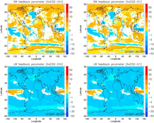
The spatial distribution of the ERF is analyzed by regressing in each model grid box the radiativefluxes at the TOA against the globally averagedΔT. Statistical significance of the results was checked by applying an unpaired two-tailed Student’s t test at the 5% significance level. The spatial distribution of the net (SW plus LW) ERF at the TOA from the GeoMIP median model presents positive values almost everywhere in both the 4xCO2
and Solar cases (Figure 2). There are a few small regions of statistically significant negative forcing that are probably related to cloud adjustments. They occur in cloudy regions of the eastern central Pacific and in high latitudes of the Northern Hemisphere for 4xCO2and are mostly limited to high latitudes in the Northern Hemisphere for Solar. The net ERF is more meridionally homogeneous for 4xCO2than for Solar, as the latter
Figure 1. Change in the global-mean net radiativefluxes at the TOA as a function of the global-mean change in surface temperature between experiments abrupt4xCO2and piControl (4xCO2, black) and between abrupt4xCO2and G1 (Solar, red) for the GeoMIP median model. The change in net (solid lines, asterisks), shortwave (dashed lines, triangles) and longwave (dotted lines, squares) all-sky radiativefluxes are shown as well as the shortwave and longwave clear-sky (dashed lines, triangles) and cloud-sky (dashed dotted lines, asterisks)fluxes. Symbols correspond to individual annual means over the 50 years of the simulations. Lines are bestfits to each set of points using the least squares method.
forcing follows the latitudinal distribution of insolation. Interestingly, the SW component of the ERF in 4xCO2
and the LW component of the ERF in Solar, which correspond largely to rapid adjustments, show some similarities in their pattern but with opposite sign in the Northern Hemisphere and up to midlatitudes in the Southern Hemisphere.
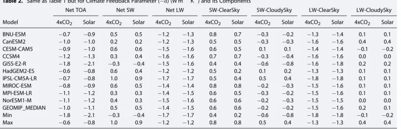
A negative feedback, as required for a stable system, is evident in all models for the netflux at the TOA for all-sky case (Figures 1 and S1). The GeoMIP median climate feedback for the Solar case is 1.1 ( 2.1 to 0.8) W m 2K 1 (Table 2). The regression lines associated with the netflux, as well as with the individual components are, in general, parallel between the 4xCO2and Solar cases indicating that the climate feedback is independent of the
forcing agent, which is in agreement with previous studies [e.g., Bala et al., 2010]. In both parts of the spectrum, the feedback is dominated by the clear-sky contribution, while clouds have a smaller additional impact on how climate reacts to the increase of CO2and/or increase in solar irradiance (Table 2). The SW clear-sky
component presents a positive feedback that arises because of a reduction in surface albedo due to the loss of sea ice and snow cover with increasing surface temperature, as well as increased absorption by increasing water vapor [Andrews et al., 2012a]. This positive feedback is compensated by a LW negative (stabilizing)
Figure 2. Spatial distribution of the (first row) effective net, (second row) shortwave, and (third row) longwave radiative forcing at the TOA associated with the abrupt4xCO2 piControl (4xCO2) and abrupt4xCO2 G1 (Solar) differences for the
GeoMIP median model. The white regions correspond to pixels where the difference is not statistically different from zero at the 5% level.
feedback parameter resulting from the combination of the blackbody, water vapor, and lapse-rate feedbacks [e.g., Soden and Held, 2006; Gregory and Webb, 2008]. Differences between clear- and cloudy-sky contributions are larger in the LW than in the SW. Moreover, there is compensation between the cloudy contributions in the SW and LW. We note that the models CESM-CAM5, IPSL-CM5A-LR, and HadGEM2-ES have a SW cloudy-sky feedback (or CRE feedback) parameter of opposite sign to the other GeoMIP models. Although the reasons for this have not been explored, it reflects the large diversity among models in terms of cloud feedbacks. Furthermore, the HadGEM2-ES is the only model to present an important difference in the SW clear-sky feedback between the 4xCO2and the Solar cases, with the former being larger than the latter (Table 2).
Andrews et al. [2012b] found that for increases in solar constant, a vegetation-dust feedback occurred not present when the model is forced with a quadrupling of CO2. In the solar forcing, an increase of bare soil
fraction in desert regions was observed resulting in additional dust in the atmosphere enhancing the reflection of SW radiation and reducing thereby the feedback parameter. This suggests that solar forcing cannot offset any feedbacks that are associated to CO2physiological/fertilization effects in Earth system models. However, the above mentioned vegetation-dust feedback does not seem to be included or play a significant role in the remaining GeoMIP models given the similarities between the feedback parameters of the 4xCO2and the Solar cases.
The spatial distribution of climate feedbacks was analyzed in the same way as for the forcing terms, i.e., each component Niat the TOA and surface was regressed against the globally averagedΔT at each model
grid box. As before, statistical significance of the results was checked by applying a Student’s t test at the 5% significance level. Despite the difference in the spatial distribution of the forcing between the 4xCO2
and the Solar cases (Figure 2), the SW and LW components of the climate feedback parameter present very similar, quasi-identical features for both forcing mechanisms (Figure 3). In the SW, negative feedbacks are mainly observed in cloudy regions over the oceans; whereas in the LW, the feedback is mostly negative everywhere, except in regions that become more moist and cloudier of the equatorial Pacific. The similarity in slope that was evident from Figure 1 therefore applies spatially. This holds even for the individual GeoMIP models used in the computation of the median model (Figures S3 and S4). There is indeed far more similarity between the climate feedback parameters for the two forcing mechanisms for a given model than between two different models for the same forcing mechanism. However, tofirst order, all models present the same main features as the GeoMIP median model (except for GISS-E2-R in the SW). The agreement in the spatial distribution of the feedback parameter between models is closer in the LW than in the SW case. For the latter, the regions with larger disagreement among models are in the Southern Ocean, the North Atlantic, and the equatorial Pacific. The disagreement in these cloudy regions highlights the diversity in how clouds respond to climate change in the different ESMs and point out the need to further understand cloud feedbacks, in particular, in the above mentioned regions.
Table 2. Same as Table 1 but for Climate Feedback Parameter ( α) (W m 2K ) and Its Componentsa
Net TOA Net SW Net LW SW-ClearSky SW-CloudySky LW-ClearSky LW-CloudySky
Model 4xCO2 Solar 4xCO2 Solar 4xCO2 Solar 4xCO2 Solar 4xCO2 Solar 4xCO2 Solar 4xCO2 Solar
BNU-ESM 0.7 0.9 0.5 0.5 1.2 1.3 0.8 0.7 0.3 0.2 1.3 1.4 0.1 0.1 CanESM2 1.0 1.0 0.2 0.2 1.2 1.3 0.5 0.5 0.3 0.3 1.6 1.6 0.4 0.4 CESM-CAM5 0.9 1.0 0.6 0.6 1.5 1.6 0.6 0.5 0.1 0.1 1.4 1.4 0.1 0.2 CCSM4 1.2 1.3 0.3 0.4 1.6 1.6 0.7 0.7 0.3 0.4 1.6 1.6 0.0 0.0 GISS-E2-R 1.8 2.1 0.3 0.4 1.5 1.6 0.4 0.4 0.6 0.8 1.6 1.8 0.2 0.2 HadGEM2-ES 0.6 0.8 0.6 0.4 1.2 1.2 0.5 0.2 0.1 0.2 1.3 1.3 0.1 0.1 IPSL-CM5A-LR 0.7 0.8 1.0 0.9 1.7 1.7 0.5 0.4 0.5 0.4 1.8 1.8 0.1 0.1 MIROC-ESM 0.8 0.9 0.6 0.5 1.4 1.4 0.8 0.8 0.2 0.3 1.5 1.6 0.1 0.1 MPI-ESM-LR 1.1 1.2 0.3 0.3 1.4 1.5 0.6 0.5 0.3 0.2 1.5 1.6 0.1 0.1 NorESM1-M 1.1 1.2 0.4 0.3 1.5 1.6 0.6 0.6 0.2 0.3 1.5 1.5 0.0 0.0 GEOMIP_MEDIAN 1.0 1.1 0.5 0.5 1.4 1.5 0.6 0.6 0.2 0.2 1.5 1.6 0.2 0.1 Min 1.8 2.1 0.3 0.4 1.7 1.7 0.4 0.2 0.6 0.8 1.8 1.8 0.1 0.2 Max 0.6 0.8 1.0 0.9 1.2 1.2 0.8 0.8 0.5 0.4 1.3 1.3 0.4 0.4
3.2. Surface Energy Fluxes
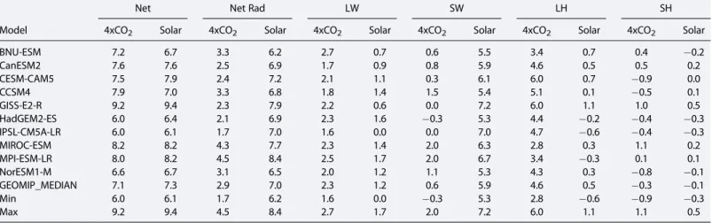
We now turn our analysis to surfacefluxes. The increase in CO2in 4xCO2and solar irradiance in Solar produce,
as expected, a positive ERF at the surface (Figures 4 and S5). However, the ERFS is much smaller in 4xCO2at 2.9 (1.7 to 4.5) W m 2than in Solar at 7.0 (6.2 to 8.4) W m 2(Table 3). The ERFS is dominated by the LW component in 4xCO2with a value of 2.3 (1.6 to 2.7) W m 2and the SW component in Solar with a value of
5.9 (5.3 to 7.2) W m 2. Both the LW component of the ERFS in 4xCO2and the SW component of the ERFS in
Solar are dominated by their clear-sky contributions. Interestingly, although the magnitudes are different, the patterns of the LW component of the ERFS bear some similarity between 4xCO2and Solar, which is not the
case for the SW component (Figure 5). This suggests that the LW component of the ERFS contains some rapid adjustments that are common to the two forcing mechanisms. A possible adjustment common to both forcings, and thus explaining the similarities in the spatial pattern, could be the rapid land warming. This will result in an increase of the outgoing LW radiation explaining the regions with negative LW ERFS.
Figure 4. Net energy (solid lines, asterisks) and net radiative (dashed lines, triangles)fluxes at the surface, shortwave (dotted lines, asterisks) and longwave (dashed lines, triangles) radiativefluxes at the surface, and nonradiative fluxes of latent heat (dotted lines, asterisks) and sensible heat (dashed lines, triangles) for both the abrupt4xCO2 piControl (4xCO2, black) and abrupt4xCO2 G1 (Solar, red) differences.
Figure 3. Climate feedback parameter (Wm-2K 1) for TOA shortwave and longwave radiation for the abrupt4xCO2 piControl (4xCO2) and abrupt4xCO2 G1 (Solar) differences.
The large difference in ERFS between the two mechanisms is largely compensated by opposing changes in nonradiative surface forcing terms. The atmosphere has a relatively small heat capacity so that all imbalances between the ERF at the TOA and at the surface need to be compensated by the nonradiative surface forcing terms to maintain tropospheric heat balance. The magnitudes and patterns of the LHF are very different between the two forcing mechanisms. As precipitation has to balance evaporation at the surface, this results in a rapid adjustment of the hydrological cycle that is different for the two forcing mechanisms. The large positive LHF (i.e., a reduction in evaporation) in the 4xCO2case is observed throughout most of the globe
(Figure 5). Yet regions with statistically significant negative LHF exist over bright surfaces such as ice-covered areas and desert regions and over the North Atlantic and Southern Ocean. There is a much smaller positive LHF in the Solar case. This initial stronger decrease in precipitation in the 4xCO2case is consistent with results
presented in previous works [e.g. Andrews et al., 2009; Bala et al., 2010; Schaller et al., 2013; Kravitz et al., 2013a]. This decrease in precipitation for an increase of CO2concentration has become increasingly well
understood and explains the decrease in precipitation in experiments where solar radiation management balances CO2radiative forcing [Andrews et al., 2009; Cao et al., 2011; O’Gorman et al., 2012; Schmidt et al., 2012;
Tilmes et al., 2013; Kravitz et al., 2013b; Schaller et al., 2013]. These works show that under a 4xCO2atmosphere, the climate responds by initially reducing the precipitation and then as surface temperature changes, the precipitation is increased with respect to preindustrial conditions. For a reduction in solar irradiance, the precipitation rates are reduced on a global scale compared to an atmosphere with 4xCO2. In agreement with
Tilmes et al. [2013], the magnitude and patterns of the SHF are fairly similar in the 4xCO2and Solar cases, suggesting again that the rapid adjustments are similar in the two experiments (Table 3 and Figure 5). The spatial distribution of the SHF shows mostly negative values over continents and positive values over the middle- and high-latitude oceans.
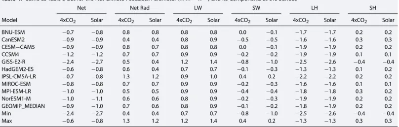
We now turn the analysis to the feedback parameters for the surface energy budget terms. For all terms of the surface energy budget, the regression lines for 4xCO2and Solar are almost parallel and consequently
their climate feedback parameters are equivalent. The feedback parameter for the LWflux is positive, i.e., it varies with the same sign as the globally averaged surface temperature, whereas for the SWflux, it is negative for most models (Figure 4 and Table 4). The positive feedback parameter in the LW is due to the warming and moistening of the atmosphere as the climate warms up in response to the forcing, thereby increasing the LW downwardflux more than the LW upward flux at the surface [Andrews et al., 2009]. Although all models agree on the sign of the LW feedback parameter at the surface, there is some diversity for that associated to the SWflux at the surface (Table 4 and Figure S5). The positive feedback parameter associated with the net radiativeflux at the surface is opposed by a negative feedback parameter for the latent heat flux (i.e., evaporation increases with surface temperature). Finally, the small slope of the SHflux indicates a corresponding small feedback in that component.
Table 3. Same as Table 1 but for the Effective Surface Forcing (W m 2) and the Effective Radiative Forcing at the Surface as Well as Its Components (W m 2) for the 4xCO2and the Solar Casesa
Net Net Rad LW SW LH SH
Model 4xCO2 Solar 4xCO2 Solar 4xCO2 Solar 4xCO2 Solar 4xCO2 Solar 4xCO2 Solar
BNU-ESM 7.2 6.7 3.3 6.2 2.7 0.7 0.6 5.5 3.4 0.7 0.4 0.2 CanESM2 7.6 7.6 2.5 6.9 1.7 0.9 0.8 5.9 4.6 0.5 0.5 0.2 CESM-CAM5 7.5 7.9 2.4 7.2 2.1 1.1 0.3 6.1 6.0 0.7 0.9 0.0 CCSM4 7.9 7.0 3.3 6.8 1.8 1.4 1.5 5.4 5.1 0.1 0.5 0.1 GISS-E2-R 9.2 9.4 2.3 7.9 2.2 0.6 0.0 7.2 6.0 1.1 1.0 0.5 HadGEM2-ES 6.0 6.4 2.1 6.9 2.3 1.6 0.3 5.3 4.4 0.2 0.4 0.3 IPSL-CM5A-LR 6.0 6.1 1.7 7.0 1.6 0.0 0.0 7.0 4.7 0.6 0.4 0.3 MIROC-ESM 8.2 8.2 4.3 7.7 2.3 1.4 2.0 6.3 2.8 0.3 1.1 0.2 MPI-ESM-LR 8.0 8.2 4.5 8.4 2.5 1.7 2.0 6.7 3.4 0.3 0.1 0.1 NorESM1-M 6.6 6.7 3.1 6.5 2.0 1.2 1.1 5.3 4.3 0.3 0.8 0.1 GEOMIP_MEDIAN 7.1 7.3 2.9 7.0 2.3 1.2 0.6 5.9 4.6 0.5 0.3 0.1 Min 6.0 6.1 1.7 6.2 1.6 0.0 0.3 5.3 2.8 0.6 0.9 0.3 Max 9.2 9.4 4.5 8.4 2.7 1.7 2.0 7.2 6.0 1.1 1.1 0.5
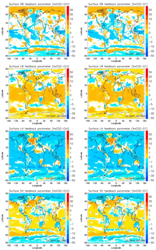
Although the forcings differ in mechanism and spatial distributions, the patterns of the two climate feedback parameters for the surface energy terms are quasi-identical for the 4xCO2and Solar cases in the GeoMIP
median model (Figure 6). The similarity in climate feedback parameters, not only in terms of global averages but also in their spatial distribution, is remarkable. This similarity is also observed in each one of the individual
Figure 5. Spatial distribution of (first row) net shortwave, (second row) net longwave, (third row) latent heat, and (fourth row) sen-sible heat effective surface forcing (W m 2) for the abrupt4xCO2 piControl (4xCO2) and abrupt4xCO2 G1 (Solar) differences.
Figure 6. Spatial distribution of net (first row) shortwave, (second row) longwave, (third row) latent heat, and (fourth row) sensible heat components of the climate feedback parameter at the surface for the abrupt4xCO2 piControl (4xCO2) and abrupt4xCO2 G1 (Solar) differences.
GeoMIP models used in the computation of the median model (Figures S7–S10) and points to a fundamental feature of the climate response.
4. Conclusions
Greenhouse gas forcing acts to trap heat in the atmosphere over the entire globe by day and by night with little meridional or seasonal variations, whereas the solar forcing acts only during the day and with a stronger meridional and seasonal dependence. While changes in CO2concentration perturb mainly the
LW radiation, changes in the solar irradiance act mainly on the SW.
An energetic perspective was used to investigate the rapid adjustments and feedbacks to solar and greenhouse gas forcing in 10 ESMs from the GeoMIP. Previous studies using the energy perspective to analyze the impact of solar forcing have focused on the netfluxes at the TOA and/or on the impact on the hydrological cycle. Here the different components of the energy budget, both at the TOA and the surface, were examined to better understand the impact of solar forcing in the context of idealized solar radiation management.
At the TOA, the ERF in Solar is dominated, as expected, by the SW clear-sky component, which is slightly compensated by a negative LW component, in particular, in the clear-sky. A cloudy-sky SW contribution of nearly 30% to the net SW ERF suggests a tropospheric adjustment in the cloud component to an increase in solar irradiance. In addition, model diversity in the spatial distribution of the SW feedback parameter in cloudy regions points to the uncertainty in the SW of how clouds feedback onto climate. Further understanding of cloud processes and how they impact climate, in particular, in the above mentioned regions, is therefore needed. However, all models agree in attributing a larger feedback to the clear-sky contributions for both forcings and in both parts of the spectrum. The largest contribution at the TOA in Solar in terms of feedbacks is from the SW and LW clear-sky components, which differ in sign: While the increase in solar irradiance induces a positive feedback in the SW, this is counteracted by a negative feedback in the LW. In 4xCO2, however, the
largest contribution comes from the SW cloudy-sky component and the LW clear-sky one, with both feedback parameters acting in the same direction.
The contributions to the ERF at the surface, namely the LW component in 4xCO2and the SW one in Solar,
are dominated by their clear-sky conditions. The energy imbalance between the TOA and the surface is compensated by a positive LHF (i.e., a reduction of evaporation) in 4xCO2as well as in Solar but with largely
different magnitude and spatial distribution and only a small SHF. The LHF is much smaller in the Solar case to compensate for a larger positive ERF at the surface. Similarities in the spatial pattern between both forcing mechanisms in the LW and the SHfluxes suggest that the rapid adjustments have some similarities in the two experiments. In addition, the SW feedback counteracts the amplifying feedback associated with the LW component. The resulting net radiative feedback at the surface is positive and is opposed by a negative (i.e., stabilizing) feedback from the latent heatflux (i.e., evaporation increases with surface temperature) while there is only a small feedback from the sensible heatflux.
Table 4. Same as Table 3 but for the Net Climate Feedback Parameter (W m 2K 1) and Its Components at the Surface
Net Net Rad LW SW LH SH
Model 4xCO2 Solar 4xCO2 Solar 4xCO2 Solar 4xCO2 Solar 4xCO2 Solar 4xCO2 Solar
BNU-ESM 0.7 0.8 0.8 0.8 0.8 0.8 0.0 0.1 1.7 1.7 0.2 0.2 CanESM2 0.9 0.9 0.4 0.4 0.8 0.9 0.5 0.5 1.6 1.6 0.3 0.3 CESM CAM5 0.9 0.9 0.8 0.7 0.8 0.8 0.0 0.1 1.9 1.9 0.2 0.2 CCSM4 1.2 1.2 0.7 0.7 0.9 0.9 0.2 0.2 1.9 1.9 0.1 0.1 GISS-E2-R 2.4 2.7 0.5 0.4 1.2 1.4 0.8 1.0 2.5 2.6 0.4 0.4 HadGEM2-ES 0.6 0.8 0.6 0.4 0.7 0.7 0.1 0.3 1.3 1.3 0.1 0.2 IPSL-CM5A-LR 0.7 0.8 1.3 1.2 0.9 1.0 0.4 0.2 2.2 2.2 0.2 0.2 MIROC-ESM 0.8 0.8 0.7 0.7 0.9 0.9 0.2 0.3 1.6 1.6 0.1 0.1 MPI-ESM-LR 1.0 1.0 0.5 0.5 0.9 0.9 0.4 0.4 1.8 1.8 0.3 0.2 NorESM1-M 1.0 1.1 0.6 0.6 0.8 0.9 0.2 0.3 1.9 1.9 0.2 0.2 GEOMIP_MEDIAN 0.9 1.0 0.7 0.6 0.8 0.9 0.1 0.2 1.8 1.9 0.2 0.2 Min 2.4 2.7 0.4 0.4 0.7 0.7 0.8 1.0 2.5 2.6 0.4 0.4 Max 0.6 0.8 1.3 1.2 1.2 1.4 0.4 0.2 1.3 1.3 0.3 0.3
The regression lines of the different components of the energy balance at the TOA and the surface are nearly parallel, indicating that feedback strengths remain constant regardless of the forcing mechanism acting on the climate system. This confirms previous studies [e.g., Andrews et al., 2009; O’Gorman et al., 2012], which have shown that the climate feedback was the same for different forcings in a global mean sense. Xie et al. [2013] suggest that aerosols and greenhouse gases exhibit similar responses over ocean based on similar regional patterns of ocean temperature and precipitation changes. Our results, however, reveal that the spatial distribution, both over land and ocean, of the climate feedback parameter is almost identical between the two forcing mechanisms analyzed in this work. This conclusion holds for each component of the energy budget at both the TOA and the surface. This equivalence is also exhibited by each one of the models used in the computation of the GeoMIP median model indicating that the climate feedback processes are largely independent of the forcing mechanism. This key result justifies further work to examine the mechanisms responsible for the quasi-identical spatial distribution of climate feedback parameters. In addition, it would be of interest to investigate if the strong similarity in climate feedback parameters holds for more
heterogeneous forcing associated to more realistic scenarios of possible implementation of geoengineering such as the GeoMIP experiment (G4) where aerosols are injected into the stratosphere at one point in the equator at a specific constant annual rate starting in the year 2020 [Kravitz et al., 2011].
References
Andrews, T. (2009), Forcing and response in simulated 20th and 21st century surface energy and precipitation trends, J. Geophys. Res., 114, D17110, doi:10.1029/2009JD011749.
Andrews, T., P. M. Forster, and J. M. Gregory (2009), A surface energy perspective on climate change, J. Clim., 22(10), 2557–2570, doi:10.1175/2008jcli2759.1.
Andrews, T., J. M. Gregory, P. M. Forster, and M. J. Webb (2012a), Cloud adjustment and its role in CO2radiative forcing and climate sensitivity:
A review, Surv. Geophys., 33(3-4), 619–635, doi:10.1007/s10712-011-9152-0.
Andrews, T., M. A. Ringer, M. Doutriaux-Boucher, M. J. Webb, and W. J. Collins (2012b), Sensitivity of an Earth system climate model to idealized radiative forcing, Geophys. Res. Lett., 39, L10702, doi:10.1029/2012GL051942.
Bala, G., K. Caldeira, and R. Nemani (2010), Fast versus slow response in climate change: Implications for the global hydrological cycle, Clim. Dyn., 35(2-3), 423–434, doi:10.1007/s00382-009-0583-y.
Bony, S., et al. (2006), How well do we understand and evaluate climate change feedback processes?, J. Clim., 19(15), 3445–3482, doi:10.1175/jcli3819.1. Caballero, R., and M. Huber (2013), State-dependent climate sensitivity in past warm climates and its implications for future climate
projections, Proc. Natl. Acad. Sci. U. S. A., 110(35), 14,162–14,167.
Cao, L., G. Bala, and K. Caldeira (2011), Why is there a short-term increase in global precipitation in response to diminished CO2forcing?,
Geophys. Res. Lett., 38, L06703, doi:10.1029/2011GL046713.
Colman, R. A., and B. J. McAvaney (2011), On tropospheric adjustment to forcing and climate feedbacks, Clim. Dyn., 36(9-10), 1649–1658, doi:10.1007/s00382-011-1067-4.
Doutriaux-Boucher, M., M. J. Webb, J. M. Gregory, and O. Boucher (2009), Carbon dioxide induced stomatal closure increases radiative forcing via a rapid reduction in low cloud, Geophys. Res. Lett., 36, L02703, doi:10.1029/2008GL036273.
Forster, P. M., T. Andrews, P. Good, J. M. Gregory, L. S. Jackson, and M. Zelinka (2013), Evaluating adjusted forcing and model spread for historical and future scenarios in the CMIP5 generation of climate models, J. Geophys. Res. Atmos., 118, 1139–1150, doi:10.1002/jgrd.50174. Gregory, J. M., and M. Webb (2008), Tropospheric adjustment induces a cloud component in CO2forcing, J. Clim., 21(1), 58–71,
doi:10.1175/2007jcli1834.1.
Gregory, J. M., W. J. Ingram, M. A. Palmer, G. S. Jones, P. A. Stott, R. B. Thorpe, J. A. Lowe, T. C. Johns, and K. D. Williams (2004), A new method for diagnosing radiative forcing and climate sensitivity, Geophys. Res. Lett., 31, L03205, doi:10.1029/2003GL018747.
Hansen, J., et al. (2005), Efficacy of climate forcings, J. Geophys. Res., 110, D18104, doi:10.1029/2005JD005776.
Kamae, Y., and M. Watanabe (2012), On the robustness of tropospheric adjustment in CMIP5 models, Geophys. Res. Lett., 39, L23808, doi:10.1029/2012GL054275.
Kamae, Y., and M. Watanabe (2013), Tropospheric adjustment to increasing CO2: Its timescale and the role of land-sea contrast, Clim. Dyn.,
41(11-12), 3007–3024, doi:10.1007/s00382-012-1555-1.
Kravitz, B., A. Robock, O. Boucher, H. Schmidt, K. E. Taylor, G. Stenchikov, and M. Schulz (2011), The Geoengineering Model Intercomparison Project (GeoMIP), Atmos. Sci. Lett., 12(2), 162–167, doi:10.1002/asl.316.
Kravitz, B., et al. (2013a), Climate model response from the Geoengineering Model Intercomparison Project (GeoMIP), J. Geophys. Res. Atmos., 118, 8320–8332, doi:10.1002/jgrd.50646.
Kravitz, B., et al. (2013b), An energetic perspective on hydrologic cycle changes in the Geoengineering Model Intercomparison Project (GeoMIP), J. Geophys. Res. Atmos., 118, 13,087–13,102, doi:10.1002/2013JD020502.
Lambert, F. H., and N. E. Faull (2007), Tropospheric adjustment: The response of two general circulation models to a change in insolation, Geophys. Res. Lett., 34, L03701, doi:10.1029/2006GL028124.
Meehl, G. A., W. M. Washington, T. M. L. Wigley, J. M. Arblaster, and A. Dai (2003), Solar and greenhouse gas forcing and climate response in the twentieth century, J. Clim., 16(3), 426–444, doi:10.1175/1520-0442(2003)016<0426:saggfa>2.0.co;2.
O’Gorman, P. A., R. P. Allan, M. P. Byrne, and M. Previdi (2012), Energetic constraints on precipitation under climate change, Surv. Geophys., 33(3-4), 585–608, doi:10.1007/s10712-011-9159-6.
Randall, D. A., et al. (2007), Climate models and their evaluation, in IPCC, 2007: Climate Change 2007: The Physical Science Basis. Contribution of Working Group I to the Fourth Assessment Report of the Intergovernmental Panel on Climate Change, edited by S. Solomon et al., Cambridge Univ. Press, Cambridge.
Schaller, N., J. Cermak, M. Wild, and R. Knutti (2013), The sensitivity of the modeled energy budget and hydrological cycle to CO2and solar
forcing, Earth Syst. Dyn., 4(2), 253–266, doi:10.5194/esd-4-253-2013.
Acknowledgments
We thank all participants of the Geoengineering Model Intercomparison Project and their model development teams, the CLIVAR/WCRP Working Group on Coupled Modeling for endorsing GeoMIP, and the scientists managing the Earth System Grid data nodes who have assisted with making GeoMIP output available. We further acknowledge the World Climate Research Programme’s Working Group on Coupled Modelling, which is responsible for CMIP, and we thank the climate modeling groups for producing and making available their model output. For CMIP, the U.S. Department of Energy’s Program for Climate Model Diagnosis and Intercomparison provides coordinating support and led development of software infrastructure in partnership with the Global Organization for Earth System Science Portals. This study was co-funded by the European Commission under the EU Seventh Research Framework Programme (grant agreement No. 283576, MACC II) and by the French Ministère de l’Ecologie, du Développement Durable, des Transports et du Logement (MEDDE) under the GMES-MDD program. This work was partly performed using HPC resources from GENCI-TGCC (grant 2013-t2013012201). Simulations performed by Ben Kravitz were supported by the NASA High-End Computing (HEC) Program through the NASA Center for Climate Simulation (NCCS) at Goddard Space Flight Center. Ben Kravitz is supported by the Fund for Innovative Climate and Energy Research (FICER). The Pacific Northwest National Laboratory is oper-ated for the U.S. Department of Energy by Battelle Memorial Institute under contract DE-AC05-76RL01830. Alan Robock is sup-ported by NSF grants AGS-1157525 and CBET-1240507. Andy Jones was supported by the Joint UK DECC/Defra Met Office Hadley Centre Climate Programme (GA01101). U. Niemeier and H. Schmidt have received funding from the European Commission’s Seventh Framework Programme through the IMPLICC project (FP7-ENV-2008-1-226567). K. Alterskjær and J.E. Kristjánsson received support from the European Union’s Seventh Framework Programme (FP7/2007–2013) under grant agreement 226567-IMPLICC, as well as from the Norwegian Research Council’s Programme for Supercomputing (NOTUR) through a grant of computing time. Helene Muri was supported by the European Commission under the EU Seventh Research Framework Programme (grant agreement 306395, EuTRACE). The CESM project (and therefore CCSM) is supported by the National Science Foundation and the Office of Science (BER) of the U.S. Department of Energy. The National Center for Atmospheric Research is funded by the National Science Foundation.
Schmidt, H., et al. (2012), Solar irradiance reduction to counteract radiative forcing from a quadrupling of CO2: Climate responses simulated
by four Earth system models, Earth Syst. Dyn., 3(1), 63–78, doi:10.5194/esd-3-63-2012.
Shine, K. P., J. Cook, E. J. Highwood, and M. M. Joshi (2003), An alternative to radiative forcing for estimating the relative importance of climate change mechanisms, Geophys. Res. Lett., 30(20), 2047, doi:10.1029/2003GL018141.
Soden, B. J., and I. M. Held (2006), An assessment of climate feedbacks in coupled ocean-atmosphere models, J. Clim., 19(14), 3354–3360, doi:10.1175/jcli3799.1.
Stowasser, M., K. Hamilton, and G. J. Boer (2006), Local and global climate feedbacks in models with differing climate sensitivities, J. Clim., 19(2), 193–209, doi:10.1175/jcli3613.1.
Taylor, K. E., R. J. Stouffer, and G. A. Meehl (2012), An overview of CMIP5 and the experiment design, Bull. Am. Meteorol. Soc., 93(4), 485–498, doi:10.1175/bams-d-11-00094.1.
Tilmes, S., et al. (2013), The hydrological impact of geoengineering in the Geoengineering Model Intercomparison Project (GeoMIP), J. Geophys. Res. Atmos., 118, 11,036–11,058, doi:10.1002/jgrd.50868.
Webb, M. J., et al. (2006), On the contribution of local feedback mechanisms to the range of climate sensitivity in two GCM ensembles, Clim. Dyn., 27(1), 17–38, doi:10.1007/s00382-006-0111-2.
Webb, M. J., F. H. Lambert, and J. M. Gregory (2013), Origins of differences in climate sensitivity, forcing and feedback in climate models, Clim. Dyn., 40(3-4), 677–707, doi:10.1007/s00382-012-1336-x.
Wyant, M. C., C. S. Bretherton, P. N. Blossey, and M. Khairoutdinov (2012), Fast cloud adjustment to increasing CO2in a superparameterized
climate model, J. Adv. Model. Earth Syst., 4(2), M05001, doi:10.1029/2011MS000092.
Xie, S.-P., B. Lu, and B. Xiang (2013), Similar spatial patterns of climate responses to aerosol and greenhouse gas changes, Nat. Geosci., 6, 828–832, doi:10.1038/ngeo1931.
Zelinka, M. D., S. A. Klein, K. E. Taylor, T. Andrews, M. J. Webb, J. M. Gregory, and P. M. Forster (2013), Contributions of different cloud types to feedbacks and rapid adjustments in CMIP5, J. Clim., 26(14), 5007–5027, doi:10.1175/jcli-d-12-00555.1.