HAL Id: hal-00243156
https://hal.archives-ouvertes.fr/hal-00243156v2
Submitted on 9 Jun 2008
HAL is a multi-disciplinary open access
archive for the deposit and dissemination of
sci-entific research documents, whether they are
pub-lished or not. The documents may come from
teaching and research institutions in France or
L’archive ouverte pluridisciplinaire HAL, est
destinée au dépôt et à la diffusion de documents
scientifiques de niveau recherche, publiés ou non,
émanant des établissements d’enseignement et de
recherche français ou étrangers, des laboratoires
Global sensitivity analysis of computer models with
functional inputs
Bertrand Iooss, Mathieu Ribatet
To cite this version:
Bertrand Iooss, Mathieu Ribatet. Global sensitivity analysis of computer models with functional
inputs.
Reliability Engineering and System Safety, Elsevier, 2009, 94 (7), pp.1194-1204.
�hal-00243156v2�
Global sensitivity analysis of computer models with
functional inputs
Bertrand IOOSS
∗and Mathieu RIBATET
†Submitted to: Reliability Engineering and System Safety
for the special SAMO 2007 issue
∗
CEA, DEN, DER/SESI/LCFR, F-13108 Saint-Paul-lez-Durance, France.
†
Ecole Polytechnique F´ed´erale de Lausanne, Chair of Statistics, STAT-IMA-FSB-EPFL,
´
Station 8, CH-1015 Lausanne, Switzerland.
Corresponding author: B. Iooss ; Email: [email protected]
Phone: +33 (0)4 42 25 72 73 ; Fax: +33 (0)4 42 25 24 08
Abstract
Global sensitivity analysis is used to quantify the influence of uncertain input parame-ters on the response variability of a numerical model. The common quantitative methods are appropriate with computer codes having scalar input variables. This paper aims at illustrating different variance-based sensitivity analysis techniques, based on the so-called Sobol’s indices, when some input variables are functional, such as stochastic processes or random spatial fields. In this work, we focus on large cpu time computer codes which need a preliminary metamodeling step before performing the sensitivity analysis. We propose the use of the joint modeling approach, i.e., modeling simultaneously the mean and the dispersion of the code outputs using two interlinked Generalized Linear Models (GLM) or Generalized Additive Models (GAM). The “mean model” allows to estimate the sensi-tivity indices of each scalar input variables, while the “dispersion model” allows to derive the total sensitivity index of the functional input variables. The proposed approach is compared to some classical sensitivity analysis methodologies on an analytical function. Lastly, the new methodology is applied to an industrial computer code that simulates the nuclear fuel irradiation.
Keywords: Sobol’s indices, joint modeling, generalized additive model, metamodel, stochastic process, uncertainty
1
INTRODUCTION
Modern computer codes that simulate physical phenomenas often take as inputs a high number of numerical parameters and physical variables, and return several outputs -scalars or functions. For the development and the use of such computer models, Sensitivity Analysis (SA) is an invaluable tool. The original technique, based on the derivative computations of the model outputs with respect to the model inputs, suffers from strong limitations for computer models simulating non-linear phenomena. More recent global SA techniques take into account the entire range of variation of the inputs and aim to apportion the whole output uncertainty to the input factor uncertainties (Saltelli et al. [21]). The global SA methods can also be used for model calibration, model validation, decision making process, i.e., any process where it is useful to know which are the variables that mostly contribute to the output variability.
The common quantitative methods are applicable to computer codes with scalar input variables. For example, in the nuclear engineering domain, global SA tools have been applied to numerous models where all the uncertain input parameters are modeled by random variables, possibly correlated - such as thermal-hydraulic system codes (Marqu`es et al. [13]), waste storage safety studies (Helton et al. [7]), environmental model of dose calculations (Iooss et al. [10]), reactor dosimetry processes (Jacques et al. [11]). Recent research papers have tried to consider more complex input variables in the global SA process, especially in petroleum and environmental studies:
• Tarantola et al. [27] work on an environmental assessment on soil models that use spatially distributed maps affected by random errors. This kind of uncertainty is modeled by a spatial random field (following a specified probability distribution), simulated at each code run. For the SA, the authors propose to replace the spatial input parameter by a “trigger” random parameter ξ that governs the random field simulation. For some values of ξ, the random field is simulated and for the other values, the random field values are put to zero. Therefore, the sensitivity index of ξ is used to quantify the influence of the spatial input parameter.
• Ruffo et al. [18] evaluate an oil reservoir production using a model that depends on different heterogeneous geological media scenarios. These scenarios, which are of limited number, are then substituted for a discrete factor (a scenario number) before performing the SA.
• Iooss et al. [9] study a groundwater radionuclide migration model which depend on several random scalar parameters and on a spatial random field (a geostatisti-cal simulation of the hydrogeologigeostatisti-cal layer heterogeneity). The authors propose to consider the spatial input parameter as an “uncontrollable” parameter. Therefore, they fit on a few simulation results of the computer model a double model, called a joint model: the first component models the effects of the scalar parameters while the second models the effects of the “uncontrollable” parameter.
In this paper, we tackle the problem of the global SA for numerical models and when some input parameters ε are functional. ε(u) is a one or multi-dimensional stochastic function where u can be spatial coordinates, time scale or any other physical parameters. Our work focuses on models that depend on scalar parameter vector X and involve some stochastic process simulations or random fields ε(u) as input parameters. The computer code output Y depends on the realizations of these random functions. These models are typically non linear with strong interactions between input parameters. Therefore, we concentrate our methodology on the variance based sensitivity indices estimation; that is, the so-called Sobol’s indices (Sobol [25], Saltelli et al. [21]).
To deal with this situation, a first natural approach consists in using either all the discretized values of the input functional parameter ε(u) or its decomposition into an appropriate basis of orthogonal functions. Then, for all the new scalar parameters related to ε(u), sensitivity indices are computed. However, in the case of complex functional parameters, this approach seems to be rapidly intractable as these parameters cannot be represented by a small number of scalar parameters (Tarantola et al. [27]). More-over, when dealing with non physical parameters (for example coefficients of orthogonal functions used in the decomposition), sensitivity indices interpretation may be laborious. Indeed, most often, physicists would prefer to obtain one global sensitivity index related to ε(u). Finally, a major drawback for the decomposition approach is related to the un-certainty modeling stage. More precisely, this approach needs to specify the probability density functions for the coefficients of the decomposition.
The following section presents three different strategies to compute the Sobol’s in-dices with functional inputs: (a) the macroparameter method, (b) the “trigger” parameter method and (c) the proposed joint modeling approach. Section 3 compares the relevance of these three strategies on an analytical example: the WN-Ishigami function. Lastly, the proposed approach is illustrated on an industrial computer code simulating fuel irradiation
in a nuclear reactor.
2
COMPUTATIONAL METHODS OF SOBOL’S
IN-DICES
First, let us recall some basic notions about Sobol’s indices. Let define the model
f : Rp
→ R
X 7→ Y = f (X)
(1)
where Y is the code output, X = (X1, . . . , Xp) are p independent inputs, and f is the
model function. f is considered as a “black box”, i.e. a function whose analytical formula-tion is unknown. The main idea of the variance-based SA methods is to evaluate how the variance of an input or a group of input parameters contributes to the output variance of f . These contributions are described using the following sensitivity indices:
Si =Var [E (Y |X i)]
Var(Y ) , Sij =
Var [E (Y |XiXj)]
Var(Y ) − Si− Sj, Sijk= . . . (2) These coefficients, namely the Sobol’s indices, can be used for any complex model functions f . The second order index Sij expresses the model sensitivity to the interaction between
the variables Xiand Xj(without the first order effects of Xiand Xj), and so on for higher
orders effects. The interpretation of these indices is natural as all indices lie in [0, 1] and their sum is equal to one. The larger an index value is, the greater is the importance of the variable or the group of variables related to this index.
For a model with p inputs, the number of Sobol’s indices is 2p − 1; leading to an
intractable number of indices as p increases. Thus, to express the overall output sensitivity to an input Xi, Homma & Saltelli [8] introduce the total sensitivity index:
STi = Si+ X j6=i Sij+ X j6=i,k6=i,j<k Sijk+ . . . = X l∈#i Sl (3)
where #i represents all the “non-ordered” subsets of indices containing index i. Thus, P
l∈#iSlis the sum of all the sensitivity indices having i in their index. The estimation
based on independent samples (Sobol [24], Saltelli [20]), or by refined sampling designs introduced to reduce the number of required model evaluations significantly, for instance FAST (Saltelli et al. [23]) and quasi-random designs (Saltelli et al. [22]).
Let us now consider a supplementary input parameter which is a functional input variable ε(u) ∈ R where u ∈ Rd is a d-dimensional location vector. ε(u) is defined by all
its marginal and joint probability distributions. In this work, it is supposed that random function realizations can be simulated. For example, these realizations can be produced using geostatistical simulations (Lantu´ejoul [12]) or stochastic processes simulations (Gen-tle [5]). Our model writes now
Y = f (X, ε) (4)
and in addition to the Sobol’s indices related to X, our goal is to derive methods to com-pute the sensitivity indices relative to ε, i.e., Sǫ (first order index), STε (total sensitivity
index), Siε(second order indices), Sijε, . . .
2.1
The macroparameter method
With the macroparameter method, the functional input parameter is not seen as a func-tional by the computer code. It is discretized in a potentially large number of values (for example several thousands), each of them being an input scalar parameter of the computer code. As all these values come from the functional input parameter (which pos-seses a specific correlation structure), they can be considered as an ensemble of correlated input parameters. Taking into account correlation between input variables in sensitivity analysis has been a challenging problem, recently solved by a few authors (see Da Veiga et al. [2] for a recent review).
One solution, proposed by Jacques et al. [11], to deal with correlated input parameters, is to consider multi-dimensional sensitivity indices (Sobol [25]): each group of correlated parameters is considered as a multi-dimensional parameter or macroparameter. One there-fore performs a sensitivity analysis by groups of correlated parameters. To estimate Sobol indices (first order, second order, . . . , total), a large number of input parameters (corre-lated and non corre(corre-lated) have to be generated. As we know how to generate independent samples of a correlated variables group, the simple Monte-Carlo sampling technique can be used (Sobol [24], Saltelli [20]). However, more efficient techniques than simple
Monte-Carlo (in terms of the required size sample), as FAST or quasi Monte-Monte-Carlo which use deterministic samples, are prohibited with correlated input variables.
In our context, this approach, using the simple Monte-Carlo algorithm, seems to be relevant as the input functional parameter ε(u) can be considered as a single multi-dimensional parameter (i.e. a macroparameter). For instance, the first order Sobol’s index related to ε(u) is defined as previously by
Sε=Var [E (Y |ε)]
Var(Y ) (5)
A simple way to estimate Sε= Dε/D is based on the Sobol [24] algorithm:
ˆ f0 = 1 N N X k=1 f (X(1)k , εk) (6a) ˆ D = 1 N − 1 N X k=1 f2(X(1)k , εk) − ˆf02 (6b) ˆ Dε = 1 N − 1 N X k=1 f (X(1)k , εk)f (X(2)k , εk) − ˆf02 (6c) where (X(1)k )k=1...N and (X (2)
k )k=1...N are two independent sets of N simulations of the
input vector X and (εk)k=1...N is a sample of N realizations of the random function ε(u).
To compute the sensitivity indices Si, the same algorithm is used with two independent
samples of (εk)k=1...N. In the same way, the total sensitivity index STε is derived from
the algorithm of Saltelli [20].
The major drawback of this method is that it may be cpu time consuming, mainly because of the sampling method. If d is the number of indices to be estimated, the cost of the Sobol’s algorithm is n = N (d + 1) while the cost of Saltelli’s algorithm to estimate d first order and d total sensitivity indices is n = N (d + 2). It is well known that, for complex computer models, an accurate estimation of Sobol’s indices by the simple Monte-Carlo method (independent random samples) requires N > 1000, i.e. more than thousand model evaluations for one input parameter (Saltelli et al. [22]). In complex industrial applications, this approach is intractable due to the cpu time cost of one model evaluation and the possible large number of input parameters.
2.2
The “trigger” parameter method
Dealing with spatially distributed input variables, Tarantola et al. [27] propose an alter-native that uses an additional scalar input parameter ξ - called the “trigger” parameter. ξ ∼ U [0, 1] governs the random function simulation. More precisely, for each simulation, if ξ < 0.5, the functional parameter ε(u) is fixed to a nominal value ε0(u) (for example
the mean E[ε(u)]), while if ξ > 0.5, the functional parameter ε(u) is simulated. Using this methodology, it is possible to estimate how sensitive the model output is to the presence of the random function. Tarantola et al. [27] use the Extended FAST method to com-pute the first order and total sensitivity indices of 6 scalar input factors and 2 additional “trigger” parameters. For their study, the sensitivity indices according to the “trigger” pa-rameters are small and the authors conclude that it is unnecessary to model these spatial errors more accurately.
Contrary to the previous method, there is no restriction about the sensitivity indices estimation procedure - i.e. Monte-Carlo, FAST, quasi Monte-Carlo. However, there are two major drawbacks for this approach:
• As the macroparameter method, it also requires the use of the computer model to perform the SA and it may be problematic for large cpu time computer models. This problem can be compensated by the use of an efficient quasi Monte-Carlo algorithm for which the sampling design size can be decreased to N = 100.
• As underlined by Tarantola et al. [27], ξ reflects only the presence or the absence of the stochastic errors on ε0(u). Therefore, the term Var[E(Y |ξ)] does not quantify
the contribution of the random function variability to the output variability Var(Y ). We will discuss about the significance of Var[E(Y |ξ)] later, during our analytical function application.
2.3
The joint modeling approach
To perform a variance-based SA for time consuming computer models, some authors pro-pose to approximate the computer code, starting from an initial small-size sampling design, by a mathematical function often called response surface or metamodel (Marseguerra et al. [14], Volkova et al. [28], Fang et al. [3]). This metamodel, requiring negligible cpu time, is then used to estimate Sobol’s indices by any method, for example the simple Monte-Carlo algorithm. For metamodels with sufficient prediction capabilities, the bias between the
exact Sobol’s indices (from the computer code) and the Sobol’s indices estimated via the metamodel is negligible. Indeed, it has been shown that the unexplained variance part of the computer code by the metamodel (which can be measured) corresponds to this bias (Sobol [26]). Several choices of metamodel can be found in the literature: polynomials, splines, Gaussian processes, neural networks, . . . The fitting process is often based on least squares regression techniques. Thus, for the functional input problem, one strategy may be to fit a metamodel with a multi-dimensional scalar parameters representing ε(u) as an input parameter - i.e. its discretization or its decomposition into an appropriate basis. This process would correspond to a metamodeling approach for the macroparame-ter method. However, this approach seems to be impracticable due to the potential large number of scalar parameters: applying regression techniques supposes to have more obser-vation points (simulation sets) than input parameters and important numerical problem (like matrix conditioning) might occur while dealing with correlated input parameters.
A second option is to substitute each random function realization for a discrete number, which can correspond to the scenario parameter of Ruffo et al. [18] (where the number of geostatistical realizations is finite and fixed, and where each different value of the discrete parameter corresponds to a different realization). Then, a metamodel is fitted using this dicrete parameter as a qualitative input variable. However, using a metamodel is interesting when only a few runs of the code is available, which correponds to a more limited number of realizations of the functional input. This restriction of the possible realizations of the input random function to a few ones is not appropriate in a general context.
Another strategy considers ε(u) as an uncontrollable parameter. A metamodel is fitted in function of the other scalar parameters X:
Ym(X) = E(Y |X) (7)
Therefore, using the relation
Var(Y ) = Var[E(Y |X)] + E[Var(Y |X)] (8) it can be easily shown that the sensitivity indices of Y given the scalar parameters X =
(Xi)i=1...p write (Iooss et al. [9]) Si=Var[E(Y m|Xi)] Var(Y ) , Sij= Var[E(Ym|XiXj)] Var(Y ) − Si− Sj, . . . (9) and can be computed by classical Monte-Carlo techniques applied on the metamodel Ym. Therefore, using equation (8), the total sensitivity index of Y according to ε(u)
corresponds to the expectation of the unexplained part of Var(Y ) by the metamodel Ym:
STε =E[Var(Y |X)]
Var(Y ) (10)
Using this approach, our objective is altered because it is impossible to decompose the ε effects into an elementary effect (Sε) as well as the interaction effects between ε and
the scalar parameters (Xi)i=1...p. However, we see below that our technique allows a
qualitative appraisal of the interaction indices.
The sensitivity index estimations from equations (9) and (10) raise two difficulties: 1. It is well known that classical parametric metamodels (based on least squares fitting)
are not adapted to estimate E(Y |X) accurately due to the presence of heteroscedas-ticity (induced by the effect of ε). Such cases are analyzed by Iooss et al. [9]. The authors show that heteroscedasticity may lead to sensitivity indices misspecifica-tions.
2. Classical non parametric methods, such as Generalized Additive Models (Hastie and Tibshirani [6]) and Gaussian processes (Sacks et al. [19]) that can provide efficient estimation of E(Y |X) (examples are given in Iooss et al. [9]), even in high dimensional input cases (p > 5). However, these approaches are based on a homoscedasticity hypothesis and do not enable the estimation of Var(Y |X). To solve the second problem, Zabalza-Mezghani et al. [30] propose the use of a theory developed for experimental data (McCullagh and Nelder [15]): the simultaneous fitting of the mean and the dispersion by two interlinked Generalized Linear Models (GLM), which is called the joint modeling (see Appendix A.1). Besides, to resolve the first problem, this approach has been extended by Iooss et al. [9] to non parametric models. This generalization allows more complexity and flexibility. The authors propose the use of Generalized Additive Models (GAMs) based on penalized smoothing splines (Wood [29]). A succint description of GAM and joint GAM is given in Appendix A.2. GAMs allow
model and variable selections using quasi-likelihood function, statistical tests on coeffi-cients and graphical display. However, compared to other complex metamodels, GAMs impose an additive effects hypothesis. Therefore, two metamodels are obtained: one for the mean component Ym(X) = E(Y |X); and the other one for the dispersion component
Yd(X) = Var(Y |X). The sensitivity indices of X are computed using Ym with the
stan-dard procedure (Eq. (9)), while the total sensitivity index of ε(u) is computed from E(Yd)
(Eq. (10)). Using the model for Yd as well as the associated regression diagnostics, it is
possible to deduce qualitative sensitivity indices for the interactions between ε(u) and the scalar parameters of X.
One major assumption of the joint modeling approach is that the “mean response” of the computer code is well handled using Ym. Consequently, all the unexplained part of
the computer model by this metamodel is due to the uncontrollable parameter. In other words, the better the mean component metamodel is, the smaller is the influence of the uncontrollable parameter. This is a strong assumption which has to be validated in order to avoid erroneous results. In fact, some simple statistical and graphical tools can be used while fitting the mean component (Iooss et al. [9]): the explained deviance value, the observed responses versus predicted values plot (and its quantile-quantile plot) and the deviance residuals plot. This last plot allows to detect some fitting problems by revealing possible biases or large residual values. Some examples are given in section 3.2. These tools can also be applied for the dispersion component fit. For a detailed overview of these diagnostic tools, one can refer to McCullagh & Nelder [15].
3
APPLICATION TO AN ANALYTICAL EXAMPLE
The three previously proposed methods are first illustrated on a simple analytical model with two scalar input variables and one functional input:
Y = f (X1, X2, ε(t)) = sin(X1) + 7 sin(X2)2+ 0.1[max t (ε(t))]
4sin(X
1) (11)
where Xi ∼ U[−π; π] for i = 1, 2 and ε(t) is a white noise, i.e. an i.i.d. stochastic
pro-cess ε(t) ∼ N (0, 1). In our model simulations, ε(t) is discretized in one hundred values: t = 1 . . . 100. The function (11) is similar to the well-known Ishigami function (Homma and Saltelli [8]) but substitute the third parameter for the maximum of a stochastic
pro-cess. Consequently, we call our function the white-noise Ishigami function (WN-Ishigami). Although the WN-Ishigami function is an analytical model, the introduction of the maxi-mum of a stochastic process inside a model is quite realistic. For example, some computer models simulating physical phenomena can use the maximum of time-dependent variable - river height, rainfall quantity, temperature. Such input variable can be modeled by a temporal stochastic process.
As for the Ishigami function, we can immediately deduce from the formula (11):
Sε= S12= S2ε= S12ε= 0 (12)
Then, we have
ST1 = S1+ S1ε, ST2 = S2, STε = S1ε (13)
In the following, we focus our attention on the estimation of S1, S2and STε.
Because of a particularly complex probability distribution of the maximum of a white noise, there is no analytical solution for the theoretical Sobol’s indices S1, S2 and STε for
the WN-Ishigami function. Even with the asymptotic hypothesis (number of time steps tending to infinity), where the maximum of the white noise follows Generalized Extreme Value distribution, theoretical indices are unreachable. Therefore, our benchmark Sobol’s indices values are derived from the Monte-Carlo method.
3.1
The macroparameter and “trigger” parameter methods
Table 1 contains the Sobol’s index estimates using the macroparameter and “trigger” parameter methods. As explained before, we can only use some algorithms based on independent Monte-Carlo samples. We apply the algorithm of Sobol [24] that computes S1, S2, S1εat a cost n = 4N and the algorithm of Saltelli [20] which computes the first
order indices S1, S2and the total sensitivity indices ST1, ST2, STε at a cost n = 5N (where
N is the size of the Monte-Carlo samples, cf. section 2.1). For the estimation, the size of the Monte-Carlo samples is limited to N = 10000 because of memory computer limit. Indeed, the functional input ε(u) contains for each simulation set 100 values. Then, the input sample matrix has the dimension N × 102 which becomes extremely large when N increases. To evaluate the effect of this limited Monte-Carlo sample size N , each Sobol’s index estimate is associated to a standard-deviation estimated by bootstrap (Saltelli et al.
[22]) - with 100 replicates of the input-output sample. The obtained standard-deviations (sd) are relatively small, of the order of 0.01, which is rather sufficient for our exercise.
Remark: We have also tried to estimate Sobol’s indices with smaller Monte-Carlo sample sizes N . The order of the obtained standard-deviations (estimated by bootstrap) of the Sobol’s estimates are the following: sd ∼ 0.02 for N = 5000, sd ∼ 0.04 for N = 1000 and sd ∼ 0.06 for N = 500. We conclude that the Monte-Carlo estimates are sufficiently accurate for N > 5000.
[Table 1 about here.]
Macroparameter
For the macroparameter method, the theoretical relations between indices given in (13) are satisfied. We are therefore confident with the estimates obtained with this method and we choose the Sobol’s indices obtained with Saltelli’s algorithm as the reference indices:
S1= 55.1%, S2= 20.7%, STε = 24.8%
The Sε, S12, S2ε and S12εindices (Eq. (12)) are not reported in table 1 as estimates are
negligible.
Trigger parameter
Using the “trigger” parameter method, the estimates reported in table 1 are quite far from the reference values. The inadequacies are larger than 30% for all the indices, and can be larger than 60% for a few ones (S2and ST2). Moreover, the relations given in (13)
are not satisfied at all. Actually, replacing the input parameter ε(u) by ξ which governs the presence or the absence of the functional input parameter changes the model. When ε is not simulated, it is replaced by its mean (zero) and the WN-Ishigami function becomes Y = sin(X1) + 7 sin(X2)2. Therefore, the mix of the WN-Ishigami model and this new
model perturbs the estimation of the sensitivity indices, even those unrelated to ε (like X2). In conclusion, the obtained results are in concordance with the expected results.
This result confirms our expectation: sensitivity indices derived from the “trigger” parameter method have not the same sense that the classical ones, i.e., the measure of the contribution of the input parameter variability to the output variable variability. The sensitivity indices obtained with these two methods are unconnected because the “trigger”
parameter method changes the structure of the model.
3.2
The joint modeling approach
We apply now the joint modeling approach which requires an initial input-output sample to fit the joint metamodel - the mean component Ym and the dispersion component Yd.
For our application, a learning sample size of n = 500 was considered; i.e., n independent random samples of (X1, X2, ε(u)) were simulated leading to n observations for Y . Joint
GLM and joint GAM fitting procedures are fully described in Iooss et al. [9]. Some graphical residual analyses are particularly useful to check the relevance of the mean and dispersion components of the joint models. In the following, we give the results of the joint models fitting on a learning sample (X1, X2, ε(u), Y ). Let us recall that we fit a
model to predict Y in function of (X1, X2).
Joint GLM fitting
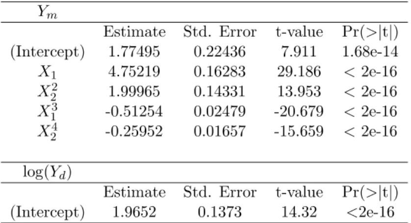
For the joint GLM, a fourth order polynomial for the parametric form of the model is considered. Moreover, only the explanatory terms are retained in our regression model using analysis of deviance and the Fisher statistics. The equation of the mean component writes:
Ym= 1.77 + 4.75X1+ 1.99X22− 0.51X13− 0.26X24. (14)
The value estimates, standard-deviation estimates and Student test results on the regres-sion coefficients are given in table 2. Residuals graphical analysis makes it also possible to appreciate the model goodness-of-fit.
[Table 2 about here.]
The explained deviance of this model is Dexpl = 73%. It can be seen that it remains
27% of non explained deviance due to the model inadequacy and/or to the functional input parameter. The predictivity coefficient, i.e. coefficient of determination R2computed on
a test sample, is Q2= 70%. Q2 is relatively coherent with the explained deviance.
For the dispersion component, using analysis of deviance techniques, none significant explanatory variable were found: the heteroscedastic pattern of the data has not been retrieved. Thus, the dispersion component is supposed to be constant (see Table 2);
and the joint GLM model is equivalent to a simple GLM - but with a different fitting procedure.
Joint GAM fitting
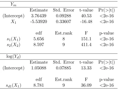
At present, we try to model the data using a joint GAM. For each component (mean and dispersion), Student test for the parametric part and Fisher statistics for the non parametric part allow us to keep only the explanatory terms (see Table 3). The resulting model is described by the following features:
Ym = 3.76 − 5.54X1+ s1(X1) + s2(X2) ,
log(Yd) = 1.05 + sd1(X1) ,
(15)
where s1(·), s2(·) and sd1(·) denote three penalized spline smoothing terms.
[Table 3 about here.]
The explained deviance of the mean component is Dexpl = 92% and the
predictiv-ity coefficient is Q2 = 77%. Therefore, the joint GAM approach outperforms the joint
GLM one. Indeed, the proportion of explained deviance is clearly greater for the GAM model. Even if this is obviously related to an increasing number of parameters; this is also explained as GAMs are more flexible than GLMs. This is confirmed by the increase of the predictivity coefficient - from 70% to 77%. Moreover, due to the GAMs flexibility, the explanatory variable X1 is identified for the dispersion component. The interaction
between X1and the functional input parameter ε(u) which governs the heteroscedasticity
of this model is therefore retrieved.
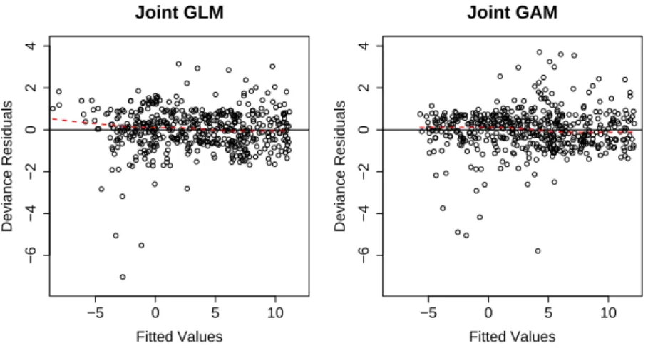
Figure 1 shows that the deviance residuals for the mean component of the joint GAM seem to be more homogeneously dispersed around the x-axis than the deviance residuals of the joint GLM. This leads to a better prediction from the joint GAM on the whole range of the observations.
[Figure 1 about here.]
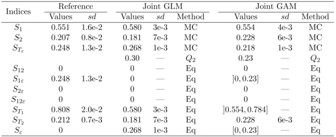
Sobol’s indices
From the joint GLM and the joint GAM, Sobol’s sensitivity indices can be computed using equations (9) and (10) - see Table 4. The reference values are extracted from the results of the macroparameter method via Saltelli’s algorithm (see Table 1) and from the
WN-Ishigami analytical form (11) (for example we know that S12 = 0 because there is
no interaction between X1and X2). The standard deviation estimates (sd) are obtained
from 100 replicates of the Monte-Carlo estimation procedure - which uses N = 10000 for the size of the Monte-Carlo samples (see section 2.1). The joint GLM and joint GAM give approximately good estimates of S1and S2. Despite the joint GLM leads to an acceptable
estimation for STε, we will see later that it is fortuitous. The estimation of STε with
the joint GAM seems also satisfactory but not accurate. In fact, an efficient modeling of Var(Y |X) is difficult, which is a common statistical difficulty in heteroscedastic regression problems (Antoniadis & Lavergne [1]).
Another way to estimate the total sensitivity index STε is to compute the unexplained
variance of the mean component model given directly by 1 − Q2, where Q2 is the
pre-dictivity coefficient of the mean component model. In practical applications, Q2 can be
estimated using leave-one-out or cross validation procedures. In our analytical case, the index is estimated with the former method and leads to a correct estimation - 0.23 instead of 0.25.
[Table 4 about here.]
For the other sensitivity indices, the conclusions draw from the GLM formula are completely erroneous. As the dispersion component is constant, Sε= STε = 0.268 while
Sε = 0 in reality. In contrary, the deductions draw from GAM formulas are exact:
(X1, ε) interaction sensitivity is strictly positive (S1ε > 0) because X1 is active in the
dispersion component Yd, S2ε = S12ε = 0, ST2 = S2 and S12 = S23 = S123 = 0. The
drawback of this method is that some indices (S1ε, Sε and ST1) remain unknown due to
the non separability of the dispersion component effects. However, we can easily deduce some variation intervals which contain these indices: Sε and S1ε are smaller than STε
while S1+ min(S1ε) ≤ ST1 ≤ S1+ max(S1ε). All these additional information provide
qualitative importance measures for the unknown indices.
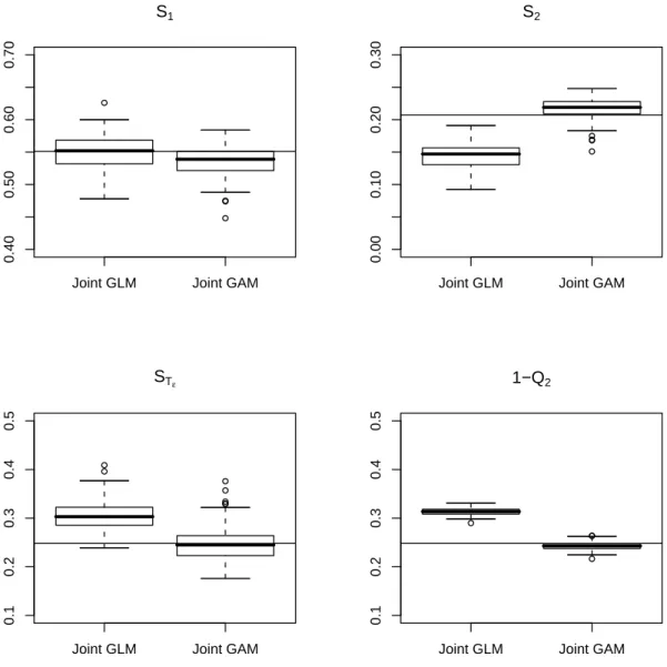
By estimating Sobol’s indices with those obtained from other learning samples, we observe that the estimates are rather dispersed: it seems that the estimates are not robust according to different learning samples for the joint models. To examine this effect, we propose to study two different sample sizes (n = 200 and n = 500). For each sample size, the distribution of the Sobol’s indices estimates is assessed using a bootstrap procedure. Figures 2 and 3 show the results of this investigation, which are particularly convincing.
Several conclusion can be drawn:
• For the joint GAM, the boxplot interquartile interval of each index contains its reference value. In contrary, the joint GLM fails to obtain correct estimates: except for S1, the sensitivity reference values are outside the interquartile intervals of the
obtained boxplots.
• The superiority of the joint GAM with respect to the joint GLM is corroborated, especially for S2and STε.
• The increase of the learning sample size has no effect on the joint GLM results (due to the parametric form of this model). However, for the joint GAM, boxplots widths are strongly reduced from n = 200 to n = 500. In addition, the mean estimates seem to converge to the reference values.
• As explained before, the estimation of STε using the predictivity coefficient Q2 is
markedly better than through the dispersion component model. This is not the case for the joint GLM. Moreover, we confirm that the previous result of table 4, STε = 0.268, was a good case: with 100 replicates, STε ranges from 0.24 to 0.35
(Figure 3).
[Figure 2 about here.] [Figure 3 about here.]
In conclusion, this example shows that the joint models, and specially the joint GAM, can adjust rather complex heteroscedastic situations. Of course, additional tests are needed to confirm this result. Moreover, the joint models offer a theoretical basis to compute efficiently global sensitivity indices for models with functional input parame-ter. Finally, the required number of computer model evaluations is much smaller with the joint modeling method (here n = 200 or n = 500 gives good results with the joint GAM) compared to the one of Monte-Carlo based techniques. For exemple, using the macroparameter method (cf. section 3.1) and taking N = 5000, we need to compute n = 25000 model evaluations to estimate first order and total sensitivity indices (via Saltelli’s algorithm).
4
APPLICATION TO A NUCLEAR FUEL
IRRADI-ATION SIMULIRRADI-ATION
The METEOR computer code, developed within the Fuel Studies Department in CEA Cadarache, studies the thermo-mechanical behavior of the fuel rods under irradiation in a nuclear reactor core. In particular, it computes the fission gas swelling and the cladding creep (Garcia et al. [4]). These two output variables are considered in our analysis. These variables are of fundamental importance for the physical understanding of the fuel behavior and for the monitoring of the nuclear reactor core.
Input parameters of such mechanical models can be evaluated either by database analy-ses, arguments invoking simplifying hypotheanaly-ses, expert judgment. All these considerations lead to assign to each input parameter a nominal value associated with an uncertainty. In this study, six uncertain input parameters are considered: the initial internal pressure X1, the pellet and cladding radius X2, X3, the microstructural fuel grain diameter X4,
the fuel porosity X5 and the time-dependent irradiation power P (t). X1, . . . , X5 are
all modeled by Gaussian independent random variables with the following coefficient of variations: cv(X1) = 0.019, cv(X2) = 1.22 × 10⁻³, cv(X3) = 1.05 × 10⁻³, cv(X4) = 0.044,
cv(X5) = 0.25. The last variable P (t) is a temporal function (discretized in 3558 values)
and its uncertainty ε(t) is modelled like a stochastic process. For simplicity, an Additive White Noise (AWN), of uniform law ranging between −5% and +5%, was introduced.
As in the previous application, additionally to its scalar random variables, the model includes an input functional variable P (t). To compute Sobol’s indices of this model, we have first tried to use the macroparameter method. We have succedeed to perform the calculations with N = 1000 (for the Monte-Carlo sample sizes of Eqs. (6a), (6b) and (6c)). The sensitivity indices estimates have been obtained after 10 computation days and were extremely imprecise, with strong variations between 0 and 1. Because of the required cpu time, an increase of the sample size N to obtain acceptable sensitivity estimates was unconceivable. Therefore, the goal of this section is to show how the use of the joint modeling approach allows to estimate the sensitivity indices of the METEOR model and, in particular, to quantify the functional input variable influence.
500 METEOR calculations were carried out using Monte-Carlo sampling of the input parameters (using Latin Hypercube Sampling). As expected, the AWN on P (t) generates an increase in the standard deviation of the output variables (compared to simulations
without a white noise): 6% increase for the variable fission gas swelling and 60% for the variable cladding creep.
4.1
Gas swelling
We start by studying the gas swelling model output. With a joint GLM, the following result for Ym and Yd were obtained:
Ym = −76 − 0.4X1+ 20X2+ 8X4+ 134X5+ 0.02X42− 2X2X4− 6X4X5 log(Yd) = −2.4X1 (16)
The explained deviance of the mean component is Dexpl= 86%. As the residual analyses
of mean and dispersion components do not show any biases, the resulting model seems satisfactory. The joint GAM was also fitted on these data and led to similar results. Thus, it seems that spline terms are useless and that a joint GLM model is appropriate.
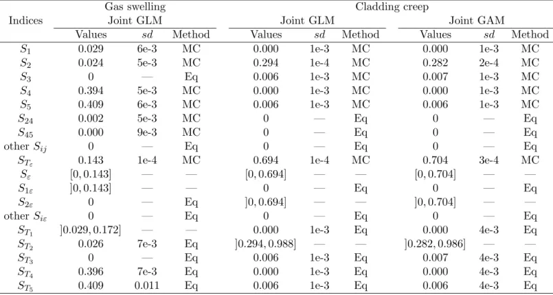
Table 5 shows the results for the Sobol’s indices estimation using Monte-Carlo methods applied on the metamodel (16). The standard deviation (sd) estimates are obtained from 100 replicates of the Monte-Carlo estimation procedure -which uses 105 model
computa-tions for one index estimation. It is useless to perform the Monte-Carlo estimation for some indices because they can be deduced from the joint model equations. For example, S3 = 0 (resp. Sε2 = 0) because X3 (res. X2) is not involved in the mean (resp.
dis-persion) component in equation (16). Moreover, we know that S1ε> 0 because X1 is an
explanatory variable inside the dispersion component Yd. However, this formulation does
not allow to have any idea about Sǫ which reflects the first order effect of ε. Therefore,
some indices are not accessible, such as Sε and S1ε non distinguishable inside the total
sensitivity index STε. Finally, we can check that 5 X i=1 Si+ 5 X i,j=1,i<j Sij+ STε = 1 holds -up to numerical approximations.
It can be seen that X4(grain diameter) and X5 (fuel porosity) are the most influent
factors (each one having 40% of influence), and do not interact with the irradiation power P (t) (represented by its uncertainty ε). In addition, the effect of P (t) is not negligible (STε = 14%) and parameter X1 (internal pressure) acts mainly with its interaction with
P (t). A sensitivity analysis by fixing X1could allow us to obtain some information about
4.2
Cladding creep
We study now the cladding creep model output. With a joint GLM, the model for Ym
and Yd is: Ym = −2.75 + 1.05X2− 0.15X3− 0.58X5 log(Yd) = 156052 − 76184X2+ 9298X22 (17)
The explained deviance of the mean component is Dexpl= 26%. As the residual analyses of
mean and dispersion components show some biases, the resulting model is not satisfactory. For the joint GAM, the spline terms {s(X2), s(X3), s(X5)} and s(X2) are added within
the mean component and the dispersion component respectively. The explained deviance of the mean component is Dexpl = 29% which is not significantly greater than 26%.
However, as the mean component residual biases of the joint GAM are smaller than those observed for the joint GLM, the joint GAM seems to be more relevant than the joint GLM.
Table 5 shows the Sobol’s index estimates using Monte-Carlo methods and deductions from the joint model equations. For the joint GLM and joint GAM of the cladding creep,
5 X i=1 Si+ 5 X i,j=1,i<j
Sij+ STε = 1 holds – up to numerical imprecisions. Due to the proximity
of the two joint models, results are similar. This analysis shows that the parameter X2
(pellet radius) explains 28% of the uncertainty of the cladding creep phenomenon, while the other scalar parameters have negligible influence. The greater part of the cladding creep variance (STε= 70%) is explained by the irradiation power uncertainty (the AWN).
Physicists may be interested in quantifying the interaction influence between the pellet radius and the irradiation power. Unfortunately, this interaction is not available for the moment in our analysis.
[Table 5 about here.]
5
CONCLUSION
This paper has proposed a solution to perform global sensitivity analysis for time consum-ing computer models which depend on functional input parameters, such as a stochastic process or a random field. Our purpose concerned the computation of variance-based im-portance measures of the model output according to the uncertain input parameters. We
have discussed a first natural solution which consists in integrating the functional input parameter inside a macroparameter, and using standard Monte-Carlo algorithms to com-pute sensitivity indices. This solution is not applicable for time consuming comcom-puter code. We have discussed another solution, used in previous studies, based on the replacement of the functional input parameter by a “trigger” parameter that governs the integration or not of the functional input uncertainties. However, the estimated sensitivity indices are not the expected ones due to changes in the model structure carrying out by the method itself. Finally, we have proposed an innovative strategy, the joint modeling method, based on a preliminary step of double (and joint) metamodel fitting, which resolves the large cpu time problem of Monte-Carlo methods. It consists in rejecting the functional input parameters in noisy input variables. Then, two metamodels depending only on the scalar random input variables are simultaneously fitted: one for the mean function and one for the dispersion (variance) function.
Tests on an analytical function have shown the relevance of the joint modeling method, which provides all the sensitivity indices of the scalar input parameters and the total sensitivity index of the functional input parameter. In addition, it reveals in a qualitative way the influential interactions between the functional parameter and the scalar input parameters. It would be interesting in the future to be able to distinguish the contributions of several functional input parameters that are currently totally mixed in one sensitivity index. This is the main drawback of the proposed method in its present form.
In an industrial application, the usefulness and feasibility of our methodology has been established. Indeed, other methods are not applicable in this application because of large cpu time of the computer code. To a better understanding of the model behavior, the information brought by the global sensitivity analysis can be very useful to the physicist or the modeling engineer. The joint model can also be useful to propagate uncertainties in complex models, containing input random functions, to obtain some mean predictions with their confidence intervals.
6
ACKNOWLEDGMENTS
This work was supported by the “Simulation” program managed by the CEA/Nuclear Energy Division. We are grateful to P. Obry (CEA Cadarache/D´epartement d’Etude des Combustibles) for the authorization to use the METEOR application. All the statistical
parts of this work have been performed within the R environment and the “sensitivity” and “JointModeling” packages. We are grateful to the referees whose comments significantly helped to improve the paper.
APPENDIX A: JOINT MODELING OF MEAN AND
DISPERSION
A.1 Joint Generalized Linear Models
GLMs allow to extend traditional linear models by the use of a distribution which belongs to the exponential family and a link function that connects the explanatory variables to the explained variable (Nelder & Wedderburn [17]). The joint GLM consists in putting a GLM on the mean component of the model and a GLM on the dispersion component of the model.
The mean component is therefore described by: E(Yi) = µi, ηi= g(µi) =Pjxijβj , Var(Yi) = φiv(µi) , (18)
where (Yi)i=1...nare independent random variables with mean µi; xij are the observations
of the parameter Xj; βj are the regression parameters that have to be estimated; ηi is
the mean linear predictor; g(·) is a differentiable monotonous function (called the link function); φi is the dispersion parameter and v(·) is the variance function. To estimate
the mean component, the functions g(·) and v(·) have to be specified. Some examples of link functions are the identity (traditional linear model), root square, logarithm, and inverse functions. Some examples of variance functions are the constant (traditional linear model), identity and square functions.
Within the joint modeling framework, the dispersion parameter φi is not supposed to
be constant as in a traditional GLM, but is supposed to vary according to the model: E(di) = φi, ζi= h(φi) =Pjuijγj, Var(di) = τ vd(φi) , (19)
that have to be estimated, h(·) is the dispersion link function, ζi is the dispersion linear
predictor, τ is a constant and vd(·) is the dispersion variance function. uij are the
obser-vations of the explanatory variable Uj. The variables (Uj) are generally taken among the
explanatory variables of the mean (Xj), but can also be different. To ensure positivity,
a log link function is often chosen for the dispersion component. For the statistic repre-senting the dispersion d, the deviance contribution (which is close to the distribution of a χ2) is considered. Therefore, as the χ2 is a particular case of the Gamma distribution,
vd(φ) = φ2and τ ∼ 2. In particular, for the Gaussian case, these relations are exact: d is
χ2distributed and τ = 2.
The joint model is fitted using Extended Quasi-Loglikelihood (EQL) (Nelder & Pregi-bon [16]) maximization. The EQL behaves as a log-likelihood for both mean and dispersion parameters. This justifies an iterative procedure to fit the joint model. Statistical tools available in the GLM fitting are also available for each component of the joint model: de-viance analysis, Student and Fisher tests, residuals graphical analysis. It allows to make some variable selection in order to simplify model expressions.
A.2 Joint Generalized Additive Models
Generalized Additive models (GAM) allow the linear term in the linear predictor η = P
jβjXj of equation (18) to be replaced by a sum of smooth functions η =
P
jsj(Xj)
(Hastie & Tibshirani [6]). The sj(.)’s are unspecified functions that are obtained by fitting
a smoother to the data, in an iterative procedure. GAMs provide a flexible method for identifying nonlinear covariate effects in exponential family models and other likelihood-based regression models. The fitting of GAM introduces an extra level of iteration in which each spline is fitted in turn assuming the others known. GAM terms can be mixed quite generally with GLM terms in deriving a model.
One common choice for sj are the smoothing splines, i.e. splines with knots at each
distinct value of the variables. In regression problems, smoothing splines have to be pe-nalized in order to avoid data overfitting. Wood [29] has described in details how GAMs can be constructed using penalized regression splines. This approach is particularly ap-propriate as it allows the integrated model selection using Generalized Cross Validation (GCV) and related criteria, the incorporation of multi-dimensional smooths and relatively well founded inference using the resulting models. Because numerical models often ex-hibit strong interactions between input parameters, the incorporation of multi-dimensional
smooth (for example the bi-dimensional spline term sij(Xi, Xj)) is particularly important
in our context.
GAMs are generally fitted using penalized likelihood maximization. For this purpose, the likelihood is modified by the addition of a penalty for each smooth function, penalizing its “wiggliness”. Namely, the penalized loglikelihood (PL) is defined as:
P L = L + p X j=1 λj Z ∂2s j ∂x2 j !2 dxj (20)
where L is the loglikelihood function, p is the total number of smooth terms and λj are
“tuning” constants that compromise between goodness of fit and smoothness. Estimation of these “tuning” constants is generally achieved using the GCV score minimization (Wood [29]).
We have seen that GAMs extend in a natural way GLMs. Iooss et al. [9] have shown how to extend joint GLM to joint GAM. Extension of PL to penalized extended quasi-likelihood (PEQL) is straightforward by substituting the quasi-likelihood function P L and the deviance d for their extended quasi counterparts. The fitting procedure of the joint GAM is similar to the one of joint GLM.
References
[1] A. Antoniadis and C. Lavergne. Variance function estimation in regression by wavelet methods. In A. Antoniadis and G. Oppenheim, editors, Wavelets and statistics. Springer, 1995.
[2] S. Da Veiga, F. Wahl, and F. Gamboa. Local polynomial estimation for sensitivity analysis for models with correlated inputs. Technometrics, submitted, 2008. Available at URL: http://fr.arxiv.org/abs/0803.3504.
[3] K-T. Fang, R. Li, and A. Sudjianto. Design and modeling for computer experiments. Chapman & Hall/CRC, 2006.
[4] P. Garcia, C. Struzik, M. Agard, and V. Louche. Mono-dimensional mechanical modelling of fuel rods under normal and off-normal operating conditions. Nuclear Science and Design, 216:183–201, 2002.
[5] J.E. Gentle. Random number generation and Monte Carlo methods. Springer, second edition, 2003.
[6] T. Hastie and R. Tibshirani. Generalized additive models. Chapman and Hall, Lon-don, 1990.
[7] J.C. Helton, J.D. Johnson, C.J. Salaberry, and C.B. Storlie. Survey of sampling-based methods for uncertainty and sensitivity analysis. Reliability Engineering and System Safety, 91:1175–1209, 2006.
[8] T. Homma and A. Saltelli. Importance measures in global sensitivity analysis of non linear models. Reliability Engineering and System Safety, 52:1–17, 1996.
[9] B. Iooss, M. Ribatet, and A. Marrel. Global sensitivity analysis of stochastic com-puter models with generalized additive models. Technometrics, submitted, 2008. Available at URL: http://fr.arxiv.org/abs/0802.0443v1.
[10] B. Iooss, F. Van Dorpe, and N. Devictor. Response surfaces and sensitivity analyses for an environmental model of dose calculations. Reliability Engineering and System Safety, 91:1241–1251, 2006.
[11] J. Jacques, C. Lavergne, and N. Devictor. Sensitivity analysis in presence of mod-ele uncertainty and correlated inputs. Reliability Engineering and System Safety, 91:1126–1134, 2006.
[12] C. Lantu´ejoul. Geostatistical simulations - Models and algorithms. Springer, 2002. [13] M. Marqu`es, J.F. Pignatel, P. Saignes, F. D’Auria, L. Burgazzi, C. M¨uller, R.
Bolado-Lavin, C. Kirchsteiger, V. La Lumia, and I. Ivanov. Methodology for the reliability evaluation of a passive system and its integration into a probabilistic safety assesment. Nuclear Engineering and Design, 235:2612–2631, 2005.
[14] M. Marseguerra, R. Masini, E. Zio, and G. Cojazzi. Variance decomposition-based sensitivity analysis via neural networks. Reliability Engineering and System Safety, 79:229–238, 2003.
[15] P. McCullagh and J.A. Nelder. Generalized linear models. Chapman & Hall, 1989. [16] J.A. Nelder and D. Pregibon. An extended quasi-likelihood function. Biometrika,
74:221–232, 1987.
[17] J.A. Nelder and R.W.M. Wedderburn. Generalized linear models. Journal of the Royal Statistical Society A, 135:370–384, 1972.
[18] P. Ruffo, L. Bazzana, A. Consonni, A. Corradi, A. Saltelli, and S. Tarantola. Hy-rocarbon exploration risk evaluation through uncertainty and sensitivity analysis techniques. Reliability Engineering and System Safety, 91:1155–1162, 2006.
[19] J. Sacks, W.J. Welch, T.J. Mitchell, and H.P. Wynn. Design and analysis of computer experiments. Statistical Science, 4:409–435, 1989.
[20] A. Saltelli. Making best use of model evaluations to compute sensitivity indices. Computer Physics Communication, 145:280–297, 2002.
[21] A. Saltelli, K. Chan, and E.M. Scott, editors. Sensitivity analysis. Wiley Series in Probability and Statistics. Wiley, 2000.
[22] A. Saltelli, M. Ratto, T. Andres, F. Campolongo, J. Cariboni, D. Gatelli, M. Salsana, and S. Tarantola. Global sensitivity analysis - The primer. Wiley, 2008.
[23] A. Saltelli, S. Tarantola, and K. Chan. A quantitative, model-independent method for global sensitivity analysis of model output. Technometrics, 41:39–56, 1999. [24] I.M. Sobol. Sensitivity estimates for non linear mathematical models. Mathematical
[25] I.M. Sobol. Global sensitivity indices for non linear mathematical models and their Monte Carlo estimates. Mathematics and Computers in Simulation, 55:271–280, 2001.
[26] I.M. Sobol. Theorems and examples on high dimensional model representation. Re-liability Engineering and System Safety, 79:187–193, 2003.
[27] S. Tarantola, N. Giglioli, N. Jesinghaus, and A. Saltelli. Can global sensitivity anal-ysis steer the implementation of models for environmental assesments and decision-making? Stochastic Environmental Research and Risk Assesment, 16:63–76, 2002. [28] E. Volkova, B. Iooss, and F. Van Dorpe. Global sensitivity analysis for a numerical
model of radionuclide migration from the RRC ”Kurchatov Institute” radwaste dis-posal site. Stochastic Environmental Research and Risk Assesment, 22:17–31, 2008. [29] S. Wood. Generalized Additive Models: An Introduction with R. CRC Chapman &
Hall, 2006.
[30] I. Zabalza-Mezghani, E. Manceau, M. Feraille, and A. Jourdan. Uncertainty man-agement: From geological scenarios to production scheme optimization. Journal of Petroleum Science and Engineering, 44:11–25, 2004.
List of Figures
1
Deviance residuals for the joint GLM and the Joint GAM versus the
fitted values (WN-Ishigami application). Dashed lines correspond
to local polynomial smoothers. . . .
27
2
WN-Ishigami application. Comparison of Sobol’s indices estimates
for the learning sample size: n = 200. For each index, the horizontal
line is the reference value. . . .
28
3
WN-Ishigami application. Comparison of Sobol’s indices estimates
for the learning sample size: n = 500. For each index, the horizontal
line is the reference value. . . .
29
−5 0 5 10 −6 −4 −2 0 2 4 Joint GLM Fitted Values Deviance Residuals −5 0 5 10 −6 −4 −2 0 2 4 Joint GAM Fitted Values Deviance Residuals
Figure 1: Deviance residuals for the joint GLM and the Joint GAM versus the fitted values
(WN-Ishigami application). Dashed lines correspond to local polynomial smoothers.
Joint GLM Joint GAM 0.40 0.50 0.60 0.70 S1
Joint GLM Joint GAM
0.00
0.10
0.20
0.30
S2
Joint GLM Joint GAM
0.1 0.2 0.3 0.4 0.5 STε
Joint GLM Joint GAM
0.1 0.2 0.3 0.4 0.5 1−Q2
Figure 2: WN-Ishigami application. Comparison of Sobol’s indices estimates for the learning
sample size: n = 200. For each index, the horizontal line is the reference value.
Joint GLM Joint GAM 0.40 0.50 0.60 0.70 S1
Joint GLM Joint GAM
0.00
0.10
0.20
0.30
S2
Joint GLM Joint GAM
0.1 0.2 0.3 0.4 0.5 STε
Joint GLM Joint GAM
0.1 0.2 0.3 0.4 0.5 1−Q2

![Table 1: Sobol’s sensitivity indices (with standard deviations sd) obtained from two Monte- Monte-Carlo algorithms (Sobol [24] and Saltelli [20]) and two integration methods of the functional input ε (macroparameter and “trigger” parameter) on the WN-Ishig](https://thumb-eu.123doks.com/thumbv2/123doknet/13223039.394147/32.892.151.762.579.807/sensitivity-deviations-algorithms-saltelli-integration-functional-macroparameter-parameter.webp)