HAL Id: halshs-01452846
https://halshs.archives-ouvertes.fr/halshs-01452846
Preprint submitted on 2 Feb 2017
HAL is a multi-disciplinary open access
archive for the deposit and dissemination of
sci-entific research documents, whether they are
pub-lished or not. The documents may come from
teaching and research institutions in France or
L’archive ouverte pluridisciplinaire HAL, est
destinée au dépôt et à la diffusion de documents
scientifiques de niveau recherche, publiés ou non,
émanant des établissements d’enseignement et de
recherche français ou étrangers, des laboratoires
Development, fertility and childbearing age: A unified
growth theory
Hippolyte d’Albis, Angela Greulich, Grégory Ponthière
To cite this version:
Hippolyte d’Albis, Angela Greulich, Grégory Ponthière. Development, fertility and childbearing age:
A unified growth theory. 2017. �halshs-01452846�
WORKING PAPER N° 2017 – 06
Development, fertility and childbearing age: A unified growth
theory
Hippolyte d’Albis
Angela Greulich
Gregory Ponthiere
JEL Codes: J11, J13, O12
Keywords: fertility, childbearing age, births postponement, human capital,
regime shift
PARIS
-
JOURDAN SCIENCES ECONOMIQUES
48, BD JOURDAN – E.N.S. – 75014 PARIS
TÉL. : 33(0) 1 43 13 63 00 – FAX : 33 (0) 1 43 13 63 10
www.pse.ens.fr
CENTRE NATIONAL DE LA RECHERCHE SCIENTIFIQUE – ECOLE DES HAUTES ETUDES EN SCIENCES SOCIALES
Development, Fertility and Childbearing Age:
A Uni…ed Growth Theory
Hippolyte d’Albis
Angela Greulich
yGregory Ponthiere
zJanuary 27, 2017
Abstract
During the last two centuries, fertility has exhibited, in industrialized economies, two distinct trends: the cohort total fertility rate follows a decreasing pattern, while the cohort average age at motherhood exhibits a U-shaped pattern. This paper proposes a uni…ed growth theory aimed at rationalizing those two demographic stylized facts. We develop a three-period OLG model with two three-periods of fertility, and show how a traditional economy, where individuals do not invest in higher education, and where income rises push towards advancing births, can progressively converge towards a modern economy, where individuals invest in higher education, and where income rises encourage postponing births. Our …ndings are illustrated numerically by replicating the dynamics of the quantum and the tempo of births for Swedish cohorts born between 1876 and 1966.
Keywords: fertility, childbearing age, births postponement, human capital, regime shift.
JEL codes: J11, J13, O12.
Paris School of Economics, CNRS.
yUniversité Paris 1 Panthéon-Sorbonne and Ined.
zUniversity Paris East (ERUDITE), Paris School of Economics and Institut universitaire
de France. [corresponding author] Address: Paris School of Economics, 48 boulevard Jourdan, 75014 Paris. E-mail: gregory.ponthiere@ens.fr
1
Introduction
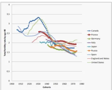
In the 20th century, growth theorists paid particular attention to interactions between, on the one hand, the production of goods, and, on the other hand, fertility behavior, that is, the production of men. When studying those inter-actions, they have mainly focused on one aspect of fertility: the number or quantum of births. From that perspective, the key stylized fact to be explained is the declining trend in fertility.1 That decline is illustrated on Figure 1, which shows the completed total fertility rate (TFR) for cohorts of women aged 40 in industrialized countries. That fertility decline was explained through various channels, such as the rise in the opportunity costs of children (Barro and Becker 1989), a shift from investment in quantity towards quality (education) caused by lower infant mortality (Erhlich and Lui 1991), a rise in women’s relative wages (Galor and Weil 1996), and the rise of contraception (Strulik 2016).
Figure 1: Completed cohort fertility by age 40 (source: Human Fertility Database)
Although those models cast substantial light on the interactions between fertility and development, their exclusive emphasis on the quantum of births leaves aside another important aspect of fertility, which has a strong impact on economic development: the timing or tempo of births. Studying the tempo of births - and not only the quantum of births - matters for understanding long-run economic development, because of two distinct reasons.
First, theoretical papers, such as Happel et al (1984), Cigno and Ermisch (1989) and Gustafsson (2001), studied, at the microeconomic level, the
mech-1Note that, although the long-run trend of the TFR is decreasing, the TFR can nonetheless
anisms by which the birth timing decision is related to education and labor supply decisions. A lower wage early in the career reduces the opportunity cost of an early birth, and pushes towards advancing births (substitution e¤ect), but limits also the purchasing power, which pushes towards postponing births (income e¤ect). Moreover, investing in education raises the purchasing power in the future (which pushes towards postponing births), but, at the same time, raises also the opportunity cost of future children (which pushes towards ad-vancing births). Those strong interactions between birth timing, education and labor decisions at the temporary equilibrium motivate the study, in a dynamic model, of how development a¤ects - and is a¤ected by - birth timing.
Second, there is also strong empirical evidence supporting the existence of complex, multiple interactions between the tempo of births and various eco-nomic variables, with causal relations going in both directions. Demographic studies show that the tempo of births is strongly correlated with the education level, which a¤ects the human capital accumulation process (see Smallwood, 2002, Lappegard and Ronsen 2005, Robert-Bobée et al 2006). Moreover, sev-eral works, such as Schultz (1985), Heckman and Walker (1990) and Tasiran (1995), show that a rise in women’s wages tends to favor a postponement of births.2 There is also evidence that the wage level is a¤ected by the timing of births (see Miller 1989, Joshi 1990, 1998, Dankmeyer 1996).
The timing of births has varied signi…cantly during the 20th century, as illustrated on Figure 2, which shows the cohort mean age at birth by age 40.3 Whereas the patterns di¤er across countries, Figure 2 reveals an important stylized fact: the average age at motherhood exhibits, across cohorts, a U-shaped pattern. The average age at motherhood has been …rst decreasing for cohorts born before 1940/1950, and, then, has been increasing for later cohorts.4 The U-shaped cohort mean age at birth raises several questions. A …rst question concerns the economic causes and consequences of that non-monotonic pattern. How can one explain that economic development is associated …rst with advancing births, and, then, with postponing births? How can one relate this stylized fact with income and substitution e¤ects, and with the education decision? Another key question concerns the relation between the dynamics of the quantum of births (Figure 1) and the tempo of births (Figure 2). Why is it the case that, at a time of strong fertility decline, cohorts tended to advance births, and, then, tended to postpone births once total fertility was stabilized? Exploring the relationship between the quantum and the tempo of births is most crucial for understanding long-run development, and, in particular, the conditions allowing for an economic take-o¤. Economic development is often associated with the decline of fertility, but, at the same time, as long as the age
2Those studies focused on Sweden. Similar results were shown for Japan (Ermish and
Ogawa 1994), for Canada (Merrigan and Saint-Pierre 1998), and for the UK (Joshi 2002).
3The cohort mean age at birth by age 40 is computed for all births combined (and not
only for …rst births). As such, it is likely to depend on the quantum of births (women having more children being likely to be older, on average, when giving birth to a child). This paper focuses precisely on this relation between the tempo of births and the quantum of births.
4Note that the timing of the reversal varies across countries. For instance, in Russia, the
at motherhood remains low, this may prevent investments in higher education, and, hence, prevent the emergence of a sustainable economic take-o¤. Therefore, in order to understand the emergence of the take-o¤, one must go beyond the study of the quantity of births, to examine also the timing of births.
The goal of this paper is precisely to cast some light on the relation between the quantum of births, the tempo of births, and economic development. For that purpose, we propose to adopt a uni…ed growth approach. As pioneered by Galor (see Galor and Moav, 2002, Galor, 2010), the uni…ed growth approach pays a particular attention to the relation between quantitative changes (i.e. changes in numbers) and qualitative changes (i.e. changes in the form of relations between variables). Qualitative changes are here studied by means of regime shifts, which are achieved as the economy develops, and which cause major changes in the relations between fundamental variables.5 As such, the uni…ed growth approach is most adequate to study the U-shaped pattern exhibited by the tempo of births.
Figure 2: Cohort mean age at birth by age 40 (Source: Human Fertility Database)
For that purpose, this paper develops a three-period overlapping generations (OLG) model with lifecycle fertility, that is, with two fertility periods (instead of one as usually assumed). Individuals can thus decide not only the quantum of births, but, also, how they allocate those births along their lifecycle, that is, the tempo of births. In order to study the interactions between birth timing and education, we also assume that individuals can choose how much they invest in their education when being young, which will a¤ect their future productivity (and, hence, the opportunity cost of late births).
5Recent works in that approach include de la Croix and Licandro (2013), de la Croix and
Anticipating our results, we show that, depending on the prevailing level of human capital, the temporary equilibrium takes three distinct forms, which corresponds to three distinct regimes. In the …rst regime, individuals do not invest in education, and rises in income push them towards advancing births. In the second regime, individuals start investing in education, but education remains so low that income rises still make individuals advance births. Then, once human capital is su¢ ciently high, the economy enters a third regime, where income growth favors postponing births.
Our dynamic lifecycle fertility model can thus rationalize both the decrease in fertility and the U-shaped pattern of the mean age at birth. That rationalization of the non-monotonic relation between development and birth timing is achieved by means of regime shifts as the economy develops, without having to rely on exogenous shocks. Besides this analytical …nding, we also explore the capacity of our model to replicate numerically the dynamics of the quantum and the tempo of births. Taking the case of Swedish women cohort born between 1876 and 1966, we show that our model can reasonably …t the patterns of the cohort total fertility rate and the cohort mean age at motherhood.
Our paper is related to several branches of the literature. First of all, it complements microeconomic studies of birth timing, such as Happel et al (1984), Cigno and Ermisch (1989) and Gustafsson (2001), which examine birth timing decisions in a static setting, whereas we propose to draw the corollaries of those decisions for long-run dynamics. Second, we also complement recent works focusing on the relation between birth timing and long-run development, such as, in continuous time, d’Albis et al (2010), and, in discrete time, Momota and Horii (2013), and Pestieau and Ponthiere (2014, 2015). Those papers examined the relation between, on the one hand, physical capital accumulation, and, on the other hand, the quantum and tempo of births. We complement those papers by paying attention to the interactions with the education decision and the human capital accumulation process. Moreover, another extra value of our paper lies in the fact that it adopts a uni…ed growth approach, where regime shifts are used to rationalize the non-monotonic pattern exhibited by the tempo of births.
The rest of the paper is organized as follows. The model is presented in Section 2. The temporary equilibrium is studied in Section 3, which character-izes the three possible regimes. Section 4 explores the long-run dynamics of our economy. Section 5 illustrates our …ndings numerically, by focusing on the case of Swedish women cohorts born between 1876 and 1966. Section 6 concludes.
2
The model
Let us consider a three-period OLG model with lifecycle fertility. Time goes from 0 to +1. Each period has a unitary length. Period 1 is childhood, during which the child is raised by the parents, and does not make any decision. Period 2 is early adulthood, during which individuals work, consume, have ntchildren and invest in higher education. Period 3 is mature adulthood, during which individuals work, consume, and can complete their fertility by having mt+1
children. Figure 3 shows the formal structure of the model.
Figure 3: The lifecycle fertility model.
Production Production involves labor and human capital. The output of an agent at time t, denoted by yt, is equal to:
yt= ht`t (1)
where htis the human capital of the agent at time t, while `tis the labor time. Human capital accumulation When becoming a young adult at time t, each agent is endowed with a human capital level ht> 0.6 This human capital level determines the marginal productivity of his labor when being a young adult.
The young adult can invest in higher education, in such a way as to in-crease his human capital stock at the next period. Human capital accumulates according to the law:
ht+1= (v + et) ht (2)
where et denotes the level of e¤ort/investment in higher education, while v is an accumulation parameter, which determines the rate at which human capital accumulates in the absence of higher education (i.e. when et= 0). We assume here, for analytical tractability, that education takes the form of a non-monetary, non-temporal, physical e¤ort, which can take any positive value.
6This is true for all individuals born in t 1, whaterver these are themselves early or late
children. This uniformity of endowments across children allows us to keep a representative agent structure, unlike in Pestieau and Ponthiere (2016), where early and late children, who di¤er in terms of time constraints, are studied as two distinct populations.
Throughout this paper, we will also suppose that v > 1, that is, that even in the absence of higher education, individuals can become more productive over time. Human skills can improve despite the absence of higher education, because either of a standard learning by doing mechanism, or of an exogenous technological progress raising the productivity of labor.
Budget constraints It is assumed that raising a child has a time cost q 2 ]0; 1[. That cost is supposed to be the same for early and late children. Thus, assuming that there is no savings, so that each agent consumes what he produces at each period of life, the budget constraint at early adulthood is:7
ct= ht(1 qnt) (3)
where ct denotes consumption at early adulthood for a young adult at time t. The budget constraint at mature adulthood is:
dt+1= ht+1(1 qmt+1) (4)
where dt+1 denotes consumption at mature adulthood for a mature adult at time t + 1.
Preferences Individuals derive some utility from consumption and from having children. They also derive disutility from investing e¤orts in higher education.
Individuals are endowed with preferences having a log linear form:
log (ct+ ) log (et+ ) + log(dt+1+ ") + log(nt) + log(mt+1) (5) where > 0, > 0, > 0, > 0, > 0, " > 0, > 0 and > 0 are preference parameters. and capture the weight assigned to consumption during the life. captures the disutility of higher education e¤orts. (resp. ) captures the taste for early (resp. late) fertility. Parameters , and " are used to allow for the emergence of various types of temporary equilibria, exhibiting either interior or corner solutions for the choice variables.
An important feature of the above utility function is that it exhibits limited substitutability between early births and late births. The main justi…cation for this feature is that, in the same way as there is no perfect substitutabil-ity for the allocation of consumption across time periods, there is no perfect substitutability for the allocation of births across time periods.
3
The temporary equilibrium
At the beginning of early adulthood, individuals choose the higher education e¤ort et, the number of early children nt, and the number of late children mt+1,
7It is assumed here that investing in higher education does not involve either monetary
costs or time costs. Higher education is here treated as a kind of e¤ort, which can raise future human capital, but at the cost of some disutility at early adulthood. See below on this.
in such a way as to maximize their lifetime welfare, subject to their budget constraints. The problem can be written as:
max et;nt;mt+1
log (ht(1 ntq) + ) log (et+ )
+ log((v + et)ht(1 mt+1q) + ") + log(nt) + log(mt+1) The …rst-order conditions (FOCs) for, respectively, optimal interior levels of education et, early fertility ntand late fertility mt+1, are:
(et+ ) = ht(1 mt+1q) (v + et)ht(1 mt+1q) + " (6) htq ht(1 ntq) + = nt (7) (v + et)htq (v + et)ht(1 mt+1q) + " = mt+1 (8)
The …rst FOC characterizes the optimal interior level of higher education e¤ort. It states that the optimal higher education e¤ort equalizes the marginal disutility of education e¤ort (LHS) and the marginal utility gain from extra consumption at mature adulthood thanks to education (RHS).
The second FOC, which characterizes the optimal early fertility level, equal-izes the marginal utility gain from early fertility (RHS) with the marginal utility loss from early fertility (LHS). Note that, since > 0, the marginal utility loss of early births depends on the prevailing level of human capital. This would not be the case under = 0, since in that case the income and substitution e¤ects would cancel each other, making fertility independent from human capital.
Finally, the third FOC characterizes the optimal late fertility level. It equal-izes the marginal utility gain from late births (RHS) with the marginal utility loss from late births (LHS). Note that, under " > 0, the latter depends on the education level, which a¤ects both the purchasing power at mature adulthood and the opportunity cost of late births.
Whereas the 3 FOCs characterize a temporary equilibrium with interior levels for education et, early fertility ntand late fertility mt+1, such an interior temporary equilibrium is not necessarily reached, depending on the level of human capital at time t. Proposition 1 summarizes the three di¤erent regimes. Those regimes di¤er not only in terms of the levels of education et and total fertility (nt+ mt+1), but, also, in terms of the timing of births, which is here measured by the ratio early births / late births, Rt mnt+1t .
Proposition 1 De…ne the function: e(ht)
[ht +']+p2 (ht)
2ht! , where (ht)
[ht + ']2+ 4ht!v ( v ) ht h , and where 2 v (v + ) , '
" ( + ), ! ( ) and h v("( v+ v)).
De…ne ~h as the solution to: e(h) + (h + ) e0(h) = "(v + e(h))2 v.
There exist sets of values for the parameters such that the level of human capital de…nes three regimes:
Regime I: if ht< h, then: eIt = 0 nIt = (ht+ ) htq ( + ) > 0 mIt+1 = (vht+ ") vhtq ( + )> 0 RIt = (ht+ ) v ( + ) ( + ) (vht+ ") > 0 @eI t @ht = 0; @nI t @ht < 0; @mIt+1 @ht < 0; @RI t @ht > 0 Regime II: if h < ht< ~h, then:
eIIt = e(ht) > eIt nIIt = (ht+ ) htq ( + ) < nIt mIIt+1 = ((v + e(ht))ht+ ") (v + e(ht))htq ( + ) < m I t+1 RIIt = (ht+ ) (v + e(ht)) ( + ) ( + ) ((v + e(ht))ht+ ") > R I t @eII t @ht > 0;@n II t @ht < 0;@m II t+1 @ht < 0;@R II t @ht > 0
Regime III: if ~h < ht, then: eIIIt = e(ht) > eIIt nIIIt = (ht+ ) htq ( + ) < n II t mIIIt+1 = ((v + e(ht))ht+ ") (v + e(ht))htq ( + ) < mIIt+1 RIIIt = (ht+ ) (v + e(ht)) ( + ) ( + ) ((v + e(ht))ht+ ") < R II t @eIII t @ht > 0; @nIII t @ht < 0; @mIII t+1 @ht < 0; @RIII t @ht < 0 Proof. See the Appendix.
Proposition 1 states that, depending on the prevailing level of the human capital stock, there can exist, in our economy, three distinct regimes.
Under the …rst regime, human capital is low, and there is no higher educa-tion. The reason is that the marginal return of investing in education is, given the low human capital stock, too low with respect to its marginal disutility,
which makes investment in higher education not worthy. Quite interestingly, in that regime, a rise in human capital reduces both early and late fertility, but pushes parents towards having a larger proportion of early births (i.e. human capital raises the ratio Rt, that is, the ratio early births over late births). Thus, in Regime I, the rise in income pushes towards advancing births. The intuition behind that result is that, under the assumption " > v, we have that, under a zero education, the marginal utility loss from foregone consumption due to early births is, ceteris paribus, less increasing with htthan the marginal utility loss from foregone consumption due to late births.8
In the second regime, higher education is now strictly positive, since the human capital is su¢ ciently large, so that the marginal return from investing in education is su¢ ciently high so as to counterbalance the marginal disutility of investing in education. In that second regime, education is increasing in human capital. Note also that, in Regime II, fertility at both periods is now lower than under Regime I. But the accumulation of human capital - and, hence, the rise in income - has still the consequence of advancing births.
In the third regime, fertility is even lower than in the two previous regimes, but there is an important qualitative change. Whereas the rise in income used to push towards advancing births in Regimes I and II, this is no longer the case in Regime III, where the rise in income pushes towards postponing births (that is, human capital reduces the ratio Rt). This third regime coincides with what could be called the modern regime, where the decline in fertility is associated with births postponement. Note that, whereas Regime III may seem, at …rst glance, quite similar to Regime II, these di¤er signi…cantly on quantitative and qualitative aspects. From a quantitative perspective, Regime III is characterized by lower fertility, and by a higher average age at motherhood. From a qualitative perspective, Regime III is characterized by an inversion, with respect to Regime II, of the relation between income growth and birth timing.
In sum, Proposition 1 shows that, depending on the prevailing level of human capital, the economy can be characterized by three distinct regimes, where the relations between income, the quantum at birth and the tempo of births vary. Each of those regimes can be regarded as a particular stage of development. The next section aims at describing how the economy shifts from one regime to the next as human capital accumulates.
4
Long-run development
In order to study how our economy evolves over time, this section will …rst consider the dynamics of human capital accumulation. In a second stage, we will study the dynamics of the quantity and the timing of births.
8To better see this, note that, if were equal to 0, the marginal utility loss from foregone
4.1
Human capital growth
Starting from an initial human capital level h0 < h, the economy is initially in Regime I. Under that regime, education investment is equal to zero and human capital grows at an exogenous, positive rate v. Once the human capital stock crosses the threshold h, the economy enters Regime II, under which education e¤ort becomes positive. Hence the growth rate is now:
gt+1II = v + eIIt > gIt+1= v
Once the human capital stock reaches a second threshold, equal to ~h > h, the economy enters into Regime III, where the human capital stock grows at a rate:
gIIIt+1 ht+1 ht
= v + eIIIt
Given that education e¤ort is increasing with human capital (so that eIII t > eII
t ), we obtain, when comparing the growth rates of human capital, that: gIIIt+1> gIIt+1> gt+1I = v
Thus, once it has reached the modern regime (i.e. Regime III), the human capital stock grows even more quickly than under the two preceding regimes.
Note that, whereas human capital grows without limit in Regime III, we know, since education converges towards a …nite positive level (see Proof of Proposition 1 in the Appendix), that the growth rate of human capital converges asymptotically towards a positive level, equal to:
g1= v + lim h!1e(ht) = v + 2! + 2 r 2 2+ 8!v ( v ) 8!2 > 0
The following proposition summarizes our results.
Proposition 2 Under Regime I, the human capital stock grows at an
exogenous constant rate v > 0.
Under Regime II and Regime III, the human capital stock grows at a rate that is higher than v. That growth rate is increasing in education, which is itself increasing in ht:
gt+1III > gIIt+1> gt+1I = v
The growth rate of human capital tends, in the long-run, towards the level: g1= v + 2! + 2 r 2 2+ 8!v ( v ) 8!2
Proof. See above.
Our model thus predicts an acceleration of human capital accumulation as the economy develops. The …rst stage of development (i.e. Regime I) is charac-terized by lower human capital accumulation, since education e¤orts are limited at that stage. But when the economy enters Regime II, education e¤orts be-come positive, and growing with the stock of human capital, which makes the growth of human capital stock even stronger than in Regime II. Finally, once the economy reaches the second threshold, and enters Regime III, the growth rate of human capital is even larger than in Regime II. The reason is that, in Regime III, human capital accumulation pushes towards births postponement, which has here the impact of increasing even more the attractiveness of higher education investment, which in turn strengthens human capital accumulation.
4.2
Quantum and tempo of births
Besides the dynamics of human capital accumulation, one may also be interested in studying the evolution of total fertility and of the timing of births when the economy develops. For that purpose, we can, in our model, de…ne the cohort total fertility rate (TFR) as:
T F Rt nt+ mt+1
as well as the cohort mean age at birth (MAB) as:
M ABt nt 1 + mt+1 2
nt+ mt+1
where it is here assumed that individuals having children during a period have those children at the beginning of the period (and thus have age 1 for early births and age 2 for late births).
Again, we can consider, as a starting point, an economy with initial human capital h0< h. In Regime I, human capital accumulates at a rate v. Given that both nt and mt+1 are decreasing in human capital under either Regimes I, II or III, it is straightforward to deduce that the cohort TFR is decreasing as the economy develops:
T F RIt > T F RIIt > T F RIIIt
Concerning the evolution of the cohort mean age at birth, one can notice that the MAB can be rewritten as:
M ABt= Rt+ 2 Rt+ 1
The mean age at birth is thus decreasing in the ratio Rt. From Proposition 1, we know that the ratio Rt is, in Regimes I and II, increasing with human capital accumulation, so that we have:
However, once the economy has entered Regime III, the relation between human capital accumulation and birth timing is inverted, and the ratio Rt becomes decreasing with human capital, so that we know have:
M ABIIt < M ABtIII
Thus, as the economy develops, we can observe a monotonic decline in the quantum of births (TFR), and a non monotonic, U-shaped relation in the MAB. Note also that, since education converges asymptotically towards a positive constant, it is also the case that both early and late fertility converges towards a constant in the long-run. These are equal to, respectively:
lim ht!1 nt = q ( + )> 0 lim ht!1 mt+1 = q ( + )> 0
As a consequence, the TFR and MAB converge asymptotically towards, respectively:
T F R1 =
q ( + )+q ( + )
M AB1 = ( + ) + 2 ( + )
( + ) + ( + ) The following proposition summarizes our results.
Proposition 3 Comparing the levels of the cohort TFR across regimes, we have a monotonic decline in TFR as the economy develops, and goes from Regime I to Regimes II and III:
T F RIt > T F RtII > T F RIIIt
Comparing the levels of the cohort MAB across regimes, we have a non monotonic, U-shaped pattern for the MAB as the economy develops, and goes from Regime I to Regimes II and III:
M ABtI > M ABtII < M ABtIII
The cohort TFR and the cohort MAB converge asymptotically towards, respectively:
T F R1 =
q ( + )+q ( + )
M AB1 = ( + ) + 2 ( + )
Proof. See above.
In the light of Proposition 3, it is possible to rationalize the observed evolu-tion of the quantum and the tempo of births as the economy develops. While the …rst stages of development are characterized by large quantity of children and high age at motherhood (i.e. high TFR and high MAB), the quantum of births decreases as the economy develops, whereas the timing of births follows a non-monotonic pattern: economic development …rst pushes towards advancing births (i.e. a lower MAB), and, then, towards postponing these (i.e. a higher MAB).
5
Numerical analysis
The previous Sections show that our model can, qualitatively, explain or ratio-nalize the global patterns exhibited by the quantum and the tempo of births. One may want to go further in the replications, and wonder to what extent it is possible, by calibrating our model, to reproduce the TFR and MAB patterns for a real-world economy. This is the task of this Section.
For that purpose, we will consider here the case of Sweden, for which we have the longest time series of cohort TFR and cohort MAB in the Human Fertility Database. Figure 4 shows the patterns of the TFR at age 40 for cohorts born between 1876 and 1974, while Figure 5 shows the pattern of the MAB at age 40 for the same cohorts. As shown on Figure 4, there has been a substantial decline in the quantum of births across the periods considered, from about 3.2 children per women for the cohort born in 1876 towards less than 2 children per women for the cohort born in 1974. Note, however, that there has been some short-run ‡uctuations in the TFR, with some rebound for cohorts born in the 1900s, as well as a second rebound for those born in the 1930s. Concerning the evolution of the MAB (Figure 5), the curve exhibits a U-shaped pattern, as mentioned in Section 1. The MAB was quite high - around age 30 - for Swedish women born in 1876, but then strongly declined, to reach about 26 years for cohorts born in the 1940s. Then, there was a substantial births postponement for cohorts born after 1950. For cohorts born in the 1970s, the MAB is close to its level for cohorts born one century before. Note, however, that the MAB has also exhibited short-run ‡uctuations. In particular, cohorts born in the 1910s have exhibited a higher MAB than those born in the 1900s.
Figure 4: Cohort TFR at age 40 for Swedish cohorts 1876-1974 (source: Human Fertility
Database).
Figure 5: Cohort MAB by age 40 for Swedish cohorts 1876-1974 (Source: Human Fertility
Database).
Figure 5 makes appear a major di¢ culty in trying to replicate quantitatively the observed pattern of the tempo of births by means of a discrete time OLG model with relatively long fertility periods (and thus with few coexisting
co-horts). The di¢ culty lies in the fact that the timing of births has exhibited massive and quick changes in a very small number of (annual) cohorts. Clearly, for cohorts born in the …rst part of the 20th century, the MAB has decreased by about 3 years (about 10 %) in just 25 (annual) cohorts. Moreover, for co-horts born in the second part of the 20th century, a very quick and massive postponement of births, with a 4-year rise in just 25 (annual) cohorts. When transposed to our 3-period OLG model, those changes imply strong variations in MAB over just a few cohorts. An even larger challenge comes from the fact that, for cohorts born in the 20th century, the TFR has remained relatively stable. One must thus …nd a way to reconcile strong changes in the tempo of births with low changes in the quantum of births.
Given that, in our model, periods are of about 18 years (which implies having early children at age 18 and late children at age 36), we will focus here on the TFR and MAB for cohorts born in years 1876, 1894, 1912, 1930, 1948 and 1966. Figures 6 and 7 below show the actual levels of TFR and MAB for those cohorts (in continuous traits), as well as the levels of those variables that are simulated under some particular vector of values for the structural parameters of our economy (in discontinuous traits).9 Note that, unlike in the theoretical model, we have here assumed cohort-speci…c time cost of children qt, in such a way as to be able to perfectly …t the cohort TFR pattern (Figure 6).10 Given that our main focus is on the timing of births rather than on the quantum, and given that the tempo of births is invariant to the parameter q, this does not constitute a strong restriction for the purpose at hand.
Figure 6: Cohort TFR: data and model.
9Figures 6 and 7 rely on the following values for parameters. h
0 = 0:001, v = 3:50,
= 0:55, = 0:61, = 0:0065, = 0:0035, " = 0:02, = 10:55, = 0:0075, = 0:66.
1 0Figure 6 relies on period-speci…c cost of children: q
0 = 0:725, q1 = 0:322, q2 = 0:125,
Figure 7: Cohort MAB: data and model
As shown on Figure 7, our model is able to replicate, over the Swedish cohorts considered, the non-monotonic, U-shaped pattern of cohort mean age at birth. Clearly, the model can replicate that, as the economy develops, there is …rst a process of advancing births, and, then, of postponing births.
The replication of this non-monotonic MAB pattern without using any ex-ogenous shock is achieved by means of the multiplicity of regimes in our model. The economy starts in Regime I (no higher education) for cohorts born in 1876, 1894 and 1912. In that regime, the rise in incomes generates an advancement of births, that is, a fall of the MAB. Then, the economy enters Regime II (positive higher education) for women born in cohort 1930. During that regime, there is also an advancement of births. The economy enters Regime III for cohorts born after 1948, for which the rise in income will be associated not with an advancement, but with a postponement of births.
In the light of this, it appears that our uni…ed growth model can rationalize the dynamics of the tempo of births as a succession of regime shifts. Besides those strengths, it is also worth noticing some limitations of our numerical analy-sis. First, our model can only replicate the overall trend of the MAB, without being able to replicate short-term ‡uctuations in the MAB, such as the (tran-sitory) postponement of births for cohorts born in the 1900s. However, given that our analysis focuses on long-run trends, this limitation is not problematic. A more important comment on Figure 7 concerns the fact that, although the model can replicate the U-shaped pattern of the MAB, it exhibits nonetheless, from a quantitative perspective, some limitations in being able to reproduce the very strong growth in the MAB just after the reversal. The model captures the non-monotonicity of the MAB pattern, but can hardly reproduce such a strong reversal in a few cohorts. This suggests that other factors - not present in our model - may have also a¤ected the magnitude of the recent births postponement.
6
Conclusions
In the recent decades, economists have paid a substantial attention to the expla-nation or rationalization of the dynamics of the quantum of births, in relation with economic development. Those analyses were most successful in provid-ing explanations for the long-run declinprovid-ing trend in fertility, such as the rise of the opportunity cost of children, a change in the direction of intergenerational transfers, or the fall of infant mortality. However, most analyses were made in models with a unique fertility period. As such, those analyses could bring little light on the dynamics of the tempo of births, and on its relationship with economic development.
The goal of this paper was precisely to study the relationship between eco-nomic development, the quantum of births and the tempo of births. Our purpose was to build a dynamic model of lifecycle fertility that can rationalize the ob-served patterns of the quantum and the tempo of births. In particular, our goal was to build a model that can explain that, as the economy develops, the mean age at birth tends …rst to decline, and, then, tends to grow.
For that purpose, we developed a 3-period OLG model with lifecycle fertility (i.e. 2 fertility periods), where individuals choose not only their education and the total number of children, but, also, how they allocate births along their lifecycle. Following the increasingly large uni…ed growth literature, we consid-ered preferences that are su¢ ciently general so as to allow for multiple types of temporary equilibria, leading to di¤erent regimes.
When studying that model, we showed that, depending on the prevailing level of human capital, an economy could be in three distinct regimes. In Regime I, there is no education, and fertility is high. In that traditional regime, a rise in income pushes towards advancing births, since this raises relatively more the opportunity cost of late births in comparison to early births. Then, once human capital reaches some threshold, individuals start investing in education. In that second regime, fertility is lower, but it is still the case that, as income grows, births are being advanced. However, once the human capital stock is su¢ ciently large so as to reach a second threshold, the relationship between income growth and births postponement is reversed, and higher incomes lead now to postponing births (unlike in Regimes I and II).
The identi…cation of three distinct regimes casts signi…cant light on the rela-tion between economic development and fertility behaviors (quantum and tempo of births). First of all, our model can explain why advanced industrialized economies exhibit, since the 1970s, both low fertility and births postponement. This coincides with Regime III examined in our model. But our framework can also cast some light on the situation of other, less advanced countries. Some developing countries, for instance in Africa, exhibit declining fertility trends, but still face strong economic di¢ culties, which prevent the economic take-o¤. Our model provides an explanation for this situation: those countries remain in Regime II, where births still arise quite early in life, which prevents large investment in education, and, hence, limits the possibility of an economic take-o¤. Thus, from the perspective of understanding the emergence of an economic
take-o¤, focusing only on the quantity of births does not su¢ ce, since the timing of births matters as much as the quantity of births.
Finally, in order to have a more precise idea of the extent to which our model can …t the data, we also illustrated our model numerically, by focusing on the case of Swedish cohorts born between 1876 and 1966. We showed that our model can approximately replicate the observed U-shaped pattern of the mean age at birth. Our model provides a simple way to rationalize the substantial changes in birth timing that were observed during the 20th century. Although our numerical simulations illustrate the explanatory potential of our model, it remains true that the model can only replicate long-run trends, and not short-run ‡uctuations. Moreover, the model cannot fully replicate the magnitude of the rise in MAB observed for cohorts born after 1960. This suggests that other factors may have been at work in the postponement of births. Hence, much work remains to be done to develop a more general model of lifecycle fertility.
7
References
Barro, R., Becker, G. (1989). Fertility choices in a model of economic growth. Econo-metrica, 57, 481-501.
Cigno, A., Ermisch, J. A microeconomic analysis of the timing of births. European Eco-nomic Review, 33, 737-760.
Dankmeyer, B. (1996). Long-run opportunity-costs of children according to education of the mother in the Netherlands, Journal of Population Economics, 9, 349-361.
D’Albis, H., Augeraud-Veron, E., Schubert, K. (2010): Demographic-economic equilibria when the age at motherhood is endogenous. Journal of Mathematical Economics, 46(6), 1211-1221.
De la Croix, D., Licandro, O. (2013). The child is the father of man: implications for the demographic transition, Economic Journal, 123, 236-261.
De la Croix, D., Mariani, F. (2015). From polygyny to serial monogamy: a uni…ed theory of marriage institutions. Review of Economic Studies, 82, 565-607.
Ehrlich, I., Lui, F. (1991). Intergenerational trade, longevity and economic growth. Jour-nal of Political Economy, 99, 1029-1059.
Ermish, J., Ogawa, N. (1994). Age at motherhood in Japan, Journal of Population Economics, 7, 393-420.
Galor, O. (2010). The 2008 Lawrence R. Klein Lecture-Comparative Economic Develop-ment: Insights From Uni…ed Growth Theory. International Economic Review, 51, 1-44.
Galor, O., Moav, O. (2002). Natural Selection and the Origin of Economic Growth. Quarterly Journal of Economics, 117(4), 1133-1191.
Galor, O., Weil, D. (1996). The gender gap, fertility and growth. American Economic Review, 86, 374-387.
Gustafsson, S. (2001). Theoretical and empirical considerations on postponement of ma-ternity in Europe. Journal of Population Economics, 14, 225-247.
Happel, S., Hill, J., Low, S. (1984). An economic analysis of the timing of child-birth. Population Studies, 38, 299-311.
Heckman, J., Walker, J. (1990). The relationship between wages and income and the timing and spacing of births : evidence from Swedish longitudinal data, Econometrica, 58, 1411-1441.
Human Fertility Database. Max Planck Institute for Demographic Research (Germany) and Vienna Institute of Demography (Austria). Available at www.humanfertility.org (data downloaded on October 2016).
Joshi, H. (1990). The cash alternative costs of childbearing: an approach to estimation using British data, Population Studies, 44, 41-60.
Joshi, H. (1998). The opportunity costs of childbearing: more than mother’s business. Journal of Population Economics, 11, 161-183.
Joshi, H. (2002). Production, reproduction, and education: women, children and work in a British perspective, Population and Development Review, 28, 445-474.
Lappegard, T., Ronsen, M. (2005). The multifaceted impact of education on entry into motherhood. European Journal of Population, 21, 31-49.
Lindner, I., Strulik, H. (2015). From Tradition to Modernity: Economic Growth in a Small World. Journal of Development Economics, 109, 17-29.
Merrigan, P., Saint-Pierre, Y. (1998). An econometric and neoclassical analysis of the timing and spacing of births in Canada from 1950 to 1990, Journal of Population Economics, 11, 29-51.
Miller, A. (2009). Motherhood delay and the human capital of the next generation. American Economic Review, 99, 154-158.
Momota, A., Horii, R. (2013). Timing of childbirth, capital accumulation, and economic welfare. Oxford Economic Papers, 65(2), 494-522.
Pestieau, P., Ponthiere, G. (2014). Optimal fertility along the life cycle. Economic Theory, 55(1), 185-224.
Pestieau, P., Ponthiere, G. (2015). Optimal life-cycle fertility in a Barro-Becker economy. Journal of Population Economics, 28 (1), 45-87.
Pestieau, P., Ponthiere, G. (2016). Long term care and birth timing. Journal of Health Economics, 50, 340-357.
Robert-Bobée, I., Rendall, M., Couet, C., Lappegard, T., Ronsen, M., Smallwood, S. (2006). Âge au premier enfant et niveau d’études: une analyse comparée entre la France, la Grande-Bretagne et la Norvège, Données sociales – La société française, 69-76
Schulz, T. (1985). Changing world prices, women’s wages and the fertility transition: Sweden 1860-1910. Journal of Political Economy, 93, 1126-1154.
Smallwood, S. (2002). New estimates of trends of births by birth order in England and Wales, Population Trends, 108, p. 32-48.
Strulik, H. (2016). Contraception and development: a uni…ed growth theory. Interna-tional Economic Review, forthcoming.
Tasiran, A. (1995). Fertility Dynamics: Spacing and Timing of Births in Sweden and the United States, Amsterdam, Elsevier, 1995.
8
Appendix
8.1
Proof of Proposition 1
In this Appendix, we show that, when the structural parameters satisfy the conditions: " > v, > v, > , < 0, ' > h , " 2 2+4!v( v ) 4!2 > v + 2! 1 "v + 2 q 2 +4!v( v ) 4!2 1 2" v + 2! , 2h! v ( v ) h > ' h + ' , ( (~h)) 1=2 0 (~h) 2~h + 2 p (~h) ' (~h)3 < ( (~h)) 3=2 [ 0(~h)]2 8 1 + ~h ,
then the human capital level de…nes the three regimes described in Proposi-tion 1.
Existence of a threshold for Regime II From the FOC for early fer-tility, we have:
nt=
[ht+ ] htq( + )
> 0 From the FOC for late fertility, we have:
mt+1=
[(v + et)ht+ "] (v + et)htq [ + ] > 0 From the FOC for education,
(et+ ) = ht(1 mt+1q) (v + et)ht(1 mt+1q) + " we obtain: et= ht(1 mt+1q) " vht(1 mt+1q) (1 mt+1q) ( ht ht)
Note that education equals zero when:
ht(1 mt+1q) < " + vht(1 mt+1q) Substituting for mt+1when et= 0, that expression becomes:
ht 1 [vht+ "] vhtq [ + ]q < " + vht 1 [vht+ "] vhtq [ + ]q ht vht[ + ] [vht+ "] vht[ + ] ( v) < " ht < "v [ + ] + " ( v) v ( v) ht < " ( v + ) v ( v)= h
Hence, when ht < h, we have eI t = 0 and nIt = [ht+ ] htq( + ) > 0 and m I t+1 = [vht+"]
vhtq[ + ] > 0: This situation coincides with Regime I.
Note that, in that regime, we obviously have a corner solution for education, so that @et @ht = 0. We also have @nt @ht = q( + ) [ht]2 < 0 @mt+1 @ht = " vq [ + ] [ht]2 < 0
Note that the ratio of early births over late births, Rt=
[ht+ ] htq( + ) [vht+"] vhtq[ + ] = [ht+ ]v[ + ] ( + ) [vht+"],
varies with human capital as follows: @Rt @ht = v [ + ] ( + ) [vht+ "] [ht+ ] v [ + ] ( + ) v [( + ) [vht+ "]]2 = v [ + ] " v ( + ) [[vht+ "]]2 > 0
Given the assumption " > v , we have that, as human capital accumulates, births are being advanced.
Despite the absence of education, human capital grows at a rate v. When ht > h, it is no longer the case that education equals zero. Indeed, education equals zero when:
> ht(1 [vht+"] vhtq[ + ]q) vht(1 [vht+"] vhtq[ + ]q) + " () ht< " ( v + ) v ( v) = h
Thus when ht> h, that strict inequality cannot hold any more. It can be shown that, when ht> h, we necessarily have an interior education level et> 0. To see this, let us …rst write down the FOC for et:
(et+ )
= ht(1 mt+1q)
(v + et)ht(1 mt+1q) + "
Substituting for mt+1= (v+e[(v+et)htt)hq[ + ]t+"] in that FOC, we obtain:
(v + et)ht " + " ( + ) ( + ) ) = (v + et)ht " (v + et) ( + ) (et+ ) Hence e2t[ht ht ] +et[2vht " + " ( + ) (v + )ht + "] v ht + " + v2ht v " + v " ( + ) = 0
Hence e2tht[ ] + et[ht(2v (v + ) ) + " ( + )] vht( v ) + " ( + v ) = 0 Hence we have (ht) = [ht(2v (v + ) ) + " ( + )]2 4ht[ ] [ vht( v ) + " ( + v )]
The …rst term is positive. Given that the threshold is v("( v+ v)) > ht, we have herev("( v+ v)) < ht, which implies that [ vht( v ) + " ( + v )] < 0. Hence, provided > 0, we have (ht) > 0:
Note that, given h = v("( v+ v)), we can rewrite the above expression as: (ht) = [ht(2v (v + ) ) + " ( + )]2+ 4ht[ ] v ( v ) ht h
Using the notations 2v (v + ) , ' " ( + ) and ! ( ), we
have: (ht) = [ht + ']2+ 4ht! v ( v ) ht h with 0(h t) = 2 [ht + '] + 4! v ( v ) ht h + 4ht! [v ( v )] = 2 [ht + '] + 8ht! [v ( v )] 4! v ( v ) h
We can rewrite education as:
eIIt = [ht + '] +
2
p (ht) 2ht!
Notice that, when ht> h, we have (ht) > 0 andp2
(ht) > [ht + '], so that education is necessarily positive. Hence we have eIIt > 0 = eIt.
We have also, in that second regime,
nIIt = [ht+ ] htq( + ) mIIt+1 = (v + [ht +']+p2 (ht) 2ht! )ht+ " (v + [ht +']+p2 (ht) 2ht! )htq [ + ] = h 2vht! [ht + '] +p2 (ht) + 2!" i q [ + ] (2ht!v [ht + '] +p2 (ht))
Given that ht is higher in Regime II than in Regime I, we obviously have nIIt < nIt.
Regarding mIIt+1, we have: @mII t+1 @ht = h 2v! +12[ (ht)] 1=2 0(ht) i q [ + ] (2ht!v [ht + '] + 2 p (ht)) h 2vht! [ht + '] +p2 (ht) + 2!" i q [ + ] (2!v +12[ (ht)] 1=2 0(ht)) h q [ + ] (2ht!v [ht + '] + 2 p (ht)) i2 = [2!"] (2!v + 1 2[ (ht)] 1=2 0 (ht)) q [ + ] h (2ht!v [ht + '] +p2 (ht)) i2 < 0
Regarding the impact of human capital on the ratio Rt, we now have:
Rt= [ht+ ] htq( + ) [(v+e(h))ht+"] (v+e(h))htq[ + ] = [ht+ ] (v + e(ht)) [ + ] ( + ) [(v + e(ht))ht+ "] where e (ht) [ht +']+p2 (ht) 2ht! . We have: @Rt @ht = [ (v + e(ht)) ( + ) + (ht+ ) (e0(ht)) ( + )] ( + ) ((v + e(ht))ht+ ") [ (ht+ ) (v + e(ht)) ( + )] [( + ) (e0(ht)ht+ v + e(ht))] [( + ) ((v + e(ht))ht+ ")]2 = ( + ) ( + ) [(v + e(ht)) + (ht+ ) (e0(ht))] ((v + e(ht))ht+ ") [(ht+ ) (v + e(ht))] [ (e0(ht)ht+ v + e(ht))] [( + ) ((v + e(ht))ht+ ")]2 = ( + ) " [v + e(ht) + (ht+ ) e0(ht)] (v + e(ht)) 2 ( + ) [(v + e(ht))ht+ "]2 We have thus: @Rt @ht > 0 () ( + ) " [v + e(ht) + (ht+ ) e0(ht)] (v + e(ht))2 ( + ) [(v + e(ht))ht+ "]2 > 0 This implies: " [v + e(ht) + (ht+ ) e0(ht)] (v + e(ht))2 > 0 " [v + e(ht) + (ht+ ) e0(ht)] > (v + e(ht))2 " [v + e(ht) + (ht+ ) e0(ht)] > (v + e(ht))2
When education equals 0 (Regime I), that corner solution is insensitive to ht, and we have thus that the condition vanishes to " > v, which is necessarily satis…ed given our assumption on structural parameters. Thus, when ht< h, it is necessarily the case that @Rt
Regarding the impact of human capital on education, note that: e(ht) = [ht + '] +p2 (ht) 2ht! We have thus: e0(ht) = h +1 2[ (ht)] 1=2 0 (ht) i ht h [ht + '] + 2 p (ht) i 2! (ht)2 = 1 2[ (ht)] 1=2 0 (ht)ht 2 p (ht) + ' 2! (ht)2 = 2 p (ht) 2 0(h t)ht (ht) 2 p (ht) + ' 2! (ht)2 = 2 p (ht) 12 0(ht)ht (ht) 1 + ' 2! (ht)2 It is easy to show that 0(ht)ht
(ht) > 2, so that e 0(h t) > 0. Note that, 0(h t)ht (ht) = ht 2 [ht + '] + 4! v ( v ) ht h + 4ht! [v ( v )] [ht + ']2+ 4ht! v ( v ) ht h = 2 h 2 t 2+ 'ht + 4ht! v ( v ) ht h + 4h2t! [v ( v )] [ht + ']2+ 4ht! v ( v ) ht h Hence, 0(ht)ht (ht) > 2 implies: 2 h2t 2+ 'ht + 4ht! v ( v ) ht h + 4h2t! [v ( v )] > 2 [ht + ']2+ 8ht! v ( v ) ht h Or, alternatively: 0 > 2' (ht + ') 4ht! v ( v ) h
Note that the RHS is decreasing in ht, since < 0. Hence a su¢ cient condition for this inequality to hold for any ht h is thus:
0 > 2' h + ' 4h! v ( v ) h
Under this condition, education is growing in human capital for all ht h. Existence of a threshold for Regime III In the remaining of this proof, we show that there exists one level of human capital ~h > h that is such that, at ~
h, we have @Rt
@ht = 0 and that, for any ht> ~h, we have
@Rt
~
h de…nes the entrance of the economy in Regime III, where the relation between birth timing and human capital accumulation is reversed.
In order to prove the existence and uniqueness of that threshold ~h > h, let us …rst rewrite the condition for @Rt
@ht > 0 as:
e(ht) + (ht+ ) e0(ht) >
"(v + e(ht))
2 v
When httends to 0, the LHS tends to 0 and RHS tends to v "v 1 < 0 since " > v: Thus the condition is trivially satis…ed, and thus @Rt
@ht > 0.
When httends to h, we have:
LHS = 0 + h + e0(h) Note that e(ht) = [ht + '] + 2 p (ht) 2ht! Hence, at ht= h, we have: e0 h = ' 2! h 2 + 1 2 (h) 1=2 0 (h)h p2 (h) 2! h 2 = ' 2! h 2 + 1 2 h h + ' 2i 1=2 0(h)h q2 h + ' 2 2! h 2 = ' 2! h 2 + 0(h)h 2 h + ' 2 4! h 2 h + ' We have 0(h) = 2 [h t + '] + 4!v ( v ) 2ht h = 2 h + ' + 4!v ( v ) h Hence e0 h = ' 2! h 2 + 2 h + ' + 4!v ( v ) h h 2 h + ' 2 4! h 2 h + ' = ' 2! h 2 + hh + 'h + 2!v ( v ) hh h h 2+ 2h ' + '2i 2! h 2 h + ' = ' 2! h 2 + 'h + 2!v ( v ) hh '2 2! h 2 h + ' = v ( v ) h + ' > 0 which is positive, since ' > h .
Hence the LHS is: LHS = 0 + h + v ( v ) h + ' > 0 The RHS is, at ht= h: RHS = "(v + e(h)) 2 v = "(v + 0) 2 v = v "v 1 < 0
Thus, at h = h, it is also the case that the LHS exceeds the RHS, implying @Rt
@ht > 0.
Let us now examine how the LHS and the RHS of the expression: e(ht) + (ht+ ) e0(ht) =
"(v + e(ht))
2 v
vary when ht! +1. Clearly, given that the LHS exceeds the RHS for h h, a su¢ cient condition for the existence of a threshold ~h at which @Rt
@ht = 0 (that
is, at which the LHS and the RHS are equal) is that the RHS exceeds the LHS when ht ! +1. Then, by continuity, we would be able to conclude that the LHS and RHS intersect for some value of ht, which is precisely the threshold ~h
We have: lim ht!1 LHS = lim ht!1 [e(ht) + (ht+ ) e0(ht)] Let us decompose this in two components:
lim ht!1 LHS = lim ht!1 e(ht) + lim ht!1 (ht+ ) e0(ht)
Regarding the …rst component, we have, using the Hospital Rule: lim ht!1 e(ht) = lim ht!1 [ht + '] + 2 p (ht) 2ht! = 2! 0 + limht!1 2 p (ht) 2ht! = 2! 0 + limht!1 2 q [ht + ']2+ 4ht! v ( v ) ht h 2ht! = 2! 0 + limht!1 2 s [ht + ']2+ 4ht! v ( v ) ht h 4h2 t!2 = 2! 0 + 2 s lim ht!1 [ht + ']2+ 4ht! v ( v ) ht h 4h2 t!2 = 2! 0 + 2 s lim ht!1 2 [ht + '] + 4! v ( v ) 2ht h 8ht!2 = 2! 0 + 2 s lim ht!1 2 + 4! [v ( v ) 2] 8!2 = 2! + 2 r 2 2+ 8!v ( v ) 8!2 > 0
Regarding the second component, it is straightforward to show that it is equal to: lim ht!1 (ht+ ) e0(ht) = 0 since lim ht!1 e0(ht) = 0 Indeed, since e(ht) =
[ht +']+p2 (ht) 2ht! , we have: e0(ht) = ' 2!h2 t + 1 2[ (ht)] 1=2 0 (ht)ht p2 (ht) 2h2 t! e0(ht) = 1 2!h2 t ' +1 2 2 p (ht) 0(h t)ht (ht) 1 Hence lim ht!1 e0(ht) = 0 ' + lim ht!1 1 2 2 p (ht) 0(h t)ht (ht) 1 = 0 We thus have: lim ht!1 LHS = 2! + 2 r 2 2+ 8!v ( v ) 8!2
Concerning the RHS, we have: lim ht!1 RHS = lim h!1"(v + e(ht)) 2 v Given that: lim ht!1 e(ht) = 2! + 2 r 2 2+ 8!v ( v ) 8!2 we have: lim ht!1 RHS = " v + 2! + 2 r 2 2+ 8!v ( v ) 8!2 !2 v
Hence a su¢ cient condition for the RHS to be above the LHS when ht! 1 is: " v + 2! + 2 r 2 2+ 8!v ( v ) 8!2 !2 v > 2! + 2 r 2 2+ 8!v ( v ) 8!2 " v + 2! 2 + " 2 2+ 8!v ( v ) 8!2 v > 2! + 2 r 2 2+ 8!v ( v ) 8!2 1 2" v + 2! " 2! 2 + " 2+ 4!v ( v ) 4!2 > " v + 2! 1 "v +2 q 2+4!v( v ) 4!2 1 2" v + 2! # " 2 2+ 4!v ( v ) 4!2 > " v + 2! 1 "v +2 q 2+4!v( v ) 4!2 1 2" v + 2! #
Under that condition on structural parameters, the RHS exceeds the LHS when ht! 1. Hence, given that the LHS exceeds the RHS when h ! h, there must exist, by continuity, at least one intersection between the RHS and the LHS, that is, a threshold ~h such that:
e(~h) + ~h + e0(~h) =
"(v + e(~h))
2 v
Thus, once we make this assumption
" 2 2+ 4!v ( v ) 4!2 > " v + 2! 1 v " +2 q 2+4!v( v ) 4!2 1 2" v + 2! #
we know for sure that there exists a threshold ~h such that, for that human capital level, dRt
Uniqueness of the threshold for Regime III In order to be sure that there exists only one such threshold ~h, we need to examine the monotonicity of the LHS and RHS of the condition for dRt
dht > 0. If LHS strictly decreasing in
ht, and RHS strictly increasing in ht, then the threshold is unique and we know for sure that for ht< ~h, dRdhtt > 0 and for ht> ~h, dRdhtt < 0.
Regarding the RHS, the mononicity condition is: d "(v + e(ht))2 v dht > 0 Developing yields: "2(v + e(ht))e 0(ht) > 0 2 " " v + 2! ' 2ht! + 2 p (ht) 2ht! # " ' 2! (ht)2 + 1 2 ( (ht)) 1=2 0(ht) 2!ht 2 p (ht) 2! (ht)2 # > 0 2 " " v + 2! + 2 p (ht) ' 2ht! # " ' p2 (ht) 2! (ht)2 + ( (ht)) 1=2 0(ht) 4!ht # > 0 The inequality holds when
" v + 2 p (ht) (' + ht) 2ht! # " ' p2 (ht) 2! (ht)2 + ( (ht)) 1=2 0(ht) 4!ht # > 0
Note that, since [ht + ']2+ 4ht!v ( v ) ht h , we have:
4ht!v ( v ) ht h = [ht + ']2 Hence 2 q 4ht!v ( v ) ht h ht = '. Thus ' <p2 (ht) We have thus 2 q 4ht!v ( v ) ht h = ' + ht< p2 (ht) Thus factor 1 of the product is strictly positive.
Thus strict monotonicity is achieved when (su¢ cient condition): ( (ht)) 1=2 0(ht) 4!ht > 2 p (ht) ' 2! (ht)2 0(h t) 2p2 (ht) > 2 p (ht) ' ht 0(ht) > 2p2 (ht) 2 p (ht) ' ht 2 [ht + '] + 4!v ( v ) 2ht h > 2 " [ht + ']2+ 4ht!v ( v ) ht h '2 q [ht + ']2+ 4ht!v ( v ) ht h # ht h2t 2+ 'ht + 2!v ( v ) 2ht h ht > " [ht + ']2+ 4ht!v ( v ) ht h '2 q [ht + ']2+ 4ht!v ( v ) ht h #
Hence the condition is: 2ht!v ( v ) ht > '2+ ht ' + 2ht!v ( v ) ht h '2 q [ht + ']2+ 4ht!v ( v ) ht h Hence 0 > '2+ ht ' 2ht!v ( v ) h '2 q [ht + ']2+ 4ht!v ( v ) ht h 0 > '(' + ht ) 2ht!v ( v ) h ' 2 q [ht + ']2+ 4ht!v ( v ) ht h 0 > '(2 q [ht + ']2+ 4ht!v ( v ) ht h 4ht!v ( v ) ht h ) 2ht!v ( v ) h 'q2 [ht + ']2+ 4ht!v ( v ) ht h Given that '(2 q [ht + ']2+ 4ht!v ( v ) ht h 4ht!v ( v ) ht h ) < '2 q
[ht + ']2+ 4ht!v ( v ) ht h , the RHS is unambiguously negative, and thus the strict monotonicity condition is satis…ed for the RHS, which is strictly increasing.
Consider now the LHS:
A necessary and su¢ cient condition for the uniqueness of the threshold is that, at any ^h satisfying:
e(^h) + ^h + e0(^h) =
"(v + e(^h))
2 v
we have that the LHS is strictly decreasing in h: 2e0(^h) + ^h + e00(^h) < 0
Indeed, if it is not the case that the LHS expression is strictly decreasing at any intersection with the RHS expression, then it means that there must be more than one intersection.
Substituting for e0(^h) and e00(^h), the condition becomes:
2 2 6 4 ' 2! ^h 2 +1 2 (^h) 1=2 0(^h) 2!^h 2 q (^h) 2! ^h 2 3 7 5 + ^h + 2 6 4 ' + 2 q (^h) ! ^h 3 (^h) 3=2h 0(^h)i2 8!^h 3 7 5 < 0
Let us simplify this as:
(^h) 1=2 0(^h) 2!^h (^h) 3=2h 0(^h)i2 8! + ' + 2 q (^h) ! ^h 3 (^h) 3=2h 0(^h)i2 8!^h < 0
That condition can be rewritten as: (^h) 1=2 0(^h) 2^h + 2 q (^h) ' ^ h 3 < (^h) 3=2h 0(^h)i2 8 1 +^h
When that assumption is made, we know for sure that the threshold ~h, when it exists, is unique. Thus, once the economy has entered the Regime III, at which @Rt