HAL Id: hal-01920951
https://hal.inria.fr/hal-01920951
Submitted on 13 Nov 2018
HAL is a multi-disciplinary open access
archive for the deposit and dissemination of
sci-entific research documents, whether they are
pub-lished or not. The documents may come from
teaching and research institutions in France or
abroad, or from public or private research centers.
L’archive ouverte pluridisciplinaire HAL, est
destinée au dépôt et à la diffusion de documents
scientifiques de niveau recherche, publiés ou non,
émanant des établissements d’enseignement et de
recherche français ou étrangers, des laboratoires
publics ou privés.
Nicolas Huin, Brigitte Jaumard, Frédéric Giroire
To cite this version:
Nicolas Huin, Brigitte Jaumard, Frédéric Giroire.
Optimal Network Service Chain
Provision-ing.
IEEE/ACM Transactions on Networking, IEEE/ACM, 2018, 26 (3), pp.1320 - 1333.
Optimal Network Service Chain Provisioning
Nicolas Huin, Brigitte Jaumard, and Fr´ed´eric Giroire
Abstract—Service chains consist of a set of network services,such as firewalls or application delivery controllers, which are interconnected through a network to support various appli-cations. While it is not a new concept, there has been an extremely important new trend with the rise of Software-Defined Network (SDN) and Network Function Virtualization (NFV). The combination of SDN and NFV can make the service chain and application provisioning process much shorter and simpler.
In this paper, we study the provisioning of service chains jointly with the number/location of Virtual Network Functions (VNFs). While chains are often built to support multiple applications, the question arises as how to plan the provisioning of service chains in order to avoid data passing through unnecessary network devices or servers and consuming extra bandwidth and CPU cycles. It requires choosing carefully the number and the location of the VNFs. We propose an exact mathematical model using decomposition methods whose solution is scalable in order to conduct such an investigation. We conduct extensive numerical experiments, and show we can solve exactly the routing of service chain requests in a few minutes for networks with up to 50 nodes, and traffic requests between all pairs of nodes. Detailed analysis is then made on the best compromise between minimizing the bandwidth requirement and minimizing the number of VNFs and optimizing their locations using different data sets.
Keywords—Service Function Chains, Column Generation, Soft-ware Defined Network, Network Function Virtualization, Optimiza-tion
I. INTRODUCTION
Network function virtualization (NFV) virtualizes network services and applications that once ran on hardware appliances. In the context of Software-Defined Networks (SDNs), the objective is to replace many network devices with more flexible software running on physical servers or virtual ma-chines/clouds, enabling much more flexible service chain-ing. Indeed, software service chaining enables operators to configure network services dynamically and addresses the requirement for both network optimization, through better re-source utilization, and monetization, through the provisioning of services that are customer tailored [1].
Very large networks have massive inventory of different device types, including, e.g., routers, firewalls, session border controllers, Virtual Private Network (VPN) gateways. Many of these types of equipment spend a lot of time unused. With network function virtualization, a server that is a firewall today can be a VPN gateway tomorrow with just a shift in software. Relying on software for network functions opens the door to N. Huin and F. Giroire are with Universit´e Cˆote d’Azur, Inria, CNRS, I3S, UNS, Sophia Antipolis, France. Emails: [email protected], [email protected]
B. Jaumard is with the department of Computer Science and Software Engineering, Concordia University, Montreal (QC) Canada, Email: [email protected]
a new level of input and innovation: there is no need anymore to depend on innovation from traditional hardware vendors.
In the past, building a service chain to support a new application took a great deal of time and effort. It meant acquiring network devices and cabling them together in the required sequence. Each service required a specialized hard-ware device, and each device had to be individually configured with its own command syntax. Moving network functions into software means that building a service chain no longer requires acquiring hardware. In addition, as application loads often increase over time, building a chain that would not need to be reconfigured too often meant over-provisioning to support growth. Using virtual machines eases the process of requiring resources in addition to optimizing their usage: it is easy to quickly (re-)assign more space or computational requirements. The goal of Service Function Chaining (SFC) is to develop a set of architectural building blocks that will enable network operators to create a service topology and instantiate a service function path across the network. SFC covers placement of network functions, service chain management, diagnostics and security models, see Table I for examples of network elements that can be incorporated into a service chain.
Category Function Examples Packet inspection IPFiX, firewalls, IPS, DDoS
Traffic optimization Video transcoding, TCP optimization, trafficshaping, DPI Protocol proxies Carrier-grade NAT, DNS cache, HTTPproxy/cache, SIP proxy, TCP proxy, session
border controllers, WebRTC gateways Value-added services (VAS) Ad insertion, header enrichment, WANacceleration, advanced advertising, URL
filtering, parental control
TABLE I: Middle-Box Functions for Inclusion Into Service Chains [2]
The problem we consider here is SFC provisioning, which comprises determining which VNFs are placed on which nodes and how VNF instances are assigned to SFCs. Note that a VNF instance can be shared by several SFCs if its capacity al-lows it. The placement and assignment affect the traffic routing from the SFC through the servers or virtual machines’ network. SFC provisioning must offer the best compromise between the conflicting goals of minimizing infrastructure/bandwidth resources, end-to-end latency (i.e., SLAs) and minimizing the replica numbers of VNFs and SFCs. The location of the VNFs affects the end-to-end latency incurred by the packets traversing a particular SFC. In addition, a poor placement will cause the flow to traverse the same path-segments back and forth inside the network, increasing the network delay and consuming more bandwidth. Moreover, we consider a static scenario where all services and requests are known in advance. This type of scenario can arise in different situations. Firstly, as time goes, dynamic allocation of the network resource could
lead to inefficient usage of the network. Operators might be interested in finding an optimal routing for the current set of provisioned requests. Secondly, our model could be used to assess the quality of methods developed for dynamic settings. Although routing requests optimally without knowledge of the future is hard, we could compare a dynamic solution to the one with perfect knowledge. Lastly, we can easily adapt our model for network dimensioning. Using estimations on the traffic in the network, we could decide the minimal capacities of link and nodes in the network with few changes in our model.
Our contribution is the design of a mathematical model with a decomposition scheme that allows a scalable exact solution scheme, while nearly all previous algorithms of the literature (see next section) are either heuristics or non-scalable exact algorithms. To the best of our knowledge, we are the first to propose an exact model which scales well with the number of nodes and requests. We are able to solve within a few minutes instances with almost 10,000 different demands. The model then allows the investigation of the best compromise between the numbers of VNF replicas, the best placement of VNFs, the resource requirements and the end-to-end delays.
The paper is organized as follows. In Section III, we review the previous work related to SFC provisioning and VNF placement. A detailed and formal statement of the Service Function Chain Provisioning problem is given in Section II. Optimization models are described in Section IV, first a classical ILP (Integer Linear Program) model, and then a decomposition ILP one. Solution process and algorithms are depicted in Section V. We then present extensions of the models to handle the case in which the number of VNF replicas is limited in Section VI. Numerical results are described in Section VII. Conclusions are drawn in the last section.
II. SERVICEFUNCTIONCHAINPROVISIONINGPROBLEM We first provide a detailed statement of the Service Function Chain Provisioning Problem and then discuss the layered graph concept that will be used in the optimization models of Section IV.
A. Problem Statement
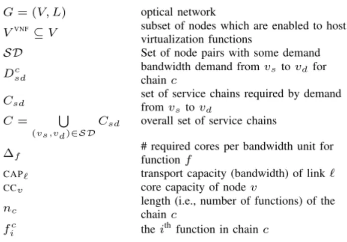
We consider a SDN network that is represented by a graph G = (V, L) where V represents the set of nodes and L the set of links. Each service chain c is defined as an ordered sequence of Virtual Network Functions (VNFs), with some functions possibly repeated. We denote by nc the number of
functions in c, i.e., the length of the sequence. Let C be the set of all service chains.
Demand is defined by a set of requests, where each request is characterized by a source vs, a destination vd, a service
chain c and a bandwidth requirement, i.e., Dc
sd units. Let SD
the set of node pairs with some demand.
Let F be the set of network virtual functions, indexed by f. The amount of (fractional) cores required by function f in any chain is equal to f per unit of bandwidth. Consequently,
Dc
sd⇥ fc
i represents the number of (fractional) cores for
request (vs, vd, c, Dcsd) at the node hosting function fic, the
ith function of chain c. Note that the number of cores that a
G = (V, L) optical network VVNF
✓ V subset of nodes which are enabled to hostvirtualization functions SD Set of node pairs with some demand Dc
sd
bandwidth demand from vsto vdfor
chain c
Csd set of service chains required by demandfrom v sto vd
C = S
(vs,vd)2SD
Csd overall set of service chains
f # required cores per bandwidth unit forfunction f
CAP` transport capacity (bandwidth) of link `
CCv core capacity of node v
nc length (i.e., number of functions) of thechain c
fic the ithfunction in chain c
TABLE II: Notations.
node possesses and that it uses is integral in the model, but cores can be shared by several demands or functions, using a fractional amount of cores.1
We assume that only a subset of nodes VVNF
✓ V can host VNFs. Indeed, deployment of VNFs can be made on general purpose servers or standard IT platforms like high-performance switches, service, and storage, see, e.g., [3] for more details. Running a VNF requires a certain amount of resources2, e.g.,
CPU, memory, disk, while the amount of required resources usually depends on the volume of traffic that passes through it. Efficient scheduling algorithms are indeed required in order to take care of the VNF scheduling and the latency requirements of the requests once the mapping of VNF on virtual nodes is done, see, e.g., [4, 5], but goes beyond the scope of this study. Consequently, each node v 2 VVNF has a given core capacity
CCv. Similarly, each link ` of the network has a transport
capacity CAP`. A summary of the notations can be found in
Table II.
The Service Function Chain Provisioning Problem can be formally stated as follows. For a given demand D, where each individual demand is characterized by a 4-tuple (vs, vd, c, Dcsd), identify the best function locations in order
to both provision the set C of SFCs and demand D, while minimizing the overall bandwidth requirement subject to the core and transport capacities (as expressed by CAP` for the
links and by CCv for the nodes), and optionally to a limit on
the number of NFV nodes and SFC replicas.
When provisioning SFCs, each chain is assigned a path in which functions of c are encountered in the same order as in c, with some functions possibly located at the same node. B. Layered Graph
Following a similar idea as in [6], we use a layered graph GL in order to integrate the search of the function location 1The complexity of a function may not always scale linearly with the unit of
bandwidth of the function. We made this assumption to simplify the model and experiments. In fact, we could easily change the model to take into account other complexity models, such as constant or any linear function (or any function which has a linear approximation).
2We did not consider cases with correlated VNF replicas or synchronization
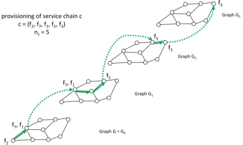
within the search of a route for each connection. GLis defined
as follows. The initial network graph G is transformed into a layered graph GL by adding max
c2C nc layers to graph G
(counting G as the base layer, i.e., layer 0), and where each layer is an exact copy of the original graph G. For every node v 2 V , let vi be the corresponding node in the ith layer
(i = 1, . . . , nc). Every (i 1, i) layer pair is connected by
vertical links from vi 1to vi, see Figure 1 for an illustration.
Finding a path and a chain placement for a request (vs, vd, c, Dcsd) consists in finding a path from node vs on
the first layer to node vd on the (nc+ 1)th layer. Indeed, each
layer represents the progression of the chain, e.g., being on the second layer means that the first function of the chain is already executed. The placement of the node is given by the link used to switch between layers.
All Integer Linear Programming (ILP) models presented in Section IV use the layered graph.
III. RELATED WORK
Following the NFV initiative in 2012 [7], several surveys are now available on NFV, see, e.g., [3, 8, 9] where the various NFV challenges are discussed.
Several works propose partial and exact mathematical formulations for the SFC provisioning problem. Researchers consider different objective functions. Note that some work study the SFC provisioning problem using game theory [10] or approximation algorithms [11, 12, 13].
Hybrid mathematical formulations. In Martini et al. [14] and Riggio et al. [15], the authors only solve the placement and routing for each request independently. A heuristic based on an ILP is proposed in Gupta et al. [16]. The authors only consider the k-shortest paths for every request in the network and a simplified node capacity constraint, for which only one function per node can be deployed. There has been a recent attempt with a column generation model, using a different decomposition than the one proposed in this paper, by [17, 18]. Unfortunately, as the resulting column generation model was not well scaling, its ILP solution is not exact. Exact mathematical formulations. Luizelli et al. [19] provide an exact model minimizing the number of instances of functions in the network. However, they consider only a couple of tens of requests. Savi et al. [20] propose an exact formulation in which the number of VNF nodes is minimized. Their model takes into account additional costs inherent to multi-core environment. However, they only provide results on a small network. In Bari et al. [21], the authors consider the operational expenditure (OpEx) for a daily traffic scenario as their objective function. Mohammadkhan et al. [22] propose an exact model along with heuristics aiming at minimizing the maximum usage of CPU and links. The scope of the experiments is limited to the case in which the number of cores per service is limited to one.
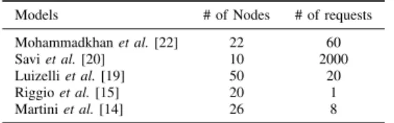
The ILPs proposed in the literature do not scale for large networks. We report the size of the instances they solve
Models # of Nodes # of requests Mohammadkhan et al. [22] 22 60 Savi et al. [20] 10 2000 Luizelli et al. [19] 50 20 Riggio et al. [15] 20 1 Martini et al. [14] 26 8
TABLE III: Maximum topology size and number of requests solved in a reasonable amount of time for models found in the literature.
in Table III. We can observe that they are rather small in comparison with the ones we used in our computational results, see Section VII. To the best of our knowledge, using column generation, our work is the first to optimally solve the problem of SFC placement in a network with 50 nodes and for all-to-all demand scenarios (10,000 requests). This model has been extended to propose energy efficient solutions in [23] and to support failure protection in [24]. Even tough some works [20, 19] minimize the number of function replications in the network, we are also the first to consider constraints on the number of function replications throughout the whole network while minimizing bandwidth usage.
IV. OPTIMIZATIONMODELS
We first present a compact Integer Linear Program (ILP) model, called NFV ILP, in Section IV-A and then a reformu-lation with a Column Generation (CG) decomposition model, called NFV CG, in Section IV-B.
A. Model NFV ILP
Model NFV ILP is a compact Integer Linear Program based on the layered graph described in Section II-B.
Variables. Model NFV ILP uses two sets of variables. The first set is a set of 0-1 variables 'sd,c,i
` defined as follows.
Variable 'sd,c,i
` = 1 if the route of (vs, vd, c, Dcsd) goes
through link ` at layer i in the layered graph GL, 0 otherwise.
The second set corresponds to 0-1 variables ↵sd,c,i
v such that
↵sd,c,i
v = 1if fic is installed on node v. Note that we will use
the convention that if v 62 VVNF, ↵sd,c,i v = 0.
Objective. Minimization of the bandwidth requirements
min X (vs,vd)2SD X c2Csd Dsdc X `2L nc X i=0 'sd,c,i` . (1)
Constraints. There are three sets of constraints.
Flow constraints. They translate the requirement of a path from source to destination going through the locations of the functions of the service chain requested by each node pair demand. Only the source node on the first layer and the destination node on the last layer can have a positive outgoing and incoming flow, respectively. Let !+(u)and ! (u) denote
Graph G = G0 Graph G1 Graph G3 Graph G2 provisioning of service chain c c = (f2, f7, f1, f5, f3) nc= 5 f2 f3 f5 f7, f1 f7, f1 f5 f3
Fig. 1: Layered Graph
the set of outgoing and incoming links of node v, respectively. X `2!+(u) 'sd,c,i` X `2! (u) 'sd,c,i` + ↵sd,c,i v ↵sd,c,i 1v = 0 v2 V, (vs, vd)2 SD, c 2 Csd, 0 < i < nc (2) X `2!+(v) 'sd,c,0` X `2! (v) 'sd,c,0` + ↵sd,c,0v = ⇢1 if v = v s 0 else (vs, vd)2 SD, v 2 V, c 2 Csd (3) X `2!+(v) 'sd,c,nc` X `2! (v) 'sd,c,nc` ↵sd,c,ncv = ⇢ 1if v = vd 0 else (vs, vd)2 SD, v 2 V, c 2 Csd. (4)
Link capacity. Usage of a given link ` is distributed over the different layers of graph GL and cannot exceed the link
transport capacity CAP`.
X (vs,vd)2SD X c2Csd Dcsd nc X i=0 'sd,c,i` CAP` `2 L. (5)
Node capacity. The placement of a function in node v is described by the usage of cross-layer link (vi 1, vi). The usage
of a node is determined by the set of links that are used to move from one layer to the next, and should not exceed its core capacity. X (vs,vd)2SD X c2Csd nc X i=0 fc iD c sd↵sd,c,iv CCv v2 VVNF. (6) B. Model NFV CG
As we will see in Section VII-C, the NFV ILP model does not scale well for medium to large networks because of its very large number of variables 'sd,c,i
` and ↵sd,c,i: L ⇥ SD ⇥
|C|⇥|F |. We thus propose an alternate model, called NFV CG model, with a single set of variables. The NFV CG model relies on the concept of configurations, where a configuration is defined by a potential path provisioning, called service path in the sequel, which is next described formally below for a given request.
A Service Path for request (vs, vd, c, Dcsd)is defined by: (i)
a network path, i.e., an ordered set of nodes from the source to the destination node of the request, and (ii) a set of node locations for the VNFs in the SFC request. Each Service Path is thus specific to a given request and its SFC. However, a given SFC may be shared by several requests.
We use the following additional parameters. Parameters
• p 2 Pc
sd: Service Path from vsto vd, where Psdc denotes
the set of paths from vs to vd for chain c. A service
path is composed of a path in the network and a set of function locations (v, fc
i), identifying the node location
of the functions in the chain. • apiv2 {0, 1}, where a
p
iv= 1if fic is installed on node v
for Service Path p 2 Pc sd.
• `p 2 N denotes the number of occurrences of link ` in
path p. Variables
• ysd,c
p 0, where ysd,cp = 1if request (vs, vd, c, Dcsd) is
forwarded through service path p, 0 otherwise. Objective min X (vs,vd)2SD X c2Csd X p2Pc sd Dcsd X `2L p ` y sd,c p (7)
As for Model NFV ILP, the objective is to minimize the amount of bandwidth used in the SDN network. For a path, this amount is its number of hops, multiplied by the bandwidth requirement of the request. The set of constraints can then be expressed as follows.
Constraints
Exactly one path per demand and per chain: X
p2Pc sd
ysd,cp = 1 c2 Csd, (vs, vd)2 SD. (8)
Link capacity: for all ` 2 L, X (vs,vd)2SD X c2Csd X p2Pc sd (Dc sd `p)⇥ ysd,cp CAP`. (9)
Node capacity: for all v 2 VVNF,
X (vs,vd)2SD X c2Csd nc X i=0 X p2Pc sd fc iD c sda p iv⇥ypsd,cCCv. (10) V. SOLUTIONSCHEME
Model NFV ILP can be easily solved by an ILP solver such as Cplex. Model NFV CG requires more attention as, at first look, it has an exponential number of variables. Indeed, its linear relaxation can be solved exactly using column generation ([25]), using a limited number of configurations, i.e., variables. An integer solution is next derived, together with its accuracy. Details are given below.
A. Generalities on Column Generation
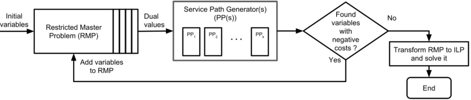
The Column Generation solution scheme requires a decom-position model, called Master Problem (M), which combines the use of the so-called Restricted Master Problem (RMP), i.e., MP with a very small subset of configurations/columns, and the so-called Pricing Problem (PP), i.e., a configuration generator. Consequently, the Restricted Master Problem corresponds to (7) - (10) with a very limited number of variables. Its role is to select the best provisioning, one for each request, while the pricing problem generates improving configurations, i.e., configurations such that, if added to the current RMP, improves the value of its linear relaxation.
The column generation algorithm is depicted in Figure 2. RMP and PP are solved alternately until the PP is unable to generate any new improving configuration/service path, for any request. In such a case, the optimal solution of the linear relax-ation of Model NFV CG has been reached, and we derived an ILP solution, using an ILP solver on the last RMP. Accuracy of the ILP solution is measured by " = (˜zILP z?LP)/z?LP,
where z?
LPis the optimal value of the LP (Linear Programming)
relaxation, and ˜zILP denotes the value of the ILP solution.
B. Pricing Problem
The role of the Pricing Problem is to generate a valid Service Path for a given request. Once again, the formulation relies on the layer graph (GL) introduced in Section II-B. Its objective is
defined by the so-called reduced cost (see [25] if not familiar with linear programming concepts).
• u(j)represents the vector of dual variables of constraints
(j)in the RMP. Note that these values are given as input to the pricing problem in the column generation solution process.
Variables: • ↵i
v 2 {0, 1}, where aiv= 1if fic is installed on node v,
0 otherwise. • 'i
` 2 {0, 1}, where 'i` = 1 if the flow forwarded on
link ` on layer i, i.e., links in each layer in graph GL, 0
otherwise.
The service path generator (pricing problem) is written for each request (vs, vd, c, Dcsd). min X `2L nc X i=0 'i`⇥ (Dcsd+ Dsdc u(9)` ) u(8)sd+ Dcsd X v2V u(10)v nc X i=0 fc i↵ i v. (11)
Flow conservation: they correspond to flow constraints (i.e., route) from the ith function to the (i + 1)th function of the service chain associated with the vs vd request for which
the pricing problem is solved (constraints (12)), and then flow constraints from the source node to the location of the first function of the service chain (constraints (13)), and similarly from the location of the last function of the service chain to the destination node (constraints (14)). Note that ai
v = 0for
all nodes that are not VNF capable. Observe that the next set of constraints takes care of the possibility that several VNFs can be located on the same node, including on the source or destination nodes. X `2!+(v) 'i ` X `2! (v) 'i `+ ↵vi ↵i 1v = 0 v2 V, 0 < i < nc (12) X `2!+(v) '0` X `2! (v) '0`+ ↵0v = ⇢ 1if v = vs 0else v2 V (13) X `2!+(v) 'nc` X `2! (v) 'nc` ↵ncv = ⇢ 1 if v = v d 0 else v2 V. (14) Link capacity. For ` 2 L,
Dsdc nc
X
i=0
Restricted Master Problem (RMP) Initial
variables Dual values
Service Path Generator(s) (PP(s)) PP1 PP2 PPk Transform RMP to ILP and solve it Found variables with negative costs ? No Yes End Add variables to RMP
Fig. 2: Description of the column generation algorithm.
Node capacity. For v 2 VVNF,
nc X i=0 ( fc iD c sd)⇥ ↵ivCCv. (16)
Note that, since the solutions of the pricing problems for all re-quests are independent, we solve in parallel the corresponding ILPs to reduce the overall computational time.
Speeding the solution of the pricing problem with Dijkstra algorithm. As discussed above, the pricing problem can be solved using an ILP. However, it can be solved more quickly using the observationthat it is equivalent to a constrained shortest path in the layered graph. The weight wi` of the link
` at layer i is equal to
wi`= Dsdc + u(9)` D c sd,
and the weight of the link going from layer i to layer i + 1 at node v is equal to
wiv = Dcsdu(10)v fc
i.
Without the capacity constraints, the pricing problem becomes a simple shortest path problem. Since the dual values of the constraints (9) and (10) cannot be negative, we use the Dijkstra algorithm to solve it. If we obtain unfeasible paths, i.e., if they use more capacity than available, they should be discarded, and the pricing problem should be solved again with the capacity constraints. In such a case, we then either solve the ILP formulation of the pricing problem, or use a shortest path dynamic programming algorithm with resource constraints, see, e.g., [26]. By limiting the number of solutions with capacity constraints, we are able to speed up the column generation process, as shown in the next section.
VI. LIMITINGFUNCTIONREPLICAS
We now consider the case in which an operator is limited by the number of replicas of each virtualized function. Such scenario may occur when the operator has a limited budget for its license cost or when the licenses provided for a function only allow a certain number of replicas in the network.
Having a limited number of preset NFV capable nodes, as done in Section VII-D, is a simple addition to the models. However, limiting the number of function replicas, which may be placed on any node, increases greatly the complexity of the
models and the computational times. Indeed, this introduces a large number of binary variables in the model.
In Section VI-A, we provide again two models, the first one is an ILP and the second one uses a column generation decomposition. As the complexity of the second model is high, we introduce in Section VI-B a heuristic algorithm to solve the problem for large networks. The heuristic first finds a good placement of the network functions by solving a variant of a capacitated k-mean clustering problem (or facility location problem) using an ILP, and then uses this placement in the CG model to find a solution of the problem without replicas limit, by constraining the function placement.
A. Models
The models are extensions of NFV ILP and NFV CG, as described below, and are called NFV ILP+ and NFV CG+,
respectively. In both new models, we introduce a new set of variables, bvf, indicating if function f is installed on node v.
We can now limit the total number of functions in the network using the following constraints in both models.
X
v2VVNF
bvf Lf f 2 F, (17)
where Lf represents the maximum number of replicas of
function f.
In the NFV ILP+ model, we then limit the placement of
functions for every request with the following constraints: asd,c,iv bvfc
i v2 V
VNF, (v
s, vd)2 SD,
c2 Csd, 0 < i < nc. (18)
In the NFV CG+ model, a Service Path can only be used
if all the locations where its functions are executed have the corresponding function installed. In other words, a function f must be installed at the location v, i.e., bvf = 1, if any service
path using this location to execute the function f is used. This can be expressed using the following constraints
X c2Csd X (vs,vd)2SD X p2Pc sd p vfy sd,c p Mbvf v2 VVNF, f 2 F, (19) where M |SD| ⇥ |C| and vfp = 1 if function f needs to
Since P p2Pc sd p f vypsd,c P p2Pc sd ysd,c p = 1, we can eliminate
the M constant at the expense of a higher number of con-straints. Constraints (19) are then rewritten:
X p2Pc sd p vfypsd,c bvf v2 VVNF, f2 F, c2 Csd, (vs, vd)2 SD. (20) Pricing Problem
We introduce the set of variables vf into the Pricing
Problem to keep track of the function placement. Note that chains can contain multiple occurrences of the same function, and that this is the purpose of variables ↵vfc
i, allowing a
function to intervene several times (e.g., firewall application) in a service chain, and to be run in different locations, i.e., potentially a different one for each occurrence.
The objective function of the Pricing Problem for a given request (vs, vd, c, Dsdc )for NFV CG becomes:
min X `2L nc X i=0 'i`⇥ ⇣ Dsdc Dsdc u(9)` ⌘ u(8)sd+ Dsdc X v2VVNF u(10)v nc X i=0 fc i↵vfic +X v2V X f2F vfu(20)sd,v,f.
As in the RMP formulation, we add the following two sets of constraints for the number of replicas in the network. First, we limit the number of replicas in the network:
X
v2VVNF
vf Lf f 2 F. (21)
Then, we make sure that functions can only be executed on nodes where they are installed:
vfc
i ↵
i
v v2 VVNF, 0 i nc. (22)
Unlike the Pricing Problem of NFV CG, it is not possible to find a solution using the Dijkstra algorithm due to potential multiple occurrences of the same function in chains, and we thus use an ILP solver (e.g., CPLEX) or a resource constrained shortest path algorithm [26] to obtain its solution. Indeed, links between layers in the layered graph give the locations where the functions of a given chain are executed. However, we need to be careful when considering the function locations. Indeed, if all multiple occurrences are run at the same location (i.e., node), only one licence is required. A path algorithm, such as the Dijkstra algorithm, is not able to compute the number of required licences properly: it would keep adding more licences as it would go through the same function location.
B. Heuristics (NFV Algo+)
As shown in Section VII, NFV CG can find quickly near-optimal solutions to the SFC placement problem, when the number of function replica is not limited. However, NFV CG+
has a much longer execution time and is not able to solve data instances using a large network such as Germany. Thus, we propose a heuristic solution using NFV CG, called NFV Algo+. First, we consider the placement of functions in
the network in the same fashion as a facility location problem, as explained below. Then, we use NFV CG to solve the routing of the requests once the placement has been chosen.
a) Location problem: The core of the method is a variant of a k-mean clustering problem. For each function, we have to choose k = Lf possible locations. As our goal is to
minimize the network bandwidth, a good solution is to choose the locations to minimize the request path lengths, that is the distances between the sources and destinations of the requests and the function locations of the service chains associated with the requests. Our solution is not therefore not exactly a k-mean clustering, but a generalization, as we have link and node capacity constraints to satisfy. We thus model the placement problem as an ILP.
We search for each function f exactly Lf nodes that can
host the function. Since each node has a limited capacity, we also need to consider on which node the function of a specific request must be executed. We thus use the two following sets of variables.
• xsd,cvi 2 {0, 1}, where x sd,c
vi = 1 if the ith function of
chain c for demand (vs, vd)is installed on node v.
• bvf 2 {0, 1}, where bvf = 1 if function f is installed
on v.
The problem is formulated as follows. min X v2VVNF X (vs,vd)2SD X c2Csd X i2{0..nc} :fic=f (d(vs, v) + d(vd, v))⇥ xsd,cvi . (23)
We want to minimize the distance of the route of each request to the location of the functions (23). The distance is given by the sum of the distance to the source, d(vs, v), and the distance
to the destination, d(vd, v). X v2VVNF xsd,cvi = 1 (vs, vd)2 SD, c 2 Csd, 0 i nc, f = fic (24) bvfc i x sd,c vi (vs, vd)2 SD, c 2 Csd, 0 i nc, v2 VVNF, f = fc i. (25)
The functions of a request need to be executed on exactly one node (24) and they can be executed only on nodes on which the function is installed (25).
X (vs,vd)2SD X c2Csd X i2{0..nc}:fc i=f ( fc iD c sd)⇥ x sd,c vi CCv v2 VVNF (26) X v2VVNF bvf Lf. (27)
Finally, we have the node capacity (26) and the maximum license constraints (27).
VII. NUMERICALRESULTS
In this section, we report the numerical results. First, we describe the data sets we used (Section VII-A). Then, we present the performance of NFV CG in Section VII-B. Next, in Section VII-C, we compare the performance of the two models described in Section IV and look at the compromise between the number of VNF nodes and the bandwidth require-ments in Section VII-D. Finally, we compare the different solutions we propose for the case with a limited number of possible VNF replicas and study the impact on bandwidth requirement in Section VII-E.
The computer we use for running the experiments is equipped with an Intel(R) Xeon(R) CPU W5580 @ 3.20GHz and 64GB of RAM.
A. Data Sets
To emulate a realistic traffic, we used the data in [27] in conjunction with the four chains presented in Table IV as in [20]. Each SFC is composed of a sequence of network virtual functions and requires a specific amount of bandwidth. We use the distribution of traffic from [27] to know the number of requests of each service type. For example, a 1TB network load is composed of 699GB of Video Streaming. This amount of traffic correspond to an equivalent of 699
4⇥ 10 3 requests. We
then choose at random the source and destination for each request and then aggregate the resulting set of requests with respect to their source and destination nodes. Overall, we have a total of 4 ⇥ n2 demands (all types of chains for every node
pair).
Service Chain Chained VNFs rate % traffic Web Service NAT-FW-TM-WOC-IDPS 100 kbps 18.2%
VoIP NAT-FW-TM-FW-NAT 64 kbps 11.8% Video Streaming NAT-FW-TM-VOC-IDPS 4 Mbps 69.9% Online Gaming NAT-FW-VOC-WOC-IDPS 50 kbps 0.1%
TABLE IV: Service chain requirements [20]
When choosing the set of nodes which can host VNFs, we select the nodes based on their betweenness centrality, which is the number of paths going through the node, when considering the shortest paths between all pairs of nodes. Betweenness centrality is a good indicator of the importance of a node in the network. Programs were tested on three different networks, whose characteristics are described in Table V.
B. Performance of Model NFV CG
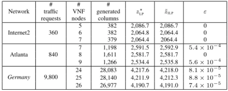
Table VI summarizes the performance of Model NFV CG. We present results for the 3 different topologies for a selected number of VNF nodes, for about half the size of networks. For each instance, we simulate an overall traffic of 1 Tbps.
In the last three columns, we give the optimal value of the linear relaxation (z?
LP), the value of the ILP solution (˜zILP) and
the accuracy of the ILP solution ". In most instances, " = 0, meaning that we obtain the optimal ILP solution. For the cases where " > 0, its value remains very small, meaning that ˜zILP
is very close to the optimal ILP value.
Network Ref. |V | |L| Internet2 [28] 10 16 Atlanta [29] 15 44
Germany 50 88
TABLE V: Network Data
Lastly, we observe that the number of generated columns is fairly small in order to reach very accurate ILP solutions, taking into account that we need to select one column per request, i.e., 360, 840 and 9,800 columns for data instances associated with networks Internet1, Atlanta, and Germany, respectively.
# # #
Network traffic VNF generated z?
LP ˜zILP "
requests nodes columns
Internet2 360 56 382382 2,086.72,064.8 2,086.72,064.4 00 7 379 2,064.4 2064.4 0 Atlanta 840 7 1,198 2,591.5 2,592.9 5.4⇥ 10 4 8 1,611 2,581.7 2,581.7 0 9 1,266 2,534.4 2,535.8 5.6⇥ 10 4 Germany 9,800 24 28,083 4,217.6 4,218.0 8.1⇥ 10 5 25 28,140 4,211.9 4,212.3 8.8⇥ 10 5 26 26,977 4,190.7 4,191.0 7.4⇥ 10 5
TABLE VI: Numerical results
C. Comparison ILP vs CG
In Figure 5, we compare the two models presented in Section IV on the Germany network. We also compare the computational times for NFV CG when the Pricing Problem is solved using CPLEX and Dijkstra. We assume all nodes are VNF enabled nodes and the number of requests varies between 10 and 100% of the requests in an all-to-all traffic scenario.
Model NFV ILP is solved exactly using the CPLEX ILP solver, while Model NFV CG is solved using the solution scheme described in Section V, i.e., with an "-optimal solution scheme. As the accuracy of the solutions of Model NFV CG is very good, the solutions of both models are identical. However, NFV ILP takes more time as the number of requests increases. Indeed, when reaching 90% requests in the all-to-all scenario, NFV ILP takes more than one hour to find the optimal solution and does not provide a solution in less than a day for 100%. Comparatively, NFV CG outputs an "-optimal solution with all requests in two minutes and a half. Using Dijkstra, the solution is found in 8 seconds. See Figure 5 for the comparison of computing times, using the ratio of the computational times.
D. Bandwidth Requirement and Delay vs. Number of VNF Capable Nodes
In this set of experiments, we want to study the impact of the number of VNF nodes on the bandwidth requirement and the delay. Generating numerous VNF nodes could be quite costly (e.g., license price, CPU utilization, energy consumption), and should be compensated by a significant decrease in the bandwidth requirement or justified by unacceptable delays otherwise. Our results show that this is not the case. We next discuss them in detail.
(a) Internet2 (b) Atlanta (c) Germany
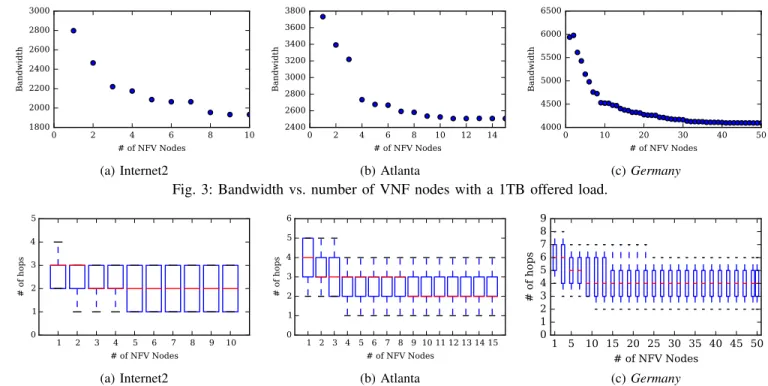
Fig. 3: Bandwidth vs. number of VNF nodes with a 1TB offered load.
(a) Internet2 (b) Atlanta (c) Germany
Fig. 4: Distribution of the number of hops for each demand vs. number of VNF nodes with a 1TB offered load. Boxes are defined by the first and third quartiles. Ends of the whiskers correspond to the first and ninth deciles.
Fig. 5: Computational times of NFV ILP and NFV CG on the Germany network. NFV ILP does not provides results for 80% and up in a reasonable time.
Figure 3 shows the bandwidth used for an overall 1Tbps traf-fic when the number of VNF nodes varies. As we allow more VNF nodes, the overall required bandwidth in the network decreases. This is as expected. Since every request requires a SFC, their provisioning must go through VNF nodes in the required order, possibly requesting more hops than in one of the shortest paths in the network. However, what we learn from Figure 3 is that, when reaching 50% for VNF capable nodes, the bandwidth gain is getting significantly smaller.
We next investigated the increase of the number of VNFs
with respect to the number of hops. Results are described in Figure 4 using a box-and-whisker plot. It shows that the median value for the number of hops stabilizes as soon as the number of VNF nodes reaches 3, 9, 9 for the Internet2, Atlanta and Germany networks, respectively. While the stabilization occurs later with bandwidth requirements, these results say that, indeed, only a few requests are affected when increasing the number of VNFs beyond the 3, 9 and 9 values for Internet2, Atlanta and Germany networks, respectively. Consequently, for homogeneous traffic as in our experiments, there is little advantage both in terms of number of hops and bandwidth requirements to increase much the number of VNF nodes. It might be slightly different with heterogeneous traffic.
E. Limited Number of Function Replicas
We now evaluate the three methods proposed for a limited number of function replicas, NFV ILP+, NFV CG+ and the
heuristic algorithm NFV Algo+. We consider the scenarios
presented in Section VII. All nodes can potentially host VNFs. We first present the execution times and then the evolution of the bandwidth usage as a function of the number of allowed function replicas.
a) Execution Times: We provide in Figure 6 the execution times of the NFV ILP+, NFV CG+, and of NFV Algo+ for
the Internet2, Atlanta, and Germany data sets.
We first observe that, as expected, the more stringent the constraint on the number of function replicas, the harder it is for the methods to find a solution. For Internet2, NFV CG+
only takes a few seconds to propose a solution when the number of replications is 10 (equal to the number of nodes), 9
(a) internet2 (b) atlanta (c) Germany
Fig. 6: Execution times of the three methods, the ILP, the column generation model, and the algorithm NFV Algo+, for different
limits on the number of function replicas.
or 8. However, more than 1 day is necessary to solve the case in which the number of allowed replications is 4. NFV ILP+
and NFV Algo+ experience a similar trend, for lower order
of execution times (respectively between 4 s and 1 min and between 400 ms and 4 s).
The second observation is that the execution time of NFV ILP+ becomes almost prohibitive (more than 1 day)
when the number of allowed function replications is small. In fact, we were not able to run NFV ILP+ for networks larger
than Internet2. On the contrary, NFV CG and NFV Algo+
have low execution times for any number of replications. Considering larger networks, NFV ILP+ runs on Atlanta for
any number of replicas, but not on Germany, for which, only NFV Algo+ provides solutions.
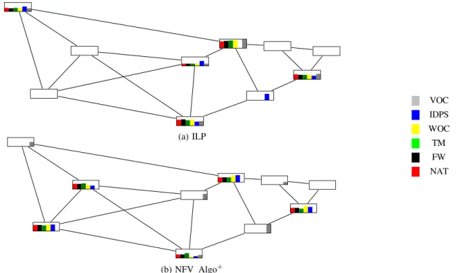
b) Replica Placement: We provide the results of the function replica placement in Figure 7 for Internet2 and in Figure 8 for Germany. For each node and for each function, we present the percentage of requests associated with the function replica. A value of 0 means that there is no function replica on the node. The height of the box is set to the maximum value over all nodes, respectively 36% for Internet2 and 20% for Germany. For Internet2, the maximum number of function replicas was set to 5. We compare the result of the first phase of NFV Algo+ (placing function replicas) to the one of the
ILP. We observe that the optimal solution provided by the ILP has selected 5 nodes (only a replica of the IDPS function is in another node), which are central in the network. This confirms the intuition that this kind of nodes are good candidates, as they have a small average distance to the other nodes, which are sources and destinations of requests. This intuition is at the core of NFV Algo+ first phase, which selects a set of nodes
minimizing the distances between the sources and destinations of the requests and the replica positions. NFV Algo+ also
selected 5 nodes (only 4 replicas of the VOC function are in 4 other nodes). Three of them are common with the ILP, and two are different. The two last ones seem less central, but they have a high degree, which reduces their distances to the other nodes.
For Germany, the number of function replicas was limited to 11. Only the result of NFV Algo+ is presented as the ILP
does not run on the network. We observe that mostly central nodes with often a high degree are selected. Indeed, again, they
are nodes with a small average distance to the other nodes, and thus are good candidates for function replicas. We thus validate NFV Algo+, which provides good solutions to the placement
problem. We now study the bandwidth usage.
c) Bandwidth Usage: Figures 9a, 9b and 9c show the bandwidth usage respectively for Internet2, Atlanta, and Ger-many. The number of allowed replications varies between n and 1, where n is the number of nodes in the network. The results are given using NFV Algo+ (and additionally using
ILP for Internet2). To assess the quality of the solutions, we compare the results given using NFV Algo+with the results of
the relaxation of NFV CG+, which constitutes a lower bound
on the optimal solution. The gap for NFV CG+ is higher
than the one of NFV CG. The reason is that the limitation on the number of replicas requires the introduction of new constraints, which are hard to relax efficiently3. However, the
gap is within few percent for most of the values. For small number of replicas, the gap is higher. However, the difference to optimal can be a lot smaller than the gap. For instance, for Internet2, we see that the largest gap is around 20%, when the difference to optimal given by NFV ILP+ is only 4%. To
summarize, the solutions given by NFV Algo+are within few
percent from optimal for most values (and 16% for the worst case) and for the three networks. This shows that NFV Algo+
provides good solutions.
First, we need at least 4, 4, and 11 function replicas for Internet2, Atlanta and Germany, respectively. We observe a general trend for the three networks. Starting from n, there is a first phase in which the number of function replications can be reduced without affecting significantly the bandwidth usage. This first phase corresponds to values between 10 and 6 for Internet2, 15 and 7 for Atlanta, 50 and 20 for Germany. In a second phase, on the contrary, the number of function replications can be reduced only at the cost of a strong increase of bandwidth usage: from 1,932 to 2,392 (+24%) for Internet2, from 2,506 to 2,974 (+19%) for Atlanta, from 4,095 to 4,860 (+19%) for Germany. Another way to state it, as a takeaway for a network operator: having a few more replicas than necessary leads to important gains, when adding further supplementary
3Note that, when the number of replicas is small for Germany, the relaxation
(a) ILP (b) NFV Algo+ NAT FW TM WOC IDPS VOC
Fig. 7: Placement of functions given by the ILP (a) and by NFV Algo+ (b) when the number of function replicas is limited to
5 for Internet2. Bar height in a node gives the percentage of requests (between 0 and 36%) associated with the node function replica.
replicas has less impact.
F. Random Topologies
To assess the impact of network parameters such as topology size in terms of number of nodes and links, traffic load and demand heterogeneity, we now focus on random instances.
Instance generation. We generate random networks using two parameters: the number of nodes n and the edge density p. Starting from a random tree of size n, we add a link between each unconnected pair of nodes with a probability p. Once a graph is generated, we create a traffic matrix similarly to Section VII-A. For a given load L, we generate a request by choosing at random a pair of nodes and a random service until the sum of the load over all the requests is equal to L. We then aggregate requests with the same source, destination and service chain.
We consider uniform and non-uniform traffic. We generate uniform traffic by selecting each pair of nodes uniformly at random. For non-uniform traffic, we introduce a population and distance model [30]. We generate the population of the network nodes according to a power law distribution with parameter ↵. The population of the i-th node is proportional to by 1/ i↵. The probability to chose a pair of nodes (u, v) is
then given by (Pu⇥ Pv)/ Duv, where Pu is the population
of u and Duv is the distance in number of hops between u
and v.
Finally, to generate the service chains, we vary the number of chains (nc), the number of functions (nf) and the size
of the chains sc. We build nc chains by choosing uniformly
at random sc functions in the set of nf functions. We then
associate a bandwidth requirement (in kB) to each chain uniformly at random in the range [50, 4096]. We also consider the service chains presented in Section VII-A.
Experiments. We consider two metrics here: the minimum required bandwidth as well as the critical number of licenses. We define formally the critical number of licenses as the minimum number of licenses for which the bandwidth required does not exceed ✓% of the bandwidth required without replica limit. We look at different values of ✓: 0, 1, 5, and 10.
Number of nodes. First, we look at the critical number of licenses needed when the number of nodes varies in Figure 10. The critical number of licenses grows linearly with the number of nodes: from 6 licenses with 10 nodes to 13 licenses with 20 nodes when ✓ = 0. Note that the value of ✓ chosen to define the critical number of licenses of course changes the values of the metric, but does not change the global trend observed when varying the network parameters.
Edge density. However, the density of the graph has a higher influence on the number of critical licenses. Indeed, we observe in Figure 11 that a sparse network requires only 5 licenses, but a complete network requires 9 licenses. As the density increases, most of the requests can be routed on one-hop paths. Thus, a slight decrease in the number of licenses can greatly increase the bandwidth required as some requests
NAT FW TM WOC IDPS VOC
Fig. 8: Placement of functions given by NFV Algo+ when the number of function replicas is limited to 11 for Germany. Bar
height in a node gives the percentage of requests (between 0 and 20%) associated with the node function replica
(a) Internet2 (b) Atlanta (c) Germany
Fig. 9: Bandwidth usage as a function of the number of allowed function replicas.
might now be routed on a longer path. These results confirm the findings of Section VII, as ISP (Internet Service Provider) topologies such as those we studied, usually have a low density (e.g., 0.1 for Atlanta and 0.03 for Germany).
Heterogeneity coefficient. As we can see in Figure 12, the higher the difference in population, the lower the critical number of licenses is. When the population is concentrated on a few nodes (for high value of ↵), most of the traffic is between these nodes. Thus, it is easier to cover a significant part of the requests with only a few licenses by selecting nodes in the paths of the largest requests.
Traffic load. In Figure 13, we look at the critical number of
licenses when we vary the traffic load. We vary the total load between 1 GB and 1 TB. We can observe the critical number of licenses is barely impacted by the load of the network. In the same vein, we observed that the impact of the service chains on the critical number of licenses is not noticeable.
In conclusion, the critical number of licenses is mostly impacted by the shape of the network (size and density) as well as the homogeneity of the traffic. The traffic load and the type of services do not have any noticeable impact.
VIII. CONCLUSIONS
In this paper, we look at the Service Function Chain Placement problem and propose two ILP models to solve it.
10 12 14 16 18 20 # Nodes 0 5 10 15 20 C ri ti ca ln um ber of lic en ses 1000 1500 2000 2500 3000 M in im um ba nd w id th req ui red 0% 1% 5% 10% Min. bandwidth
Fig. 10: Critical number of licenses as a function of the number of nodes. (p=0.1, uniform traffic (1TB)).
0.1 0.2 0.3 0.4 0.5 0.6 0.7 0.8 0.9 1.0 Edge probability 0 2 4 6 8 10 C ri ti ca ln um ber of lic en ses 1000 1500 2000 2500 3000 M in im um ba nd w id th req ui red 0% 1% 5% 10% Min. bandwidth
Fig. 11: Critical number of licenses as a function of edge probability (n=10, uniform traffic (1TB)).
0 1 2 3 4 5 6 7 8 ↵ 0 2 4 6 8 10 C ri ti ca ln um ber of lic en ses 1000 1500 2000 2500 3000 M in im um ba nd w id th req ui red 0% 1% 5% 10% Min. bandwidth
Fig. 12: Critical number of licenses as a function of the coefficient of heterogeneity (n=10, p=0.1, 1TB). 100 101 102 103 Load (Gb) 0 2 4 6 8 10 C ri ti ca ln um ber of lic en ses 150 200 250 300 350 400 # D em an ds 0% 1% 5% 10% # demands
Fig. 13: Critical number of licenses as a function of the load (n=10, p=0.1, uniform traffic)
We show that the first compact ILP model does not scale well for large networks. However, with a decomposition model such as Model NFV CG, we can solve exactly the Service Function Chain Provisioning Problem. This leads to a first model that scales with an increasing number of nodes, but also, with an increase of the number of requests with service chain requirements.
We also tackle the bandwidth minimization with a limit on the number of VNF replicas. To this end, we extended our ILP models and proposed an heuristic algorithm based on NFV CG and a capacitated k-mean clustering problem. Using Model NFV CG, we investigated the tradeoff among the network bandwidth requirement, the number of VNF capable nodes, and the limit on the number of VNF replicas. We found out that diminishing returns occur when adding VNF capable nodes, and that, when more than 50% of the network can host VNF, they are only few benefits. A similar tradeoff exists for the number of replicas: when starting from the configurations with the minimum possible number of replicas, adding a small number of them decreases significantly the bandwidth usage, but then adding more replicas shows a little extra gain.
ACKNOWLEDGMENTS
B. Jaumard has been supported by a Concordia University Research Chair (Tier I) on the Optimization of Communication Networks and by an NSERC (Natural Sciences and Engi-neering Research Council of Canada) grant. N. Huin and F. Giroire have been partially supported by ANR program ANR-11-LABX-0031-01 and Mitacs.
REFERENCES
[1] “NFV basics: Implementation, challenges and benefits,” http://searchsdn.techtarget.com/essentialguide/ NFV-basics-A-guide-to-NFV-implementation-challenges-and-benefits, 2016.
[2] “Service chaining in carrier networks,” http://www.qosmos.com/wp-content/uploads/2015/
02/Service-Chaining-in-Carrier-Networks WP
Heavy-Reading Qosmos Feb2015.pdf, February 2015. [3] Y. Li and M. Cheng, “Software-defined network function
virtualization: A survey,” IEEE Access, vol. 3, pp. 2542 – 2553, 2015.
[4] H. Alameddine, L. Qu, and C. Assi, “Scheduling service function chains for ultra-low latency network services,” in 13th International Conference on Network and Service Management (CNSM), 2017, pp. 1–9.
[5] R. Mijumbi, J. Serrat, J.-L. Gorricho, N. Bouten, F. D. Turck, and S. Davy, “Design and evaluation of algorithms for mapping and scheduling of virtual network functions,” in 1st IEEE Conference on Network Softwarization (Net-Soft), 2015, pp. 1–9.
[6] A. Dwaraki and T. Wolf, “Adaptive service-chain routing for virtual network functions in software-defined net-works,” in Workshop on Hot topics in Middleboxes and Network Function Virtualization (HotMIddlebox), 2016, pp. 32–37.
[7] A. Gember, P. Prabhu, Z. Ghadiyali, and A. Akella, “To-ward software-defined middlebox networking,” in ACM Workshop on Hot Topics in Networks (HotNets), 2016, pp. 7–12.
[8] J. Herrera and J. Botero, “Resource allocation in NFV: A comprehensive survey,” IEEE Transactions on Network and Service Management, vol. 13, no. 3, pp. 32–40, March 2016.
[9] R. Mijumbi, J. Serrat, J.-L. Gorricho, N. Bouten, F. D. Turck, and R. Boutaba, “Network function virtualization: State-of-the-art and research challenges,” IEEE Commu-nications Surveys & Tutorials, vol. 18, no. 1, pp. 236 –262, 2016.
[10] S. D’Oro, L. Galluccio, S. Palazzo, and G. Schembra, “Exploiting congestion games to achieve distributed ser-vice chaining in nfv networks,” IEEE Journal on Selected Areas in Communications, vol. 35, no. 2, pp. 407–420, Feb 2017.
[11] R. Cohen, L. Lewin-Eytan, J. S. Naor, and D. Raz, “Near optimal placement of virtual network functions,” in Proceedings of IEEE INFOCOM, 2015.
[12] Y. Sang, B. Ji, G. R. Gupta, X. Du, and L. Ye, “Provably efficient algorithms for joint placement and allocation of virtual network functions,” in Proceedings of IEEE INFOCOM, 2017.
[13] A. Tomassilli, F. Giroire, N. Huin, and S. P´erennes, “Provably efficient algorithms for placement of service function chains with ordering constraints,” in IEEE In-ternational Conference on Computer Communications (INFOCOM), Honolulu, Hawai, US, 2018.
[14] B. Martini, F. Paganelli, P. Cappanera, S. Turchi, and P. Castoldi, “Latency-aware composition of virtual func-tions in 5G,” in IEEE Conference on Network Softwariza-tion (NetSoft), 2015, pp. 1–6.
[15] R. Riggio, A. Bradai, T. Rasheed, J. Schulz-Zander, S. Kuklinski, and T. Ahmed, “Virtual network functions orchestration in wireless networks,” in International Con-ference on Network and Service Management (CNSM), 2015, pp. 108–116.
[16] A. Gupta, M. Habib, P. Chowdhury, M. Tornatore, and B. Mukherjee, “Joint virtual network function placement and routing of traffic in operator networks,” UC Davis, Davis, CA, USA, Tech. Rep., 2015.
[17] A. Gupta, B. Jaumard, M. Tornatore, and B. Mukherjee, “Service chain (SC) mapping with multiple SC instances in a wide area network,” IEEE Global Telecommunica-tions Conference - GLOBECOM, pp. 1–6, 2017. [18] ——, “A scalable approach for service chain (SC)
map-ping with multiple SC instances in a wide-area network,” JSAC, 2018.
[19] M. Luizelli, L. Bays, L. Buriol, M. Barcellos, and L. Gaspary, “Piecing together the NFV provisioning puz-zle: Efficient placement and chaining of virtual network functions,” in IFIP/IEEE International Symposium on Integrated Network Management (IM), 2015, pp. 98–106. [20] M. Savi, M. Tornatore, and G. Verticale, “Impact of processing costs on service chain placement in network functions virtualization,” in IEEE Conference on Network Function Virtualization and Software Defined Network (NFV-SDN), Nov. 2015, pp. 191–197.
[21] M. Bari, S. Chowdhury, R. Ahmed, R. Boutaba, and O. Duarte, “Orchestrating virtualized network functions,” IEEE Transactions on Network and Service Management, vol. PP, pp. 1–1, 2016.
[22] A. Mohammadkhan, S. Ghapani, G. Liu, W. Zhang, K. Ramakrishnan, and T. Wood, “Virtual function place-ment and traffic steering in flexible and dynamic software defined networks,” in IEEE International Workshop on Local and Metropolitan Area Networks, 2015, pp. 1–6. [23] N. Huin, A. Tomassilli, F. Giroire, and B. Jaumard,
“Energy-efficient service function chain provisioning,” J. Opt. Commun. Netw., vol. 10, no. 3, pp. 114–124, Mar 2018. [Online]. Available: http://jocn.osa.org/abstract. cfm?URI=jocn-10-3-114
[24] A. Tomassilli, N. Huin, B. Jaumard, and F. Giroire, “Re-source requirements for reliable service function chain-ing,” in IEEE International Conference on Communica-tions (ICC), Kansas City, Kansas, US, 2018, to appear. [25] V. Chvatal, Linear Programming. Freeman, 1983. [26] S. Irnich and G. Desaulniers, Shortest Path Problems with
Resource Constraints. Boston, MA: Springer US, 2005, pp. 33–65.
[27] Cisco Visual Networking Index: Forecast and Methodol-ogy, 2014–2019, CISCO, May 2015.
[28] “Internet2 network infrastructure topology,” http://www. internet2.edu/media\ files/422, 2014.
[29] S. Orlowski, M. Pi´oro, A. Tomaszewski, and R. Wess¨aly, “SNDlib 1.0–Survivable Network Design Library,” in Proceedings of the 3rd International Network Optimiza-tion Conference (INOC 2007), Spa, Belgium, April 2007, pp. 276–286.
[30] A. Betker, C. Gerlach, R. H¨ulsermann, M. J¨ager, M. Barry, S. Bodamer, J. Sp¨ath, C. Gauger, and M. K¨ohn, “Reference transport network scenarios,” BMBF Multi Tera Net, Tech. Rep., July 2003.
![TABLE I: Middle-Box Functions for Inclusion Into Service Chains [2]](https://thumb-eu.123doks.com/thumbv2/123doknet/13644854.427787/2.918.482.855.560.692/table-i-middle-box-functions-inclusion-service-chains.webp)


![[PDF] Langage JavaScript cours pdf](data:image/gif;base64,R0lGODlhAQABAIAAAP///wAAACH5BAEAAAAALAAAAAABAAEAAAICRAEAOw==)