HAL Id: hal-01685554
https://hal.sorbonne-universite.fr/hal-01685554
Submitted on 16 Jan 2018
HAL is a multi-disciplinary open access
archive for the deposit and dissemination of sci-entific research documents, whether they are pub-lished or not. The documents may come from teaching and research institutions in France or abroad, or from public or private research centers.
L’archive ouverte pluridisciplinaire HAL, est destinée au dépôt et à la diffusion de documents scientifiques de niveau recherche, publiés ou non, émanant des établissements d’enseignement et de recherche français ou étrangers, des laboratoires publics ou privés.
The “Residential” Effect Fallacy in Neighborhood and
Health Studies: Formal Definition, Empirical
Identification, and Correction
Basile Chaix, Dustin Duncan, Julie Vallée, Anne Vernez-Moudon, Tarik
Benmarhnia, Yan Kestens
To cite this version:
Basile Chaix, Dustin Duncan, Julie Vallée, Anne Vernez-Moudon, Tarik Benmarhnia, et al.. The “Residential” Effect Fallacy in Neighborhood and Health Studies: Formal Definition, Empirical Iden-tification, and Correction. Epidemiology, Lippincott, Williams & Wilkins, 2017, 28 (6), pp.789 - 797. �10.1097/EDE.0000000000000726�. �hal-01685554�
1 Type of manuscript: Original Article
The “residential” effect fallacy in neighborhood and health studies: formal definition, empirical identification, and correction
Basile Chaix,a,b Dustin Duncan,c Julie Vallée,d Anne Vernez-Moudon,e Tarik Benmarhnia,f
Yan Kestensg
From:
aInserm, UMR-S 1136, Pierre Louis Institute of Epidemiology and Public Health,
Nemesis team, Paris, France;
bSorbonne Universités, UPMC Univ Paris 06, UMR-S 1136, Pierre Louis Institute of
Epidemiology and Public Health, Nemesis team, Paris, France;
cDepartment of Population Health, New York University School of Medicine, New
York, NY, USA
dUMR Géographie-Cités, CNRS, Paris, France
eDepartment of Urban Design and Planning, Urban Form Lab, University of
Washington, Seattle, WA, USA
fDepartment of Family Medicine and Public Health & Scripps Institution of
Oceanography, University of California, San Diego, La Jolla, USA
gDepartment of Social and Preventive Medicine, University of Montreal, Montreal,
2
Correspondence: Basile Chaix, UMR-S 1136, Pierre Louis Institute of Epidemiology and Public Health, Faculté de Médecine Saint-Antoine, 27 rue Chaligny, 75012 Paris, France. e-mail: basile.chaix@iplesp.upmc.fr.
Running head: The “residential” effect fallacy
Conflicts of Interest and Source of Funding
Conflicts of interest: None declared.
This study was supported by INPES (National Institute for Prevention and Health Education); the Ministry of Ecology (DGITM); Cerema (Centre for the Study of and Expertise on Risks, the Environment, Mobility, and Planning); ARS (Health Regional Agency) of Ile-de-France; STIF (Ile-de-France Transportation Authority); the Ile-de-France Regional Council; RATP (Paris Public Transportation Operator); and DRIEA (Regional and Interdepartmental Direction of Equipment and Planning) of Ile-de-France.
1 Background
Due to confounding from macro-organizations of territories and resulting correlation between residential and nonresidential exposures, classically estimated residential neighborhood-outcome associations capture nonresidential environment effects, overestimating residential intervention effects. Our study diagnosed and corrected this “residential” effect fallacy bias applicable to a large fraction of neighborhood and health studies.
Methods
Our empirical application investigated the effect that hypothetical interventions raising the residential number of services to 200, 500, or 1000 would have on the probability that a trip is walked. Using GPS tracking and mobility surveys over 7 days (227 participants, 7440 trips; Paris region, 2012–2013), we used a multilevel linear probability model estimating the trip-level association between the residential number of services and walking to derive a naïve intervention effect estimate; and a corrected model accounting for residential, trip origin, and trip destination numbers of services to determine a corrected intervention effect estimate (true effect conditional on assumptions).
Results
There was a strong correlation in service densities between the residential neighborhood and nonresidential places. From the naïve model, hypothetical interventions raising the residential number of services to 200, 500, and 1000 were associated with an increase by 0.020, 0.055, and 0.109 of the probability of walking in the intervention groups. Corrected estimates were of 0.007, 0.019, and 0.039. Thus, naïve estimates were overestimated by multiplicative factors of 3.0, 2.9, and 2.8.
2 Conclusions
Commonly estimated residential intervention-outcome associations substantially overestimate true effects. Our paradox-like conclusion is that, to estimate residential effects, investigators critically need information on nonresidential places visited.
3 INTRODUCTION
The present study contributes to the identification and correction of biases due to which commonly estimated associations between neighborhood characteristics and health/behavioral outcomes do not reflect causal neighborhood effects. Classical residential neighborhood studies use regression models to correlate residential exposures with overall health/behavioral outcomes (e.g., cumulating behavior inside and outside the residential neighborhood)1-4 in order to quantify
residential intervention effects. Among the assumptions that need to be met for such associations to represent the target causal effects (see the first section of eAppendix 1 for a tentative overview of these conditions), the counterfactual framework requires the absence of confounding. With confounding, unmeasured factors causally influence both the exposure and the outcome or determinants of the exposure and outcome, threatening the exchangeability between exposure groups required to validly estimate causal effects.5 To improve the quality of causal inference, the
present study aims to describe, diagnose, and correct a major confounding bias applicable to a large fraction of neighborhood and health studies. Surprisingly, this bias has received almost no attention in the literature (eAppendix 2). This source of bias has the major implication that residential neighborhood-outcome associations as commonly estimated may substantially overestimate the effects that residential interventions would have on the health of residents.
Recently scholars have suggested that environmental exposures in the multiple places visited by people may influence health beyond residential neighborhood exposures.6-10 The source of the
“residential” effect fallacy described here is that for many exposures, residential characteristics may be correlated with those of the multiple contexts visited during the daily activities (within-individual correlation), due to a common causal antecedent (see Figure 1).11,12 Consequently,
associations between residential neighborhood and health outcomes as classically estimated may capture some of the effect that nonresidential environments visited may have on behaviors and
4
health (confounding of residential neighborhood–health associations, used for quantifying residential intervention impacts, by nonresidential effects). The “residential” effect fallacy implies that, because of the correlation between residential and nonresidential characteristics and resulting confounding, intervening on the residential neighborhood may not have the effect expected from classically estimated residential neighborhood–health associations.
As an empirical illustration, the present study relied on GPS tracking and on a mobility survey to precisely assess places visited over 7 days.8,13,14 The resulting ability to disentangle truly
residential from nonresidential effects allowed us to demonstrate the existence of a major
generator of confounding that we refer to as the “residential” effect fallacy (we use quotes to put into question the residential nature of the underlying effect), quantify its magnitude, and correct for it. As an illustration, we focus on the well-known hypothesis that the residential accessibility to services fosters transport walking.1,15-17.
METHODS
Data collection and processing
Population
The RECORD Study participants, recruited during preventive health checkups, were born in 1928–1978 and were residing at baseline in 112 municipalities of the Paris Ile-de-France region.18-23 During the second study wave, 410 participants were invited to enter the RECORD
GPS Study (approved by the French Data Protection Authority) in 2012–2013.13 Of these, 247
accepted to participate and signed an informed consent form. Nine participants withdrew from the study and data were incomplete for four participants, resulting in a final completion rate of 57.1% (N = 234). Seven participants who either lived or spent the 7-day follow-up outside the Île-de-France region were discarded. Overall, 227 participants were included.
5
GPS-based mobility survey
Participants wore a QStarz BT-Q1000XT GPS receiver24 on the right hip for the recruitment day
and 7 additional days and filled a travel diary. GPS data (one point every 5 seconds) were processed by an ArcInfo 10 Python script (www.spherelab.org/tools).25 It identified the places
visited by participants (stationary locations) over the data collection period. The algorithm calculates a kernel density surface from the set of GPS points for each participant, extracts peaks as potentially visited locations, derives a timetable of all visits (of at least 10 minutes) over the period to each detected location with their start and end times, and uploads this information in the Mobility Web Mapping application.
The telephone prompted recall mobility survey13,17 was based on this web mapping
application.13 With the participant, using the travel diary, the survey operator confirmed each of
the detected visits to places (where participants fulfill functions) and corresponding trips, geolocated visits to places undetected by the GPS receiver or algorithm (e.g., very short visits), and modified/removed inaccurate/incorrect visits to places. For each visited place, participants reported the type of activity practiced at the location and the transport modes to reach the place. A SAS program generated the succession of visited places and trips between places with their start/end times.13 Over 7 days, the 227 participants made 7440 (potentially multimodal) trips
between places.
Measures
Walking
Based on the survey, a trip-level binary outcome was set to 1 (vs. 0) if only walking was used in the trip (partly walked trips also using, e.g., public transport coded as non-walking trips).
6
Individual covariates
Age (three categories: 35–49; 50–64; ≥65 years) and gender were considered. Marital status was coded as living alone or in a couple. Education was coded in four categories: no education, primary education, or lower secondary education; higher secondary education and lower tertiary education; intermediate tertiary education; and upper tertiary education. Household income per consumption unit was coded in three categories using the tertiles. Employment status was categorized in four classes: stable job; unstable/precarious job; unemployed; and other.
As neighborhood selection factors,6,26 participants were asked whether, before moving to their
current residence, when they were looking for a neighborhood to live, they found it important to live in a neighborhood (i) with good access to public transport and (ii) with enough services and facilities.17 Each item was coded in three categories.
Modes in previous trips
Modes used in previous trips are a major confounder for the association between the trip-level service accessibility and walking.17 Relying on a car in the previous trip influences both the
environment visited and the mode in the next trip. For each trip, we counted the number of trips done since the last visit at home or in an alternative residence. A binary variable indicated whether a bike was used in one of these previous trips. A three-category variable indicated whether a personal motorized vehicle was used in none, some, or all of these previous trips.
Environmental measures
The spatial accessibility to services was computed within street network buffers (radius = 1 km, corresponding to a 10-to-15 minute walk27-29) centered on the departure and arrival of each trip
7
and on the residence (ArcInfo 10.0, Network Analyst). Using the Permanent Database of
Facilities (Insee, 2011), we calculated the number of services of all types (public services, shops, entertainment facilities, etc.; see detail in eAppendix 3) in each buffer.
As illustrated in Figure 2, we calculated the percentage of each trip origin buffer and of each trip destination buffer that overlapped the residential buffer. When the percentage of overlap was 0 < X < 100, we calculated separately the number of services in the part of the trip
origin/destination buffer that overlapped and in the part that did not overlapped the residential buffer.
Statistical analysis and calculations
Analytic sample
We excluded episodes at activity places, yielding a sample of trips. Regression analyses excluded the following trips from the full sample (n = 7440): trips >4 km of length as non-easily walkable (n = 2597); atypical trips (professional tours, etc.) (n = 3); and trips starting and/or ending outside the Ile-de-France region (n = 207). The analytical sample comprised 4633 trips.
Correlation in service accessibility between residential and nonresidential neighborhoods
This correlation is a consequence of the causal structure in Figure 1 and the potential vector of the “residential” effect fallacy. We estimated a multilevel linear regression model with a random effect at the individual level to investigate the relationship between the density of services per km² in the residential buffer (explanatory variable) and the density of services in the trip origin buffer (outcome). Trips starting at the residence were removed from this regression database. Moreover, for trips whose origin buffer partly overlapped the residential buffer, we used as the outcome the density of services per km² in the portion of the trip origin buffer that did not overlap
8
the residential buffer (we used densities per km² in this analysis rather than counts of services as in the main analyses to deal with these portions of buffers). Interactions between the residential density of services and, on the one hand, the street network distance between the residence and the trip origin, and on the other hand the square of this distance (quadratic term), were specified.
General description of the approach
To mimic an intervention focused on poorly served neighborhoods, the hypothetical interventions examined are to raise the number of services accessible in the residential buffer to 200, 500, or 1000 if below that number.
We estimated regression models at the trip level (one observation per trip).13,17 Variations in
the probability of exclusively walking during a trip were modeled with linear probability models (binary variable, identity link). This model quantifies associations on the risk difference scale,30
i.e., on the probability scale, which is particularly relevant to decision-making.31 Multilevel
models were used, with a random effect at the individual level, to account for the within-individual correlation in modal choice. Individual sociodemographic covariates and neighborhood selection factors were forced into the models.
Naïve estimate of the residential intervention effect
The model based on trip-level data to calculate the naïve (biased) estimate of the intervention effect included sociodemographic variables, neighborhood selection factors, and the residential number of services (two continuous variables: linear and quadratic terms). Based on model coefficients, we calculated for each trip the predicted probability that it is entirely walked from all model covariates (including the number of services). This calculation was performed for the pre-intervention state and for each of the post-intervention scenarios (residential services raised
9
to 200, 500, or 1000 if below that number). For each of these four cases, we calculated the average probability that a trip is walked across all individuals and trips. The intervention effect estimate was computed for each intervention level as the post-intervention average probability of entirely walking in a trip minus the pre-intervention probability, only among participants who experimented the hypothetical intervention (i.e., with less than 200, 500, or 1000 services).
Corrected estimate of the residential intervention effect
The corrected (unbiased) estimate (true intervention effect conditional on a number of conditions listed in eAppendix 1) was calculated from a model including sociodemographic variables, neighborhood selection factors, modes used in previous trips from home (confounder of the momentary environmental effect), the number of services at the departure and arrival of the trip (linear and quadratic terms), and the residential number of services (linear and quadratic terms). It is useful to also include the association between residential services and walking to capture (after adjustment for neighborhood selection factors) the influence of the residential accessibility to services on preferences and overall choice of mode (e.g., buying a car or relying on public transport) that may influence mode choice in all trips (even far from home). Associations with both the residential and trip origin/destination numbers of services are required to calculate the corrected intervention effect estimate.
The number of services in each trip origin or trip destination buffer was affected by the
intervention only if the residential number of services was increased by the intervention and if the trip-origin/destination buffer overlapped the residential buffer. If services in the residential buffer were increased by N and if X% of the residential buffer was in the trip-origin/destination buffer, then the number of services in the trip-origin/destination buffer was increased by X% of N.
10
The regression equation and values of covariates (including for the pre- and
post-interventional number of services in the residential, trip origin, and trip destination buffers) were used to calculate the probabilities that each trip is walked. The same approach than for the naïve estimate was used to calculate the corrected estimate for the different intervention levels for participants in the intervention group.
Assumptions made by this approach are discussed in the second section of eAppendix 1. All regression models were estimated with a Markov chain Monte Carlo approach using Winbugs.32
RESULTS
Descriptive data
Overall, 64.3% of the 4633 trips of 4 km or less were entirely walked. At the individual level (N = 227), the percentage of trips that were entirely walked varied from 0% to 100% (10th percentile:
18%; median: 67%; 90th percentile: 96%). The median number of services was of 613 in the
residential neighborhood (10th percentile: 109; 90th percentile: 2992) and of 769 in the trip origin
and trip destination buffers (10th percentile: 117; 90th percentile: 3389).
Figure 3 reports the magnitude of the association between the residential number of services and the trip origin number of services according to the street network distance between the residence and each trip origin. The association operated on a long range: even when the trip origin was 5 km away from the residence, an increase by 1000 in the residential number of services was associated with an increase of 656 services [95% credible interval (CrI): 487, 825)] in the trip origin buffer. The association vanished when the street network distance was >25 km.
11 Hypothetical scenarios of intervention
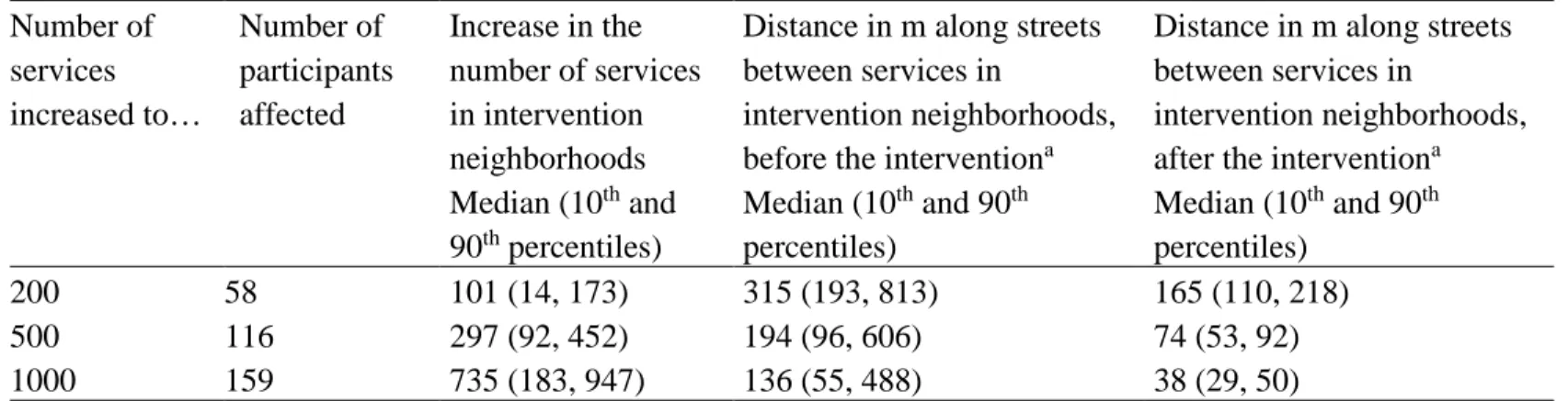
The three hypothetical scenarios of intervention are described in Table 1. For example, the intervention to raise the residential number of services to 200 would affect 58 participants (26%), corresponding to an increase in the number of services by 101 or more in 50% of the cases, and implying a reduction of the distance between services along streets from a median of 315 m to a median of 165 m in the intervention neighborhoods.
Naïve estimates of intervention effects
Based on the regression model reported in eAppendix 4, the probability to walk in a trip
increased with the number of services in the residential neighborhood. As also shown in Figure 4 (panel A), there was a quadratic effect: increases in the number of services beyond 2000 were not associated with further gains in the probability that a trip is walked.
Based on this model, the hypothetical interventions to raise the residential number of services to 200, 500, and 1000 were associated with an increase by 0.020, 0.055, and 0.109 of the
probability that a trip is walked for participants in the intervention groups (Table 2).
Corrected estimates of intervention effects
To derive the corrected intervention effect estimates, we ran the model reported in eAppendix 4 (adjusted for modes used in previous trips and for the trip origin/destination numbers of services). As also shown in Figure 4, the residential number of services was no longer associated with walking (panel B). While the trip origin number of services showed no relationship with walking (panel C), the probability that a trip is walked increased with the number of services around the trip destination (panel D). Again a quadratic effect indicated that the increase in walking
12
associated with an increment of services at the trip destination tended to be lower when the base number of services was high.
Based on the corrected model, the hypothetical interventions to raise the residential number of services to 200, 500, and 1000 led to an increase by 0.007, 0.019, and 0.039 of the probability that a trip is walked for participants in the intervention groups (Table 2). Thus, the naïve estimates overestimated the corrected ones by multiplicative factors of 3.0, 2.9, and 2.8.
DISCUSSION
Contributing to the causal neighborhood effect literature, the present study empirically demonstrates that the “residential” effect fallacy, an overlooked and potentially widespread generator of confounding, was of considerable magnitude for the association between a
residential pseudo-intervention on the number of services and walking. This study estimated an association corrected from the spurious contamination by correlated nonresidential effects.
Strengths and limitations
The primary strength of the present study is that it formally defined a bias, the “residential” effect fallacy, which, despite its general relevance for estimating causal neighborhood health effects, has received no formal consideration in the literature (eAppendix 2 reviews two studies10,33
connected to the present topic but that did not explicitly investigate the bias). Second, this paper could rely on accurate trip-level data obtained through a complex protocol combining GPS tracking, algorithm processing, and related prompted recall survey.8,13,17 The availability of data
disaggregating the behavioral outcome at the level of the multiple places visited by the
participants (in this study the different trips) allowed the empirical identification and correction of the bias, which would have otherwise been impossible. A third strength is our policy-relevant
13
specification of the target causal effect of services that was conceptualized in an interventional perspective (i.e., raising the access to services not by a constant value even in well-served neighborhoods but to a certain level if below that level). However, it should be kept in mind that this pseudo-intervention was not meant to mimic a completely plausible real-world intervention (whose area would not exactly match the precise home-centered buffers of specific individuals) but was seen as an intervention-like formulation of an observational effect estimate, an approach that we recommend for future observational neighborhood studies. As a fourth strength,
eAppendix 5 shows that we were able, not only to quantify the magnitude of the “residential” effect fallacy bias, but also to recalculate the naïve estimate of the residential intervention effect based on an analytical understanding of the mechanism of bias (we could mimic the spurious transfer of nonresidential effects to the “residential characteristic”-walking association attributable to the confounding structure and correlation in the number of services).
Regarding limitations, as detailed in the second section of eAppendix 1, the present work did not consider that an increase in the number of services may also: (i) increase the number of trips and that a similar “residential” effect fallacy may bias this association; and (ii) affect the
destinations and length of trips.
Interpretation of the empirical findings
Our data showed correlation in the local number of services between residential and
nonresidential places over a long range of more than 20 km, supporting the causal structure in Figure 1 and creating a substantial potential for the “residential” effect fallacy.
In the adjusted model that was used to derive a corrected estimate of the residential intervention effect on walking (accounting for the residential, trip origin, and trip destination numbers of services), only the trip destination number of services was associated with walking.
14
This finding that trip destination characteristics are more influential than trip origin
characteristics has already been reported.34 A potential interpretation is that when constraints in
mode choice at the beginning of the trip are taken into account (by controlling for the modes used in previous trips), the environmental conditions at the beginning of the trip loose their predictive importance, and only the spatial accessibility to services at the destination of the trip matters in the adoption or not of walking.
The major finding of our study is that the naïve effect estimates of the residential interventions of interest overestimated the true effects (true effects conditional on a number of assumptions listed in eAppendix 1) by a multiplicative factor of 3. Put the other way round, the correct estimates corresponded to only 35% of the naïve estimates. Clearly, the magnitude of this bias is very substantial compared to biases often documented in studies. The estimated intervention effect on transport walking was relatively modest, especially after applying the correction. Because of this carefully controlled correction and because we could recalculate the naïve intervention effect estimate based on the analytical understanding of the bias (eAppendix 5), we can confidently conclude that the bias of considerable magnitude that was documented was attributable to the “residential” effect fallacy. People travel to various places in their daily
activities35 and the influence of the service environment in these various nonresidential places on
mode choice is spuriously incorporated in the residential effect estimate because of the intra-individual correlation in the exposure to services between residential and nonresidential places.
General implications
The severity of the “residential” effect fallacy, a phenomenon of nonresidential to residential association contamination, depends on the magnitude of confounding and resulting correlation between residential and nonresidential places in the exposure of interest (as influenced to a large
15
extent by the spatial autocorrelation of the exposure over the territory). Because of the urbanization structure of territories and of the socioeconomic distribution of populations, the spatial accessibility to services exhibits a considerable spatial autocorrelation,36 contributing to a
correlation in services between residential and nonresidential neighborhoods visited. For the same reasons and other, many exposures of interest in neighborhood and health studies are likely spatially autocorrelated, such as neighborhood social stressors, fast-food restaurants, alcohol outlets, green spaces, or outdoor noise and air pollution.11,12 Thus a considerable number of
neighborhood or environmental studies exploring associations between residential characteristics and health/behavioral outcomes (cumulating outcome components inside and outside the
neighborhood)1-4 likely yielded substantially overestimated residential effects estimates (although
the bias may be weaker for exposures showing a lower correlation between residential and nonresidential places). Regarding generalization, there is no particular reason why this bias would be of particular importance in France (the marked distinction between urban centers, suburbs, and the countryside and the socioeconomic stratification of territories is widespread across countries).
When studies consider that their residential exposure variable is an imperfect proxy of environmental exposures in the multiple activity places visited, they are not subject to the
“residential” effect fallacy bias described in the present study; however, they are then subject to a severe measurement error because residential exposures are inaccurate proxies of activity space exposures.7,37 As a consequence, classical residential neighborhood studies, depending on the
interpretation of the estimated parameter, are either subject to the “residential” effect fallacy when the association is interpreted as a truly residential effect (due to the similarity between residential and nonresidential neighborhoods) or to measurement error when the association is interpreted as a total environmental effect (due to the dissimilarity between residential and
16
nonresidential neighborhoods, i.e., to the fact that residential neighborhood characteristics are poor proxies of nonresidential characteristics). These two sources of error are likely to be
substantial. Readers are referred to eAppendix 6 for advanced interpretations of the “residential” effect fallacy and sensitivity analyses (e.g., for an estimation of the intervention effect under the assumption that participants are also affected by the intervention in the other participants’ residential areas).
A critical implication of the “residential” effect fallacy is that interventions developed in a residential neighborhood will have a much lower impact on the behavior or health status of residents than would be expected based on the naïve association. In order to reach the impact expected from the estimated association, it would be necessary to intervene, not only in the residential neighborhood but also in various visited locations of the persons (whose impact is spuriously incorporated in the residential effect estimate), which is far more challenging and costly.
For studies without access to individual mobility data, calculation approaches could be
developed to speculate on the magnitude of the “residential” effect fallacy based on knowledge of the spatial distribution of the exposure of interest around participants’ residences and aggregated knowledge of local mobility patterns. However, the recommended strategy is obviously to collect detailed mobility data for each study participant to address both measurement error in
environmental exposures and the “residential” effect fallacy. We suggest to rely on the present design, i.e., to follow participants over time and space, to accurately identify life segments that make up their daily life schedules, to identify momentary exposures in these life segments, and to disaggregate the behavioral outcomes (e.g., physical activity, smoking, alcohol consumption, or food consumption) usually assessed at the individual level at the level of these multiple space-time segments of the days.17 This methodology will allow investigators to disentangle true
17
residential influences from nonresidential effects that otherwise confound the residential
intervention effect estimates of interest. Overall, our key paradox-like message is that to properly investigate residential effects, investigators critically need data on the nonresidential places visited.
18 References
1. Saelens BE, Handy SL. Built environment correlates of walking: a review. Med Sci Sports
Exerc. 2008;40:S550-566.
2. Jackson N, Denny S, Ameratunga S. Social and socio-demographic neighborhood effects on adolescent alcohol use: a systematic review of multi-level studies. Soc Sci Med. 2014;115:10-20.
3. Koohsari MJ, Sugiyama T, Sahlqvist S, Mavoa S, Hadgraft N, Owen N. Neighborhood environmental attributes and adults' sedentary behaviors: Review and research agenda.
Prev Med. 2015;77:141-149.
4. Riva M, Gauvin L, Barnett TA. Toward the next generation of research into small area effects on health: a synthesis of multilevel investigations. J Epidemiol Community Health. 2007;61:853-861.
5. Hernán MA, Hernández-Díaz S, Robins JM. A structural approach to selection bias.
Epidemiology. 2004;15:615-625.
6. Chaix B. Geographic Life Environments and Coronary Heart Disease: A Literature Review, Theoretical Contributions, Methodological Updates, and a Research Agenda.
Annu Rev Public Health. 2009;30:81-105.
7. Chaix B, Kestens Y, Perchoux C, Karusisi N, Merlo J, Meghiref K. An interactive mapping tool to assess individual mobility patterns in neighborhood studies. Am J Prev
Med. 2012;43:440-450.
8. Chaix B, Meline J, Duncan S, et al. GPS tracking in neighborhood and health studies: A step forward for environmental exposure assessment, a step backward for causal
19
9. Kestens Y, Lebel A, Chaix B, et al. Association between activity space exposure to food establishments and individual risk of overweight. PLoS One. 2012;7:e41418.
10. Inagami S, Cohen DA, Finch BK. Non-residential neighborhood exposures suppress neighborhood effects on self-rated health. Soc Sci Med. 2007;65:1779-1791.
11. Shareck M, Kestens Y, Frohlich KL. Moving beyond the residential neighborhood to explore social inequalities in exposure to area-level disadvantage: Results from the Interdisciplinary Study on Inequalities in Smoking. Soc Sci Med. 2014;108:106-114. 12. Krivo LJ, Washington HM, Peterson RD, Browning CR, Calder CA, Kwan MP. Social
Isolation of Disadvantage and Advantage: The Reproduction of Inequality in Urban Space. Soc Forces. 2013;92:141–164.
13. Chaix B, Kestens Y, Duncan S, et al. Active transportation and public transportation use to achieve physical activity recommendations? A combined GPS, accelerometer, and mobility survey study. Int J Behav Nutr Phys Act. 2014;11:124.
14. Brondeel R, Pannier B, Chaix B. Using GPS, GIS, and Accelerometer Data to Predict Transportation Modes. Med Sci Sports Exerc. 2015;47:2669-2675.
15. Sugiyama T, Neuhaus M, Cole R, Giles-Corti B, Owen N. Destination and route attributes associated with adults' walking: a review. Med Sci Sports Exerc. 2012;44:1275-1286. 16. Karusisi N, Thomas F, Meline J, Brondeel R, Chaix B. Environmental conditions around
itineraries to destinations as correlates of walking for transportation among adults: the RECORD cohort study. PLoS One. 2014;9:e88929.
17. Chaix B, Kestens Y, Duncan DT, et al. A GPS-based methodology to analyze environment–health associations at the trip level: case-crossover analyses of built environments and walking. Am J Epidemiol. in press.
20
18. Chaix B, Kestens Y, Bean K, et al. Cohort Profile: Residential and non-residential
environments, individual activity spaces and cardiovascular risk factors and diseases--The RECORD Cohort Study. Int J Epidemiol. 2012;41:1283-1292.
19. Chaix B, Bean K, Daniel M, et al. Associations of supermarket characteristics with weight status and body fat: a multilevel analysis of individuals within supermarkets (RECORD Study). PLoS One. 2012;7:e32908.
20. Chaix B, Bean K, Leal C, et al. Individual/neighborhood social factors and blood pressure in the RECORD Cohort Study: which risk factors explain the associations? Hypertension. 2010;55:769-775.
21. Chaix B, Billaudeau N, Thomas F, et al. Neighborhood effects on health: correcting bias from neighborhood effects on participation. Epidemiology. 2011;22:18-26.
22. Leal C, Bean K, Thomas F, Chaix B. Multicollinearity in the associations between multiple environmental features and body weight and abdominal fat: using matching techniques to assess whether the associations are separable. Am J Epidemiol.
2012;175:1152-1162.
23. Chaix B, Jouven X, Thomas F, et al. Why socially deprived populations have a faster resting heart rate: impact of behaviour, life course anthropometry, and biology - the RECORD Cohort Study. Soc Sci Med. 2011;73:1543-1550.
24. Duncan S, Stewart TI, Oliver M, et al. Portable global positioning system receivers: static validity and environmental conditions. Am J Prev Med. 2013;44:e19-29.
25. Thierry B, Chaix B, Kestens Y. Detecting activity locations from raw GPS data: a novel kernel-based algorithm. Int J Health Geogr. 2013;12:14.
21
26. Frank LD, Saelens BE, Powell KE, Chapman JE. Stepping towards causation: do built environments or neighborhood and travel preferences explain physical activity, driving, and obesity? Soc Sci Med. 2007;65:1898-1914.
27. Brondeel R, Weill A, Thomas F, Chaix B. Use of healthcare services in the residence and workplace neighbourhood: the effect of spatial accessibility to healthcare services. Health
Place. 2014;30:127-133.
28. Chaix B, Simon C, Charreire H, et al. The environmental correlates of overall and neighborhood based recreational walking (a cross-sectional analysis of the RECORD Study). Int J Behav Nutr Phys Act. 2014;11:20.
29. Troped PJ, Wilson JS, Matthews CE, Cromley EK, Melly SJ. The built environment and location-based physical activity. Am J Prev Med. 2010;38:429-438.
30. Cheung YB. A modified least-squares regression approach to the estimation of risk difference. Am J Epidemiol. 2007;166:1337-1344.
31. Austin PC, Laupacis A. A tutorial on methods to estimating clinically and
policy-meaningful measures of treatment effects in prospective observational studies: a review.
Int J Biostat. 2011;7:6.
32. Smith AFM, Roberts GO. Bayesian computation via the Gibbs sampler and related Markov chain Monte Carlo methods. J R Stat Soc Ser B Stat Methodol. 1993;55:3-23. 33. Sharp G, Denney JT, Kimbro RT. Multiple contexts of exposure: Activity spaces,
residential neighborhoods, and self-rated health. Soc Sci Med. 2015;146:204-213. 34. Lee B, Gordon P, Moore JE, Richardson HW. The attributes of residence / workplace
22
35. Perchoux C, Kestens Y, Thomas F, Hulst AV, Thierry B, Chaix B. Assessing patterns of spatial behavior in health studies: Their socio-demographic determinants and associations with transportation modes (the RECORD Cohort Study). Soc Sci Med. 2014;119:64-73. 36. Guillain R, Le Gallo J. Agglomeration and Dispersion of Economic Activities in and
around Paris: An Exploratory Spatial Data Analysis. Environ Plann B. 2010;37:961-981. 37. Zenk SN, Schulz AJ, Matthews SA, et al. Activity space environment and dietary and
23 Figure 1
Directed acyclic graph representing the confounding structure of the “residential” effect fallacy bias with an open backdoor path from the residential exposure to the nonresidential exposure through the macro-organization of the territory. Such macro-organization generates similarity between residential and nonresidential exposures, as modulated however in a complex way by a rich set of determinants of individual mobility. Given the unpredictable way how the macro-organization of the territory and the determinants of individual mobility jointly influence the degree of similarity / dissimilarity between residential and nonresidential exposures, the most straightforward option to close the backdoor path is to directly geocode the nonresidential environments visited and assess related exposures to neutralize confounding.
Figure 2
Illustrative example of two successive trips for a given individual, from the residence (A) to a first visited place (B), and to a second visited place (C). Buffers (1 km street radius) are drawn around each place. The darker buffer represents the residential buffer. For the three successive buffers at visited places, the percentage of overlap with the residential buffer is respectively 100% (A), 30% (B), and 0% (C). The number of services accessible within each 1 km radius buffer was calculated. For the buffer of place B (0 < % overlap < 100) but not for the other buffers, we also calculated the number of services accessible within the portion of the buffer overlapping and not overlapping the residential buffer.
Figure 3
Association between the residential density of services per km² and the trip origin density of services per km² according to the street network distance between the residence and the trip
24
origin (modeled among 3155 trip origins after excluding trips starting at the residence). For example, an increase by 1000 of the residential density of services was associated with an increase by 619 of the number of services per km² around trip origins located 10 km away from the residence (overall Pearson correlation between residential and trip origin densities of services for trip origins located less than 10 km away from the residence = 0.27; 95% confidence interval: 0.23, 0.30).
Figure 4
Increase in the probability that a trip is walked associated with changes in the number of services in the residential neighborhood [naïve estimate model (A) and corrected estimate model (B)], with the trip origin number of services [corrected estimate model (C)], and with the trip destination number of services [corrected estimate model (D)] (number of services = 0 as the reference).
Macro-organization
of territory:
- rural vs urban
- socioeconomic
Low/high residential
neighborhood
exposure
Comparably
low/high exposure in
visited places
Intervention
Health or behavioral
outcome
Determinants
of individual
mobility
Macro-organization
of territory:
- rural vs urban
- socioeconomic
Low/high residential
neighborhood
exposure
Comparably
low/high exposure in
visited places
Intervention
Health or behavioral
outcome
1 Figure 2
1 Figure 4
Table 1. Description of the hypothetical scenarios of intervention on the number of services in the residential neighborhood Number of services increased to… Number of participants affected Increase in the number of services in intervention neighborhoods Median (10th and 90th percentiles)
Distance in m along streets between services in
intervention neighborhoods, before the interventiona
Median (10th and 90th
percentiles)
Distance in m along streets between services in
intervention neighborhoods, after the interventiona
Median (10th and 90th
percentiles)
200 58 101 (14, 173) 315 (193, 813) 165 (110, 218)
500 116 297 (92, 452) 194 (96, 606) 74 (53, 92)
1000 159 735 (183, 947) 136 (55, 488) 38 (29, 50)
aThe calculation of distance between services along streets combines services on both sides of the street (a service
on the left side followed by another service 20 m after on the right side of the road correspond to a distance of 20 m between services). Dual carriageways, however, intervene as two separate streets in the calculation. Non walkable highways and speedways are not accounted for in this calculation.
1
Table 2. Naïve and corrected estimates of the hypothetical intervention effect of raising the number of services in
the residential neighborhood to 200, 500, or 1000 for participants in the intervention groups (i.e., with a residential number of services below 200, 500, or 1000)a
Intervention: residential number of services raised to 200
Intervention: residential number of services raised to 500
Intervention: residential number of services raised to 1000
Naïve estimate 0.020 (0.010, 0.029) 0.055 (0.030, 0.079) 0.109 (0.063, 0.154) Corrected estimate 0.007 (0.001, 0.014) 0.019 (0.000, 0.038) 0.039 (0.004, 0.073)
aThe exact sets of predictors included in the naïve estimate model and in the corrected estimate model are reported
1
eAppendix
The “residential” effect fallacy in neighborhood and health studies: formal definition, empirical identification, and correction
EAPPENDIX 1: ASSUMPTIONS REQUIRED FOR ESTIMATING A VALID CAUSAL RESIDENTIAL
INTERVENTION EFFECT 2
1)ESTIMATION OF THE REGRESSION MODEL USED FOR THE CALCULATION 2
2)CALCULATION OF THE RESIDENTIAL INTERVENTION EFFECT ESTIMATE BASED ON THE REGRESSION ESTIMATES 4
EAPPENDIX 2: REVIEW OF PREVIOUS LITERATURE 7
INAGAMI ET AL. 7
SHARP ET AL. 8
EAPPENDIX 3: SERVICES ACCOUNTED FOR IN OUR SPATIAL ACCESSIBILITY VARIABLE 10 EAPPENDIX 4: REGRESSION MODELS ESTIMATED TO DETERMINE THE NAÏVE AND CORRECTED
INTERVENTION EFFECT ESTIMATES 13
EAPPENDIX 5: A POSTERIORI RECALCULATION OF THE NAÏVE BIASED RESIDENTIAL INTERVENTION
EFFECT ESTIMATE 14
METHODOLOGY 14
RESULTS 15
EAPPENDIX 6: ADVANCED INTERPRETATION OF THE “RESIDENTIAL” EFFECT FALLACY BIAS 19
SOURCE OF THE CORRELATION BETWEEN EXPOSURES AT THE RESIDENTIAL AND NONRESIDENTIAL PLACES VISITED 19
OVERALL BEHAVIORAL OUTCOME VS. RESIDENTIAL NEIGHBORHOOD-SPECIFIC BEHAVIORAL OUTCOME 19
CAN THE “RESIDENTIAL” EFFECT FALLACY LEAD TO AN UNDERESTIMATION OF RESIDENTIAL EFFECTS? 20
INTERFERENCES BETWEEN PARTICIPANTS 20
2
eAppendix 1: Assumptions required for estimating a valid causal residential intervention effect
In this paper, we aimed to estimate the causal effect of a hypothetical intervention raising the residential number of services on the probability that a trip is walked. There are potential concerns about drawing causal inferences based on our estimate, even after the correction of the “residential” effect fallacy. Below, we provide a tentative list of assumptions that would need to be met so that the estimate of the residential intervention effect corrected from the “residential” effect fallacy represents the causal intervention effect.
1) Estimation of the regression model used for the calculation
• We assume no systematic measurement error in the probability that a trip is walked according to the exposure variable (the residential accessibility to services).
• We assume no systematic measurement error in the number of services across the different types of transport modes (e.g., differential misclassification of the count of services according to the type of place, itself associated with a particular mode use). • We assume no systematic nondifferential measurement error in the number of services
(i.e., a uniform decrease or increase in the count of services), which would bias the intervention effect estimate due to the nonlinear relationship between the number of services and walking.
• Also we make the assumption of no random measurement error in the number of services (i.e., the exposure) which, as a regression dilution bias, would result in an attenuation towards the null of the association between the exposure to services and the probability that a trip is walked.
• We assume no random measurement error in the transport outcome, which would increase the standard error of the estimated association.
3
• The study examined the association between the number of services in a 1 km radius buffer around the residence and walking. This was not considered to be an assumption of the study (that would be related to the expected spatial scale of this causal
determinant of walking), but to be a logical consequence of the hypothetical choice of policymakers to intervene within 1 km of the residence of a number of residents. However, when we attempted to estimate the causal effect of the number of services around the trip origins and destinations, we also chose a 1 km radius for the trip
origin/destination buffers for the sake of coherence. This was related to the assumption that the causal effect that we attempted to take into account (as a potential confounder of the intervention effect) was best captured with a radius of 1 km. It might be that the optimal radius to capture this effect is shorter. However, this is likely not of critical importance due to the strong autocorrelation in the number of services that should minimize the impact of small differences in the radius to define the buffers. • We assume that there is no selection bias in the sample used for estimating the
association of interest. Specifically, we assume that the participation in the sample is not influenced by both the exposure (or a determinant of the exposure) and the outcome (or a determinant of the outcome).
• We assume that there is no additional unmeasured trip-level, individual-level, or environmental confounders in the relationship between the residential number of services and the probability of walking, after our correction of the “residential” effect fallacy and after accounting for neighborhood preferences at the time of moving in one’s current neighborhood (neighborhood selection factors) and the other covariates. We assume that residents of neighborhoods with different levels of spatial
4
• We assume that the positivity assumption (or experimental treatment assignment assumption) is held. We assume that there are both exposed and unexposed individuals at every combination of levels of the observed confounders in the population of
interest. Under this assumption, our regression modeling is not based on excessive extrapolations.
• The random effect linear probability model including linear and quadratic terms for the service accessibility variables is assumed to be not misspecified. The following standard assumptions are hypothesized to apply: homoscedasticity; normal distribution of residuals at the trip level and at the individual level; and absence of correlation between the exposure of interest or other covariates and the level-2 individual-level random intercept.
2) Calculation of the residential intervention effect estimate based on the regression estimates
• The method acknowledges that the residential intervention may also influence mode choice in trips far from the residence through the influence that the residential neighborhood has on the overall choice of mode (e.g., buying a car or a public
transport pass). This is not an assumption that we force into the model, but a potential mechanism that is allowed for in the model and that is incorporated into the
calculation only if estimated to be at play.
• We assume that there is no relevant time varying environmental variable correlated with the implementation of the intervention of interest. For example, if interventions aiming at increasing the number of services were systematically implemented simultaneously with urban design changes (i.e., if the two were consubstantial), the true, pure intervention effect would not correspond to the one estimated in this study. • Provided that the assumptions listed above are satisfied, the regression estimates
5
and trip origin neighborhoods on walking. However, these causal effects are averages of heterogeneous effects across different population subgroups. Our calculation assumes that the various neighborhoods in our study territory contain a comparable mix of heterogeneous residents leading to a uniform intervention effect on walking. • We make the assumption that the intervention (increase in the number of services) is
evenly distributed over the 1 km residential buffer; thus the portion of the residential intervention that affects a participant located in a nonresidential place depends on the fraction of the residential buffer that is included in this nonresidential buffer.
• The calculation of the residential intervention effect estimate was based, among other, on the estimated associations between the trip origin/trip destination numbers of services and walking. These were average effects, i.e., the associations between the trip origin or trip destination number of services and walking were estimated
accounting for all trip origins and destinations in the database. However, this estimate was used to calculate the intervention effect estimate for trip origins and destinations close to the residence (as their buffer had to overlap the residential buffer). Thus we hypothesize that the estimated associations between the trip origin/destination numbers of services and walking were appropriate to estimate the intervention effect for trip origins/destinations overlapping the residential buffer.
• In the calculation of the overall intervention effect estimate based on the regression estimates, an absence of residential migration between the pre-intervention and post-intervention states is assumed. Also, we assume no change in the places visited for this calculation. Regarding the notion of post-intervention disequilibria, our calculation is based on the stable unit treatment assumption, i.e., the intervention implemented for one person does not affect the level of intervention for another person. While this assumption was made in the calculations in the main article, the last section of
6
eAppendix 7 provides calculations relaxing this assumption of an absence of interferences between participants.
• It should be noted that the present work took into account the “residential” effect fallacy only in the association of services with the probability that a trip is walked. However, our calculations did not account for the fact that an increase in the
residential number of services may also increase the number of trips, and that a similar “residential” effect fallacy may bias this association. Correcting for the “residential” effect fallacy in the number of trips would be more complicated.
• Moreover, an intervention on services in the residential neighborhood may affect not only the number of trips but also the length of trips and how trip origins / destinations are close or not from the residence.1 Because our regression models were purposely
not adjusted for distance, the association estimated between services and walking may operate through a switch of mode in a given trip with fixed start and end points but also through a switch from a longer motorized trip to a shorter walking trip. However, our estimation of the intervention effect did not allow for a change in the extent to which the origin and destination buffers of each trip overlapped the residential
neighborhood. This is a limitation since an intervention raising the residential number of services may increase the percentage of trips whose origin and/or destination buffers overlap the residential neighborhood. Thus our illustrative study was to some extent grounded on the simplifying hypothesis that participants would anyway visit all the places visited during the follow-up even if the residential number of services was increased.
7 eAppendix 2: Review of previous literature
There are very few articles in the whole literature on neighborhood / environmental effects on health that relate at least approximately to the topic of the “residential” effect fallacy bias that we describe.
Inagami et al.
In a well-known article,2 Inagami and colleagues found that a low socioeconomic status of the
residential neighborhood was associated with a worst self-rated health; that exposure to a low socioeconomic status in nonresidential neighborhoods was associated with a worst self-rated health (only in some of the models); and that adding the nonresidential term to the model increased the residential effect estimate. Thus the standard calculation of the residential effect estimate led to an underestimation of the supposedly true residential effect, i.e., the
confounding bias was in the form of a suppression effect rather than an amplification effect as in our article.
However, the conceptual and analytical framework of Inagami and colleagues was entirely different from ours. In the work of Inagami, the nonresidential exposure variable was
calculated as the difference between the nonresidential exposure and the residential exposure, thus expressed as nonresidential relative disadvantage. First, it should be noted that such a “relative exposure effect” is an original effect in itself, distinct from the effect of the absolute level of nonresidential exposure we are interested in. Indeed, such a relative exposure
specification likely captures a different effect operating through distinct mechanisms, such as the influence of cognitive processes of comparison of residential and nonresidential
neighborhoods. Second, Inagami and colleagues implicitly recognize that there was a positive correlation between the absolute socioeconomic status in the residential and nonresidential
8
neighborhoods (Data and methods, Measures, Operationalizing non-residential neighborhood exposure, fourth paragraph). However, the suppression effect of confounding documented by Inagami (rather than amplification effect in our case) implies a negative correlation between the residential socioeconomic status and nonresidential socioeconomic exposure variable (as opposed to a positive correlation in our “residential” effect fallacy application). This negative correlation stems from the relative definition of the nonresidential exposure that was used (difference with the residential exposure) and may be attributable to a “regression to the mean”, i.e., to the fact that participants with a particularly high residential socioeconomic status will often have nonresidential places with a comparably lower socioeconomic status (thus a negative relative exposure) while participants with a particularly low residential socioeconomic status will often have nonresidential places with a comparably higher socioeconomic status.
Overall, the study by Inagami and colleagues investigates how a nonresidential effect defined in a different way than the residential effect (relative exposure) negatively confounds the residential effect of interest. Differently, our study investigates how a nonresidential effect defined in a similar way than the residential effect positively confounds the residential effect. Thus our study is the first to address the “residential” effect fallacy bias described here.
Sharp et al.
Another article by Sharp and colleagues3 based on longitudinal data from the same cohort
than in the Inagami article examined the extent to which controlling for the exposure to nonresidential neighborhood disadvantage affected the relationship between residential neighborhood disadvantage and self-rated health. As opposed to Inagami et al., nonresidential disadvantage was assessed in absolute rather than relative terms. The work by Sharp and colleagues reported that the residential effect estimate was slightly attenuated when the model
9
was adjusted for nonresidential exposures. This reduction of the strength of the association was attributed to a mediation of the residential association by the nonresidential term, although no concrete description of the causal mechanism involved in this supposed mediation and no explanation based on directed acyclic graphs of why this should be mediation rather than confounding were provided. Even if the observed reduction in the residential association when controlling for the nonresidential term is coherent with our own findings, the conceptual framework that we develop is substantially different. Although we acknowledge that nonresidential exposures mediate to some extent the estimated residential neighborhood-walking association (the residential environment influences the transport modes used, which influence the types of places visited), we emphasize that most importantly, nonresidential exposures confound the residential neighborhood-walking association.
10
eAppendix 3: Services accounted for in our spatial accessibility variable
Consistent with previous literature,4-6 the spatial accessibility to destinations within a walking
distance has been found to be a major determinant of both transport and recreational walking in our RECORD Study.7-9 Services, especially because a large spectrum of them were
accounted for in our study, represent a large share of the potential destinations of participants. Thus, our variable is expected to capture in a relatively reliable way a factor that has a direct causal effect on the likelihood of transport walking.
We report below the list of services accounted for in our variable of spatial accessibility to services. Although neither sport facilities nor parks were taken into account in the list of services that was analyzed, it can be seen that a large fraction of the services available were included in this study.
List of services analyzed: A101 – Police
A102 – Treasury
A103 – National Employment Agency A104 – Gendarmerie
A203 – Bank A206 – Post office
A207 – Package delivery point A208 – Municipality post office A301 – Car repair
A302 – Automobile technical inspection service A303 – Car rental
A401 – Mason
A402 – Plasterer, painter
A403 – Wood worker, carpenter, locksmith A404 – Plumber, roofer, heating engineer A405 – Electrician
A406 – Construction company A501 – Hairdresser
A502 – Veterinarian A504 – Restaurant
A505 – Real estate agency A506 – Laundry
11 B101 – Hypermarket
B102 – Supermarket
B103 – Large do-it-yourself store B201 – Minimarket
B202 – Grocery B203 – Bakery
B204 – Butcher / delicatessen shop B205 – Frozen food store
B206 – Fish market
B301 – Bookshop, stationery store B302 – Clothing store
B303 – Home equipment store B304 – Shoe store
B305 – Home appliance store B306 – Furniture store B307 – Sports store
B308 – Wallpaper and wall covering store B309 – Drugstore, hardware, handiwork B310 – Perfumery
B311 – Watch and jewellery B312 – Florist
B313 – Optical store D108 – Health center
D201 – General practitioner D202 – Cardiologist
D203 – Dermatology and venereology D204 – Medical gynecology D205 – Gynecology obstetrics D206 – Gastroenterology D207 – Psychiatry D208 – Ophthalmology D209 – Otorhinolaryngology D210 – Pediatrics D211 – Pulmonology
D212 – Diagnostic radiology and medical imaging D213 – Stomatology D221 – Dental surgeon D231 – Midwife D232 – Nurse D233 – Masseur physiotherapist D235 – Speech therapist D236 – Orthoptist D237 – Chiropodist D238 – Audioprosthesist D239 – Occupational therapist D240 – Psychomotrician
D241 – Medical radiology operator D301 – Pharmacy
D302 – Medical analysis laboratory F301 – Cinema
12 F302 – Theater
13
eAppendix 4: Regression models estimated to determine the naïve and corrected intervention effect estimates
eAppendix Table 1. Regression models estimated to determine the naïve and corrected residential intervention
effect estimates
Model for the naïve estimate
Model for the corrected estimate Individual factors Age (vs. 35–49) 50–64 +0.02 –0.08, +0.12 +0.02 –0.06, +0.09 65 and over –0.02 –0.16, +0.13 –0.02 –0.12, +0.09 Male (vs. female) –0.03 –0.11, +0.05 –0.02 –0.08, +0.04
Living alone (vs. as a couple) –0.02 –0.11, +0.07 –0.05 –0.11, +0.02
Education (vs. ≤ low secondary)
Upper secondary, low tertiary –0.02 –0.12, +0.07 –0.02 –0.09, +0.05
Intermediate tertiary +0.09 –0.03, +0.21 +0.04 –0.05, +0.12
Upper tertiary –0.07 –0.17, +0.03 –0.06 –0.13, +0.02
Employment status (vs. stable job)
Precarious job –0.07 –0.27, +0.14 –0.02 –0.18, +0.13
Unemployment +0.16 –0.09, +0.41 +0.14 –0.04, +0.33
Household income per consumption unit (vs. ≤1285 €)
>1285 – ≤2200 € +0.00 –0.08, +0.09 +0.01 –0.06, +0.08
>2200 € –0.02 –0.11, +0.08 +0.00 –0.07, +0.07
Services as a neighborhood selection factor (vs. low)
Intermediate +0.05 –0.07, +0.15 +0.06 –0.02, +0.14
High +0.05 –0.06, +0.16 +0.06 –0.03, +0.14
Public transport as a neighborhood selection factor (vs. low)
Intermediate –0.03 –0.15, +0.10 –0.01 –0.10, +0.08
High –0.01, –0.11, +0.09 –0.02 –0.10, +0.06
Bike used in previous trips from home – –0.51 –0.59, –0.44
Personal vehicle used in previous trips from home (vs. no)
In some of the trips – –0.32 –0.37, –0.27
In all trips – –0.56 –0.60, –0.53
Environmental factors
Number of services, residential neighborhood
Linear term +0.21 +0.11, +0.32 +0.02 –0.07, +0.10
Quadratic term –0.04 –0.07, –0.01 –0.01 –0.03, +0.02
Number of services, trip origin
Linear term – +0.03 –0.02, +0.08
Quadratic term – –0.01 –0.02, +0.00
Number of services, trip destination
Linear term – +0.10 +0.05, +0.15
14
eAppendix 5: A posteriori recalculation of the naïve biased residential intervention effect estimate
Methodology
To reach an analytical understanding of the genesis of the bias, we recalculated the naïve estimate of the intervention effect from a model accounting for the trip-level number of services. In our naïve model, influences on walking of the nonresidential places visited are spuriously incorporated in the residential neighborhood-walking association when the number of services at these visited places is similar to the residential number of services. Our aim was to mimic this process.
To do so, we had to determine whether the number of services in each nonresidential place visited was “similar” or not to the residential number of services. For the nonresidential place of a participant X, we constructed a database comprising this nonresidential place of X and all the nonresidential places of the other participants. For each of these nonresidential places in the database, we calculated the absolute value of the difference between the nonresidential number of services and the residential number of services of participant X. The number of services in the participant X’s nonresidential place buffer was considered to be similar to participant X’s residential number of services if the corresponding difference was below the first decile, the second decile, the third decile, the fourth decile, or the fifth decile of ranked differences (alternative definitions of “similarity”).
In our recalculation of the naïve estimate, the number of services in a nonresidential place (even if not overlapping the residential neighborhood) was spuriously raised to the
intervention target (200, 500, or 1000) if this nonresidential place was “similar” to the residential neighborhood in terms of services.
15
To recalculate the naïve intervention effect estimate, we re-estimated the regression model for walking with sociodemographic variables, neighborhood selection factors, and the residential, trip origin, and trip destination numbers of services as explanatory variables but without modes used in previous trips (as nonresidential effects incorporated in the naïve estimate are confounded by these modes in previous trips). Based on model coefficients, we calculated the predicted probability of entirely walking in each trip from all model covariates (including the residential, trip origin, and trip destination numbers of services, modified as explained above). This calculation was performed for the pre-intervention state and for each of the post-intervention scenarios (residential services raised to 200, 500, or 1000). For each of these four cases, we calculated the average probability of walking in a trip across all individuals and trips. The intervention effect estimate was computed for each intervention level, and for each cutoff to define whether a nonresidential place was similar to the
residential neighborhood in terms of services, as the post-intervention average probability of walking minus the pre-intervention probability, only among participants who experimented the hypothetical intervention (i.e., with less than 200, 500, or 1000 services in their residential neighborhood).
Results
The model that was estimated is reported in eAppendix Table 2. When no adjustment was made for the modes in previous trips, both the trip origin and trip destination numbers of services were positively associated with the probability that a trip is walked (with quadratic effects).
The recalculation of the naïve biased estimate implied to spuriously integrate in the residential neighborhood-walking association the influence on walking of the nonresidential places visited if their number of services was “similar” to the residential number of services.